HAL Id: hal-02416248
https://hal.archives-ouvertes.fr/hal-02416248
Submitted on 17 Dec 2019
HAL is a multi-disciplinary open access
archive for the deposit and dissemination of sci-entific research documents, whether they are pub-lished or not. The documents may come from teaching and research institutions in France or abroad, or from public or private research centers.
L’archive ouverte pluridisciplinaire HAL, est destinée au dépôt et à la diffusion de documents scientifiques de niveau recherche, publiés ou non, émanant des établissements d’enseignement et de recherche français ou étrangers, des laboratoires publics ou privés.
OECD-WGAMA CFD activities
D. Bestion
To cite this version:
D. Bestion. BEPU methods using CFD codes -Progress made within OECD-WGAMA CFD activities. ANS Best Estimate Plus Uncertainty International Conference (BEPU 2018), May 2018, Lucca, Italy. �hal-02416248�
BEPU METHODS USING CFD CODES -
PROGRESS MADE WITHIN OECD-WGAMA CFD ACTIVITIES
D. Bestion
Commissariat à l’Energie Atomique CEA-GRENOBLE, DEN-DM2S-STMF, 17 Rue des Martyrs, GRENOBLE Cedex, FRANCE
Dominique.bestion@cea.fr
ABSTRACT
Best-estimate plus uncertainty (BEPU) methods are now commonly used in licensing with system thermalhydraulic codes. It required three decades of efforts to develop best-estimate (BE) codes, and to verify and validate them, to reduce the “User Effect” and to develop methods for code uncertainty quantification. This paper summarizes more recent efforts made to extend BEPU methods to the application of CFD for safety analyses. OECD-NEA-CSNI Working Group for Analysis and Management of Accidents (WGAMA) initiated activities in 2003 in order to promote the use of CFD for nuclear safety. “Best Practice Guidelines (BPG) for Use of CFD on Nuclear Reactor Safety Application” were established. A document was written on the “Assessment of CFD Codes for Nuclear Reactor Safety Problems” with a compendium of current application areas and a catalogue of experimental validation data relevant to these applications. The “Extension of CFD Codes to Two-Phase Flow Safety Problems” was also treated in a separate document, including some first Best Practice Guidelines for two-phase CFD application to some selected NRS problems. Then a review of uncertainty methods for CFD applications was written. International benchmarks were also organized to test CFD capabilities to address reactor issues such as thermal fatigue, flow in a rod bundle with specific influence of spacer grids, hydrogen mixing in a containment. The last benchmark was the first Uncertainty Quantification exercise on a rather simple mixing problem in presence of buoyancy effects. This paper summarizes the main outcome of these 15 years activities with particular attention to uncertainty methods and results of the last benchmark. Both uncertainty propagations methods and accuracy extrapolation methods were used with some success to the GEMIX benchmark. The degree of maturity of all the methods is still rather low but results obtained so far are encouraging. The paper will conclude on a detailed state of the art of BEPU methodologies applied with CFD simulations with an identification of the main difficulties and limitations of current approaches. Further activities are recommended to go beyond the present limitations and on-going WGAMA activities are mentioned.
1. INTRODUCTION
Best-estimate plus uncertainty (BEPU) methods are now commonly used in licensing with system thermalhydraulic codes. It required three decades of efforts to develop best-estimate (BE) codes,
and to validate them on a very large data base of separate-effect tests (SETs) and integral-effect tests (IETs). It also required long efforts to reduce the “User Effect” by defining precise User’s Guidelines”, by developing the expertise among code users. At last, methods for code uncertainty quantification were developed, tested, benchmarked and finally are now being used for safety demonstration.
Among safety investigations, some accident sequences involve complex 3D phenomena in complex geometries which cannot be well described by system codes, and CFD codes started being used to solve them. Before being acceptable for licensing, similar requirements as for system codes have to be met and OECD-NEA-CSNI Working Group for Analysis and Management of Accidents (WGAMA) initiated activities in 2003 in order to promote the use of CFD for nuclear reactor safety (NRS). Three separate Writing Groups (WG) were created.
WG1 established the “Best Practice Guidelines” (BPG) for the Use of CFD in Nuclear Reactor Safety Applications” (Mahaffy, 2007[1], 2015 [2]) with a set of guidelines for a range of single phase applications of CFD. A Process Identification and Ranking Table (PIRT) provides the basis for selection of an appropriate simulation tool, and establishes the foundation for the validation process needed for confidence in final results. Guidance is first given in the selection of physical models available as user options including Reynolds Averaged Navier Stokes (RANS), Large Eddy Simulation (LES), and hybrid approaches. Guidelines are provided for nodalization and for selecting numerical options. The general assessment strategy is discussed with Validation and Verification. Examples of nuclear reactor safety (NRS) applications are considered such as boron dilution and pressurized thermal shock. This first activity was necessary to avoid too much User Effect since existing CFD tools offer many numerical and physical options, and the quality of the nodalization plays a major role.
WG2 produced a document on the “Assessment of CFD Codes for Nuclear Reactor Safety Problems” (Smith et al, 2008 [3], 2015 [4]) with a compendium of current application areas and a catalogue of experimental validation data relevant to these applications. Gaps in information are identified, and recommendations on what to do about them are made with a focus on single-phase flow situations. A list of NRS problems for which CFD analysis is expected to bring real benefits has been compiled, and reviewed critically. Validation data from all available sources has been assembled and documented. Assessment databases relating to specific NRS issues has been catalogued separately, and more comprehensively discussed. Areas here include boron dilution, flow in complex geometries, pressurized thermal shock and thermal fatigue. Gaps in the existing assessment databases are identified.
WG3 treated the “Extension of CFD Codes Application to Two-Phase Flow Safety Problems” (Bestion et al, 2006, [5], 2010 [6], 2014 [7], Bestion, 2010 [8]). A report listed 25 NRS problems where two-phase CFD may bring real benefit, classified different modelling approaches, specified and analyzed needs in terms of physical and numerical assessment. Each issue has been ranked with respect to the degree of maturity of present tools for solving them. Gaps in modelling approaches have been identified with particular attention to the filtering of equations, to the dispersed flows and the free surface flows. A first list of numerical benchmarks was collected. The foundation of Best Practice Guidelines for two-phase CFD application to the selected NRS problems was added.
Later a review of uncertainty methods applied to CFD application to NRS was made showing a rather low degree of maturity of existing methods (Bestion et al., 2016 [9], Bestion & Moretti., 2016 [10]).
International benchmarks were also organized to test CFD capabilities to address reactor issues. A first benchmark was based on a mixing Tee experiment for investigating thermal fatigue. The second benchmark addressed flow in a rod bundle with specific influence of spacer grids. The third benchmark addressed physical processes (particularly stratification erosion) occurring in a containment following a postulated severe accident in which there is a significant build-up of hydrogen in the containment atmosphere. The last benchmark was the first Uncertainty Quantification (UQ) exercise on a rather simple mixing problem in presence of buoyancy effects. This paper summarizes the progress made in the past 15 years in the application of CFD to NRS, starting with PIRT and scaling analyses, code option selections, V&V, and later UQ methods. The results of the four benchmarks are summarized to identify the remaining needs to improve the reliability and maturity of CFD application within BEPU methods.
2. THE DOMAIN OF POSSIBLE APPLICATION OF BEPU METHODS WITH CFD
NRS applications where CFD may bring a real benefit were listed in WG2 report [3,4] which focussed on single-phase issues; two-phase phenomena were also listed for completeness, but full details were reserved for the WG3 report [5,6,7] document which addresses the extensions necessary for CFD to handle such problems.
Considering only single phase issues most of them are related to turbulent mixing problems, including temperature mixing or mixing of chemical components in a multi-component mixture (boron in water, Hydrogen in air,…) with possible effects of density gradients and natural circulation:
Boron dilution
Steam line break (MSLB) with mixing in the Pressure Vessel (PV) between cold water coming from the broken loop and hotter water coming from the others
Pressurised thermal shock (PTS)
Mixing: stratification and hot-leg temperature heterogeneities Thermal fatigue
Erosion, corrosion and deposition
Heterogeneous flow distribution (e.g. in SG inlet plenum causing vibrations,., etc.) BWR/ABWR lower plenum flow
Induced break
Hydrogen distribution in containment Chemical reactions/combustion/detonation
Special considerations for advanced (including Gas-Cooled) reactors
All these mixing problems may be simulated with both Reynolds Average Navier Stokes (RANS) and Large Eddy Simulation (LES) models of turbulence, but RANS models require less CPU cost and are still likely to be preferred. The choice between the various types of turbulence models may depend on the situations and some Guidelines are given in the report of the Writing Group 1 ([1,2]).
Among the mixing problems listed here above only the thermal fatigue requires that low frequency fluctuations be predicted which almost excludes RANS approaches and gives a strong added value to the Large Eddy Simulation (LES).
WG3 identified a list of 25 NRS problems for which two-phase CFD may bring real benefit [5,6,7]. Each issue was examined and classified with respect to the degree of maturity of present CFD tools to resolve it in the short or medium term. Some NRS problems require two-phase CFD in an open medium, and others in a porous medium approach. For some problems, investigations with a two-phase CFD tool for an open medium were used for a better understanding of the flow phenomena, and for developing appropriate closure relations for a 3-D model of the porous medium type. Among these issues one may find the following objectives of CFD investigation:
Issues with 3D flow in large scale open medium such as a containment, pool heat exchangers, external pressure vessel cooling,…
Issues for which a fine space or time resolution is needed such as PTS, thermal fatigue, erosion and corrosion,…
Issues which are revisited with a local analysis for a better understanding of the physics and a more accurate and reliable prediction, such as
o Boiling bubbly flow for Departure from Nucleate Boiling (DNB) investigations o Annular-mist flow for Dry-Out investigations
o Core reflooding in design basis (DBA) and beyond design basis accidents (BDBA) Issues with flow dependent on small scale geometrical effects:
o DNB, Dry-out with spacer grid effects o DBA reflooding with spacer grid effects o BDBA Reflooding of debris bed
o Erosion corrosion at steam generator (SG) support plates o 2 Phase flow in valves
o Pressure losses, cavitation, choked flow in singular geometries o Components with complex geometry (separators, dryers,..) o 2-phase flow in pumps
Significant progress was obtained in the past 15 years particularly in boiling flow simulations, 2-phase PTS scenarios, cavitation, reflooding, containment 2-2-phase issues,
3. THE VARIOUS STEPS OF A BEPU APPROACH
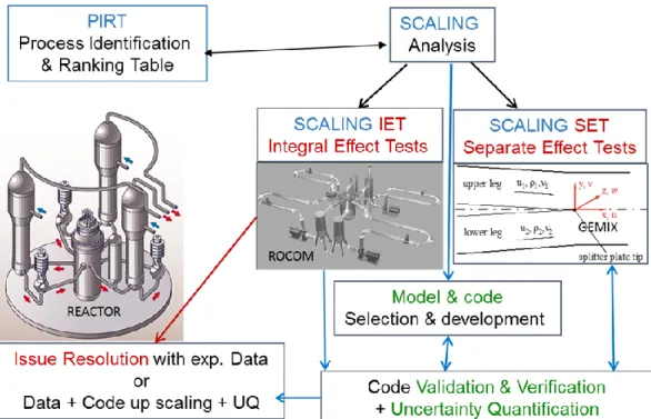
The reactor safety demonstration requires the analysis of complex problems related to accident scenarios. The experiments cannot reproduce at a reasonable cost the physical situation without any simplification or distortion, and the numerical tools cannot simulate the problem by solving the exact equations. Only reduced scale experiments are feasible to investigate the phenomena and only approximate systems of equations may be solved to predict time and/or space averaged parameters with errors due to imperfections of the closure laws and to numerical errors. Therefore complex methodologies are necessary to solve a problem including a PIRT analysis, a scaling analysis, the selection of scaled Integral Effect Tests (IET) or Combined effect tests (CET) and Separate Effect Tests, the selection of a numerical simulation tool, the Verification and Validation of the tool, the code application to the safety issue of interest and the use of an uncertainty method to determine the uncertainty of code prediction. This global approach is illustrated in Figure 1.
Figure 1 – BEPU Methodology for Solving a Reactor Thermalhydraulic Issue.
The PIRT
Phenomena identification is the process of analyzing and subdividing a complex system thermal-hydraulic scenario (depending upon a large number of thermal-thermal-hydraulic quantities) into several simpler processes or phenomena that depend mainly upon a limited number of thermal-hydraulic quantities.
During the physical analysis, it is useful to discern the dominant parameters (figures of Merit - FoM) with the parameters which have an influence on it (FoM). For CFD studies, FoMs are those which play a key role directly on the safety criterion. Depending on the safety scenario, the FoM can be a scalar or a multidimensional value (over space and/or time) or a dimensionless number. For any type of FoM, the required accuracy must be specified and must be kept in mind when judging the pertinence of all later steps of the VVUQ process;
Ranking means here the process of establishing a hierarchy between identified processes with regards to their influence on the figures of Merit.
PIRT is a formal method described in Wilson & Boyack (1998, [11]). Its use is recommended by OCDE WGAMA BPG [1,2]. The main steps of the physical analysis based on PIRT are:
Establish the purpose of the analysis and specify the reactor transient (or situation) of interest
Define the dominant parameters or FoM (figures of Merit) List the involved physical phenomena and associated parameters
Identify and rank key phenomena (or the parameters associated to each phenomenon) with respect to their influence on the FoM.
Identify dimensionless numbers controlling the dominant phenomena
PIRT can be based on expert assessment, on analysis of some experiments, and on sensitivity studies using simulation tools. Practically, PIRT analysis traditionally relied more heavily on the first one, while WGAMA recommendation is to perform sensitivity analysis to get a better
justification in a NRS demonstration (PIRT Validation). NRC Regulatory Guide 1.2.0.3 mentioned exactly the same position for the EMDAP (Evaluation method for codes), as following:
"The initial phases of the PIRT process described in this step can rely heavily on expert opinion,
which can be subjective. Therefore, it is important to validate the PIRT using experimentation and analysis……Sensitivity studies can help determine the relative influence of phenomena identified early in the PIRT development and for final validation of the PIRT as the EMDAP is iterated."
One can start with expert assessment and then iterate with sensitivity studies to refine the PIRT conclusions.
More precisely the PIRT applied to an issue where CFD may be the selected simulation tool may include the following steps:
Problem definition and PIRT objective
Clear definition of the reactor transient of interest and simulation domain
Identification of the dominant physical phenomena including typical 3D thermalhydraulic phenomena that CFD can describe,
Discern the FoM and the parameters which have an influence on FoM Definition of the quantity of interest,
Dimensionless numbers describing the dominant physical phenomena.
Scaling
The word scaling can be used in a number of contexts: two of these may be concerned hereafter: 1. Scaling of an experiment is the process of demonstrating how and to what extent the
simulation of a physical process (e.g. a reactor transient) by an experiment at a reduced scale (or at different values of some flow parameters such as pressure and fluid properties) can be sufficiently representative of the real process in a reactor.
2. Scaling applied to a numerical simulation tool is the process of demonstrating how and to what extent the numerical simulation tool validated on one or several reduced scale experiments (or at different values of some flow parameters such as pressure and fluid properties) can be applied with sufficient confidence to the real process.
When solving a reactor thermalhydraulic issue the answer to the issue may be purely experimental but usually both experiments and simulation tools are necessary. This means that the simulation tool is used to extrapolate from experiments to reactor situation - this is the upscaling process- and the degree of confidence on this extrapolation is part of the scaling issue.
The extrapolation to a reactor situation requires an extrapolation method of the FoM to different values of the Re number and any other non-dimensional numbers at reactor scale, and an extrapolation method for the nodalization. In any case the numerical simulation of a scaled experiments has a given accuracy on some target parameters and one should determine how the code error changes when extrapolating to the reactor.
Therefore scaling associated to CFD application is part of the CFD code uncertainty evaluation and is a necessary preliminary step in this uncertainty evaluation.
Both scaling and uncertainty are closely related to the process of Validation and Verification. The definition of a metrics for the validation is also part of the issue.
For application in nuclear reactor safety, a comprehensive methodology named H2TS (“Hierarchical Two Tiered Scaling”) was developed by a Technical Program Group of the U.S. NRC under the chairman N. Zuber (1991, [12]). This work provided a theoretical framework and systematic procedures for carrying out scaling analyses. The name is based on using a progressive and hierarchized scaling organized in two basic steps. The first one from top to down, T-D, and the second step from bottom to up (B-U)
The first step T-D is organized at the system or plant level and is used to deduce non-dimensional groups that are obtained from mass (M), energy (E) and momentum (MM) conservation equations, written for the systems that have been considered as important in a PIRT. These non-dimensional groups are used to establish the scaling hierarchy i.e. what phenomena have priority in order to be scaled, and to identify what phenomena must be included in the bottom-up analysis.
The second part of the H2TS methodology is the B-U analysis. This is a detailed analysis at the component level that is performed in order to assure that all relevant phenomena are properly represented in the balance equations that govern the evolution of the main magnitudes in the different control volumes.
The scaling analysis is based on the PIRT but it can also help the PIRT by helping in the ranking of phenomena. The PIRT may lead to the scaling of experimental data of IET type and may also identify the need of SETs, in the top-down and a bottom-up approaches. The selection of the numerical tool (here a CFD code or a coupling of CFD with other codes) must be consistent with the PIRT: the selected physical model should be able to describe the dominant processes. Then the selected numerical tool must be verified and fully validated in particular on the selected IETs and SETs. The example shown in Figure 1 corresponds to investigations of mixing problems in cold leg and Pressure Vessel of a PWR with ROCOM as IET and GEMIX as one of the SETs. Then the code application to the reactor transient must include an Uncertainty Quantification which may use code validation results to evaluate the impact of some sources of uncertainties.
Verification and Validation
V&V activities are dealing with numerical and physical assessment.
Verification is a process to assess the software correctness and numerical accuracy of the solution to a given physical model defined by a set of equations. In a broad sense, the verification is performed to demonstrate that the design of the code numerical algorithms conforms to the design requirements, that the source code conforms to programming standards and language standards, and that its logic is consistent with the design specification. The verification is usually conducted by the code developers and, sometimes, independent verification is performed by the code users. Verification covers: Equations implementation, calculation of convergence rate for code and solution verification (Oberkampf and Roy 2010[13]). Practically, verification consists in calculating some test cases with comparison to an analytical solution or a reference solution. Developers do some code verification, and should provide the related documentation which is required for demonstration of V&V completeness.
Validation of a code is a process to access the accuracy of the physical models of the code based on comparisons between computational simulations and experimental data. In a broad sense, the
validation is performed to provide confidence in the ability of a code to predict the values of the safety parameter or parameters of interest. It may also quantify the accuracy. The results of a validation may be used to determine the uncertainty of some constitutive laws of the code. The validation can be conducted by the code developers and/or by the code users. The former is called developmental assessment and the latter is called an independent assessment. A validation matrix is a set of selected experimental data for the purpose of extensive and systematic
validation of a code. The validation matrix usually includes: basic tests
separate effect tests or single effect tests (SETs)
integral effect tests IETs or Combined effect tests (CETs) nuclear power plant data
Various validation matrices can be established by code developers and/or code users for their own purposes.
Separate Effect Tests are experimental tests which intend to investigate a single physical process either in the absence of other processes or in conditions which allow measurements of the effects of the process of interest. SET may be used to validate a constitutive relation independently from the others.
Integral Effect Tests are experimental tests which intend to simulate the behavior of a complex system with all interactions between various flow and heat transfers processes occurring in various system components. IET relative to reactor accidental thermal-hydraulics can simulate the whole primary cooling circuit and simulate the accidental scenario through initial and boundary conditions.
Combined effect tests (CETs) include usually a part of a whole system with several components and several coupled basic processes.
The way of using validation results is an important differentiating point between the UQ methodologies.
Uncertainties quantification
Uncertainties Quantification (UQ) starts by clearly identifying the various sources of uncertainties. Then both extrapolation of accuracy and uncertainty propagation methods may be used to determine the uncertainty of code results as show here below.
4. THE SOURCES OF UNCERTAINTY IN LWR THERMALHYDRAULIC
SIMULATION WITH CFD
The various sources of uncertainty in CFD applications to LWR
Theoretically, the sources of uncertainty of single-phase CFD are the same as for system codes, but practically there are big differences in the relative weight of each source. Three main types or uncertainties are
Uncertainties related to the parameters of physical models: wall functions – if used – to express momentum and energy wall transfers and parameters of turbulence models (e.g. C1, C2, Cm, Prk and Pr of the k- model)
Uncertainties related to non-modelled physical processes and uncertainties related to
the form of the models: models may have inherent limitations. For example, any eddy
viscosity model like k- or k-ω models cannot predict a non-isotropic turbulence nor an inverse-cascade of energy from small turbulence scales to large ones.
Choice among different physical model options: when BPGs cannot give strong arguments to recommend one best model option, one may consider all the possible model options compatible with BPGs and consider the choice of the option as a source of uncertainty.
Uncertainties due to scaling distortions: there may be situations where one can determine the uncertainty of input parameters in a given range of flow conditions characterized by a geometry and the values of some non-dimensional numbers. In reactor applications it may occur that the geometry and values of some dimensional numbers are out of the given range. Then one should assign some uncertainty due to the extrapolation to other geometry or other values to non-dimensional numbers. Uncertainty arising from physical instabilities/chaotic behavior: Non-linear dynamic
systems (like Navier Stokes equations) can have under certain circumstances a chaotic behavior characterized by a high sensitivity to initial and boundary conditions. This results in unpredictability at long term of local instantaneous flow parameters. Time-averaged, space-averaged or time-space-averaged flow parameters may remain predictable. Chaotic behavior can be identified with small change in the input data. The result has to be treated in a probabilistic framework.
2. Uncertainties due to imperfect modelling of the reactor and transient conditions:
Initial and boundary conditions: when there is a flow entering the domain of simulation the inlet flow parameters are often known with a rather high uncertainty. For example, mass flow rate at a pump outlet can be hard to assess accurately because of uncertainties in the pump signature, unsteady flow rate or unknown pressure. More generally, initials and boundary conditions may result from a system code calculation which gives only 1D (area averaged) flow parameter whereas CFD needs 2D inlet profiles). Some simple assumptions may be used to give inlet profiles, of velocity, temperature, turbulence intensity,…When thermal coupling with metallic structures plays a role, initial and boundary conditions are also necessary which may result also from rough approximations.
Uncertainty due to the physical properties of fluid and solids
Simplification of the geometry: geometrical details of a reactor may have some impact on the resulting flow. In code applications, some simplifications of the geometry may be adopted and in all cases details smaller than the mesh size are not described. This induces some non-controlled errors which should be considered in the UQ process. 3. Uncertainties due to imperfect code numerical solution of the physical model:
Numerical uncertainties: they are related to the discretization and to the solving of the equations; they include time discretization errors, spatial discretization errors, iteration errors and round-off errors. BPG give recommendations to control these numerical errors. However, a certain level of residual error may be accepted if one can estimate the resulting uncertainty band on the prediction. The choice of the space and time discretization including the meshing (cell size, cell type,…) may be a n important source of numerical error and a major contributor to final uncertainty.
Choice among different numerical options: when BPGs cannot give strong arguments to recommend one best numerical option, one may consider all the possible numerical options compatible with BPGs and consider the choice of the option as a source of uncertainty.
5. BEST PRACTICE GUIDELINES
The purpose of the WG1 document [1,2] was to provide practical guidance for the application of single-phase CFD to the analysis of nuclear reactor safety (NRS) issues.
One of the main focus points for the use of single-phase CFD in industrial flows is the appropriate choice of turbulence model. Reynolds Average Navier-Stokes (RANS), Large Eddy Simulation (LES) and Detached Eddy Simulation (DES) models were all considered. A high quality CFD analysis begins with proper definition of the problem to be solved, and the selection of an appropriate simulation tool. For the probable range of tools, generic guidance was provided on the selection of physical models and numerical options, including creation of a suitable spatial grid. Both structured and unstructured meshing strategies were discussed. To complete the process of analysis, guidance was also provided for verification of the input model, validation of results, and documentation of the project application.
Even experienced CFD users should find value in the checklist of steps and considerations provided at the end of the document. Project managers should find the discussion useful in establishing the level of effort needed for a new analysis, and regulators should find the document to be a valuable source of questions to ask those using CFD in support of licensing requests.
Modelling Guidelines
The BPG document [2] begins with a summary of NRS-related CFD analyses being carried out to provide a scope for the existing range of experience. These included all aspects of 3-D single-phase mixing, and in addition there is an extended discussion of special modelling needs within single-phase CFD for containment wall condensation, pipe wall erosion, thermal cycling, hydrogen deflagration and detonation, fire analysis, water hammer, liquid-metal systems, and natural convection.
Pressurized thermal shock, boron dilution transients, cooling issues associated with spent fuel storage casks, and hydrogen distribution in a containment during a severe accident were discussed in extended form by way of illustration of the general BPG approach.
Overall Strategic Approach
A NRS analysis must begin with a clear written statement of the problem, including identification of the specific system and scenario to be analyzed. Figure 2 graphically depicts the procedural steps to be followed. Ideally, things start with a PIRT.
Figure 2. An assessment procedure from conception to final product.
Step #1 of the PIRT is a careful definition of the objectives of the exercise. At Step #2, a panel of experts is appointed. The panel should have both technical and managerial expertise. At least one member should have a primary focus in each of the following areas, relevant to the scenario being studied:
Experimental programs and facilities;
Simulation code development (numerical implementation of physical models) Application of relevant simulation codes to this and similar scenarios;
Configuration and operation of the system under study.
At Step #3, the panel reviews the defined objectives, system and scenario to identify parameters of interest (e.g. boron concentration at core inlet for the boron-dilution problem). Step #4 consists of identifying existing information that can be used to verify the coding, and to validate the physical models in the code over the range of conditions in the specified scenario. This step relies heavily on the knowledge and experience of the panel members, but can be broadened. Step #5 involves identification of the key physical phenomena involved in the specified scenario (e.g. turbulent mixing). This is followed by Step #6 in which these phenomena are ranked in terms of importance. Perhaps initially this can be in terms of a low/medium/high categorization, but with subdivisions if necessary. The process is often iterative. The result is the ranking table containing all the phenomena of importance, and the priorities given to them. The identification and hierarchy ultimately guides the analyst in the selection of an appropriate CFD code, and in selecting optional physical models within that code.
As exemplified in Figure 2, Verification and Validation, or V&V, are essential components of the assessment process. Verification is the process that confirms that accurate and reliable results can be obtained from the models programmed into the code. The verification process entails comparing code predictions against exact analytical results, manufactured solutions, or previously verified
Preferred route
Intended application, planning, PIRT
Experiments Verification Safety assessment Validation Demonstration CFD Code Application Preferred route
Intended application, planning, PIRT
Experiments Verification Safety assessment Validation Demonstration CFD Code Application
higher accuracy simulations. The question of whether the models represent physical reality in the context of the given application is taken up within the validation procedure. Roache [14] sums up the difference concisely as:
Verification — solving the equations right; Validation — solving the right equations.
As part of verification, analysts must always be aware of their ability to introduce errors into input models, and developers’ ability to leave errors in a code that can be very difficult to detect. It is extremely important to have some quality assurance (QA) procedure in place for any CFD project, part of which is a review of existing code verification relevant to all the models being exercised. Although rigorous adherence to international standards for a QA program is not recommended, since this entails a very large overhead in terms of documentation, what is recommended is the development of a program specifying requirements for the four primary components of QA: documentation of the work; development procedures for input models and the code; testing; and review of all the work done. Documentation is the least appreciated, but perhaps the most important, of these. Writing a clear description of, and justification for, all aspects of an input model is an excellent way to expose errors, and is a necessary prerequisite for a good review process. The BPG document [0,2] contains extended discussion of all these QA aspects.
A distinction should be made between “code verification” and “solution verification”: the former relates to the code implementation (as intended above) and is mainly dealt with by the code developers; the latter concerns the simulation setup and execution, and is responsibility of the analyst.
As part of the solution verification process, minimization of numerical error needs to be demonstrated. This can only be done by comparing solutions obtained using different mesh sizes (and different time steps for transient simulations), and/or comparing solutions obtained using different orders in spatial and temporal discretization schemes. Frequently, available time and computer resources restrict the rigor in estimation of the discretization errors. However, analysts must not use these restrictions as an excuse to abandon quantitative error estimation. Error analysis using portions of the mesh and/or intervals in a transient can also be very significant.
Mesh independence of the solution may be demonstrated by performing multiple simulations for different mesh sizes.
Validation is the process of determining whether the basic code models chosen for the simulation represent physical reality for the scenario being investigated, and can only be established by comparing numerical predictions against measured data. If new validation calculations are required, a solution verification process is necessary to estimate errors associated with discretization before any comparison with real data. This may result in an iterative adjustment of discretization until quantitative assurance is available that errors associated with selection of the spatial mesh, and for transient analyses the time step also, and the associated discretization schemes for both, do not contaminate conclusions of the validation exercise. Numerical errors can result in incorrect choices being made for specific physical process models. More details regarding V&V procedures can be found in Oberkampf et al. [15,16].
As a set of step-by-step instructions, the list reproduced below would be the recommended path to follow in performing a safety assessment using CFD, as illustrated in Figure 2. The major steps are:
1. Initial Preparation 2. Geometry Preparation
3. Selection of Physical Models 4. Grid Generation
5. Numerical Method 6. Verification 7. Validation 8. Application
For each of these major steps, several instructions are listed in the BPG document [0,2]. It must be noted that without the validation step, it is only possible to demonstrate the capability of the CFD code to perform the required task, not to perform a genuine safety assessment. As reflected in the procedural steps listed above, computer simulation is much more than generating input and examining results. The initial PIRT process guides the analyst in the selection of (i) an appropriate CFD code, (ii) the appropriate physical models to be selected within that code, and (iii) validation tests relevant to the final analysis. A well-designed QA process is necessary to minimize unintended errors in the input model, and verification through use of target variables is needed to bring discretization errors within acceptable bounds.
6. ASSESSMENT DATABASE
The document on assessment written by WG2 [4,5] had the following objectives: Provide a classification of NRS problems requiring CFD analysis;
Identify and catalogue existing CFD assessment bases, both nuclear and non-nuclear; Identify any gaps in the CFD assessment bases;
Give recommendations on how the CFD assessment databases may be extended.
The nuclear community was not the primary driving force for the development of commercial CFD software, but could benefit from the validation programmes originating in non-nuclear areas. This is why non-nuclear assessment bases were included in the survey.
The NRS problems requiring the application of CFD were listed covering problems concerning the reactor core, the primary circuit or the containment. Each issue is discussed in terms of (i) relevance to nuclear reactor safety; (ii) description of the issue; (iii) why CFD is needed; and (iv) what has been attempted to date.
Assessment Databases (Non-Nuclear)
The major sources of validation data exist in the non-nuclear areas. The principal commercial CFD software vendors promote general-purpose CFD, but increasingly have customers in the nuclear industry. Each code has an extended validation data base to which their customers have access. The best source of specific information is through their respective websites. Here, one finds documentation, access to the workshops organised by the company, and to the conferences and journals where customers and/or staff have published validation material, and details of the company’s active participation in international benchmarking exercises. The codes explicitly
written for the nuclear applications, such as TRIO-U [17], SATURNE [18] and NEPTUNE-CFD [19] also include basic (often academic) validation cases.
The European Research Community on Flow, Turbulence and Combustion (ERCOFTAC, [20]) is an association of research, educational and industrial groups operating within Europe. The ERCOFTAC database was started in 1995, and is actively maintained by the University of Manchester, UK. It contains experimental as well as high-quality numerical data relevant to both academic and applied CFD applications. Regular Workshops on Refined Turbulence Modelling are held around Europe, information from which is used to update and refine the database. The Classic Data Base includes more than 80 documented cases, either containing experimental data, or with highly accurate DNS (Direct Numerical Simulation) data AND is open to the public. QNET-CFD Knowledge Base (KB) was developed by the QNET-CFD web-based thematic network, which was a part-funded European project to promote quality and trust in the industrial application of CFD [21].
Other databases directed towards the aerodynamics community are also mentioned in [4].
Assessment Databases (Nuclear)
Comprehensive programs to create a CFD assessment database have been made for boron dilution, pressurized thermal shock, thermal fatigue and hydrogen distribution in containments. Concertive efforts have been made in terms of experiments, benchmark exercises, and nationally and internationally supported study programmes. The work is fully documented in the WG2 report [4], and only some highlights are given here.
Gaps in the Assessment and Technology Databases
Not all identified safety issues have appropriate validation data associated with them. These represent gaps in the assessment databases. In addition, in some instances, the need for CFD is accepted, but the current stage of development of CFD software prevents the recommended analysis from being undertaken. One might refer to this as the CFD technology gap. Some typical examples are given here by way of illustration.
CFD simulations are computationally very demanding, both in terms of memory and CPU time. Traditional system codes, such as RELAP-5, TRACE and CATHARE are much less demanding, and the models are well developed and reliable within their proven ranges of validity. Coupling of the two approaches then becomes attractive, using the 1-D system code to provide boundary conditions for the 3-D CFD part of the calculation performed using the CFD code. Though progress is being made in the area, the validation database is not yet comprehensive for the coupled code concept.
Precise prediction of the thermal loads to fuel rods, and of core behaviour, result from a balance between the thermal hydraulics and neutronics. Only the nuclear community has an interest in these phenomena. The current state-of-the-art is a coupling between a sub-channel description of the thermal hydraulics and neutron diffusion at the assembly level. However, some progress is being made in the direct coupling of CFD codes with existing neutronics packages. Several benchmark exercises have been set up in the framework of OECD/NEA activities, including a PWR Main Steam Line Break (MSLB), a BWR turbine trip, and for a VVER-1000 coolant transient (for which fine-mesh CFD models were used). However, a concerted effort is needed to bring together all appropriate data to place the assessment process on a sound basis.
7. EXTENSION TO TWO-PHASE FLOW APPLICATIONS
The third Writing Group, WG3, established some requirements for extending CFD codes to two-phase flow safety problems [5,6,7]. Increased computer performance allows a more extensive use of 3D modelling of two-phase thermal hydraulics to be undertaken with fine nodalization. However, the two-phase flow models were not as mature as those for single-phase CFD, and much work needed to be done on the physical modelling and numerical schemes used in such codes. A general multi-step methodology was proposed, including a preliminary identification of the important flow processes, model selection, and verification and validation processes. Six NRS problems were then selected to be analysed in greater detail: dry-out, Departure from Nucleate Boiling (DNB), Pressurised Thermal Shock (PTS), pool heat exchangers, steam discharge into a pool, and fire protection. These are issues where some effort was already ongoing, and where investigations using CFD had a chance of gaining some level of success in a reasonable period of time. The selected items address all flow regimes, so may, to some extent, envelop many other safety issues.
The general multi-step methodology was applied to each issue to identify the gaps in the existing approaches. Basic processes were identified, and modelling options discussed, including closure relations for interfacial transfers, turbulent transfers, and wall transfers. Available data for validation were reviewed and the need for additional data identified. Verification tests were also listed, and a few benchmarks proposed as future activities. A preliminary state-of-the-art report was prepared, which identified the remaining gaps in the existing approaches. Although two-phase CFD is still not fully mature, a provisional set of BPGs was created, which would need to be expanded and updated in the future. The proposed multi-step methodology allows users to formulate and justify their choice of models, including listing of some necessary consistency checks. Some methods for controlling the numerical errors were also given as a part of the BPGs.
Classification of CFD Modelling Approaches
CFD codes offer a multitude of numerical modelling options, but the two-phase models have only a very limited validation database. If two-phase CFD codes are to be used in NRS, some requirements need to be applied to the code, and to its verification and validation procedures, which take into account the versatility of the options available.
Consequently, the WG3 proposed a classification of modelling options (Table 1) depending on some important modelling choices listed here:
1. Open medium or porous medium approach. 2. Phase-averaging or field-averaging option.
homogeneous model (both phases have equal velocities and temperatures); two-fluid model (phases have different velocities and temperatures);
multi-field model (i.e. to distinguish between droplets and continuous liquid, or between bubbles and continuous vapour).
3. Filtering of turbulent scales and two-phase intermittency scales all turbulence scales are modelled (RANS-type models)
large scales are calculated, small scales are modelled (LES-type models) all turbulence scales are calculated directly (DNS-type models)
4. Interface treatment.
use of a purely statistical treatment of interfaces (i.e. in terms of void fraction) use of Identification of the Local Interface Structure (ILIS)
characterization through Interfacial Area Density (IAD), or by other quantities
Table 1: Time and Space Resolution in the Various Modelling Approaches in Two-Phase CFD
Open Medium Porous
Medium Time and space filtering No filter and no averaging
Space filtering Time
averaging Time averaging Turbulence model DNS LES LES VLES LES VLES RANS URANS RANS URANS Interfaces Calculated Calculated Filtered plus
statistical
Statistical Statistical Statistical
No. of fields 1 1 1, 2, n 1, 2, n 1, 2, n 1, 2, n
Types of model
Pseudo-DNS LES with calculated interfaces Hybrid LES with filtered and statistical interfaces LES with statistical interfaces RANS, URANS with statistical interfaces Statistical interfaces
The choice between open medium or porous medium approach depends ultimately on whether the boundaries of the flow domain are exactly captured by the mesh (open medium) or not (porous medium). For example, in a CFD simulation involving a reactor core, it may not be possible to model explicitly all the flow channels surrounding the fuel elements, due to the associated computational overhead. In this case, representative sections of the core are “homogenized” to reduce the number of meshes. Clearly, in an open medium, the cell size – and by implication the region over which the basic equations are time-averaged, and possibly space-averaged – is much smaller than a typical hydraulic diameter: the porosity Θ = 1 everywhere. In a porous medium, the equations are space-averaged over a scale larger than the hydraulic diameter: each cell contains solid as well as fluid, and Θ < 1.
Unless one is performing DNS and explicitly resolving all liquid/gas interfaces, some averaging (or filtering) procedure will need to be applied to the basic conservation equations of mass, momentum and energy in order to distil from them a workable set for computation. The averaging process simplifies the equations, but at the expense of losing information concerning the interplay between physical processes. Already for single-phase turbulent flows, time or ensemble averaging is a common way to derive equations for the mean flow field in the Reynolds Average Navier-Stokes (RANS) approach that can subsequently be used under steady, or quasi-steady, flow conditions. For two-phase flows, the situation is vastly more complex, since one is not just averaging over the turbulence scales, but over the phase-exchange scales too. For example, time-averaging does not allow for the prediction of the positions of the interfaces of dispersed droplets and dispersed bubbles. There is also a smearing or diffusive effect of the large interfaces between continuous liquid and continuous gas, such as a free surface, or the surface of a liquid film along a wall.
Space-averaging, or filtering, is the basis of the Large Eddy Simulation (LES) approach to turbulence modelling in the open medium context. The technique has become increasingly applied in single-phase CFD in order to predict large-scale, coherent turbulence structures. The filter scale defines that part of the turbulence spectrum which is to be simulated and the part that is to be
modelled. Space-averaging in two-phase flow filters not only the small eddies, but also the small-scale interfaces. Only statistical or averaged information on interfaces can be predicted through averaged quantities, such as void fraction or interfacial area density. Statistical treatment may result from time-averaging or from space-averaging. An interface is a filtered interface if its position in space, and evolution in time, is predicted with some filtering due to either a space filter or time-averaging. Based on this classification, the various time and space resolution options possible in two-phase CFD are summarized in Table 1.
Multi-Step Methodology
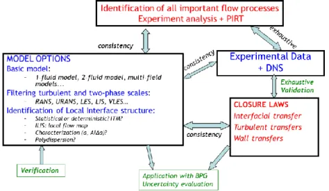
The WG3 proposed the general method illustrated in Figure 3 for using two-phase CFD for NRS problems. The first step is to identify all the important flow processes. This is followed by the selection of the main modelling options, including choosing a basic model (1-fluid, 2-fluid, multi-field), choosing a turbulence model, and deciding on the way to treat the interface(s). Next, the choice of closure laws has to be made, involving how to model the interfacial, turbulent and wall transfers. Finally, there are the verification and validation procedures to follow, as discussed earlier in Section 1. Ideally, if the CFD tool is to be used in the context of a nuclear reactor safety demonstration that uses a best-estimate methodology, one should add a final step: uncertainty evaluation. This may be difficult to fulfil without access to high-performance computing facilities.
Figure 3. General Methodology for Two-Phase CFD Applications to NRS
Most issues with reactors involve complex, two-phase phenomena in complex geometries, and many basic flow phenomena may play a role. The user must identify all these basic thermal hydraulic phenomena before selecting the various modelling options. None of the available CFD codes can be used as a black box in this regard, and the use of a PIRT procedure or something similar, may be the best way to proceed. Here also, a preliminary analysis of experiments simulating the problem (or part of the problem) may be of great help in identifying the phenomena. Given the inherent complexity of any two-phase flow situation, this step may need to be revisited several times during the successive steps of the general methodology. Also, analysing experimental data from the validation matrix may highlight some sensitive phenomena that had not been previously identified. The methodology route may then become iterative.
Three choices are necessary to select the set of balance equations to be used to solve the problem, and they must be consistent with each other. These choices are related to separation into fields, time and space filtering, and the treatment of interfaces (calculated, filtered or statistical). Any two-phase flow situation may be seen as a juxtaposition of several fields and/or phases. The separation into fields is particularly necessary if each field has a velocity and/or temperature significantly different from the others. In some cases, it may be necessary to separate droplets (or bubbles) into several classes of different sizes, especially if their behaviour significantly depends on their size.
The second important choice is the type of time or space averaging, or filtering, to be employed. Pseudo-DNS techniques are still too time-consuming computationally for pragmatic application, and currently can only be used as support to the modelling carried out at more macroscopic scales. Filtered approaches (LES) are also CPU-intensive, but are now within the realms of possibility. RANS-type models are more affordable, and remain the industrial standard for most applications. Depending on the averaging, the interfaces are either tracked directly (i.e. deterministic), filtered, or treated statistically. Two-phase flows have interfaces with a wide range of geometrical configurations. There are locally closed for dispersed fields, e.g. bubbles and droplets, and locally open for free surfaces, a falling film, or a jet. Tracked or filtered interfaces are more appropriate for large interfaces, such as free surfaces or films. A purely statistical treatment is more appropriate for dispersed flows, such as bubbly or droplet flows. In a RANS context, one may need an Identification of the Local Interface Structure (ILIS) to select the appropriate closure laws for the interfacial transfers. Such an ILIS is equivalent to the flow regime map used in 1-D two-fluid models in system codes. A local interfacial structure is defined by three items:
1. the presence of a dispersed gas field (i.e. bubbles) 2. the presence of a dispersed liquid field (i.e. droplets) 3. the presence (and orientation) of a large interface.
In some cases, one may combine a deterministic treatment of large interfaces with a statistical description of the dispersed fields. In a statistical description of interfaces, the interfaces are characterized at least by volume fraction, but very often further information, provided by additional equations, is required for particle number density, interfacial area density, multi-group volume fractions (e.g. the MUSIG model), or any other parameters relating to the particle population.
Any kind of interface may be subject to mass, momentum, and energy interfacial transfer. The formulation of these transfer processes depends on the modelling choices made at previous steps, as described above. If a large interface (such as a free surface) is present, the model may require knowledge of the precise position of this interface, either by using an Interface Tracking Method (ITM) or some other approach. If an ILIS has been used to define the interface structure, the choice of the most appropriate closure laws is then possible. All mass, momentum and energy interfacial transfers have had to have been previously validated on available Separate Effect Tests (SETs). This is also true for the turbulent and wall transfers.
The importance of the verification and validation steps has already been exemplified in Figure 1. The verification step is very difficult to achieve for actual 2-phase flow situations, though the use of numerical benchmarks may be useful to check the viability of the numerical schemes and to measure the accuracy of the solution. A matrix of validation tests (and possibly also demonstration tests) has to be defined and employed. Scoping tests may be necessary to demonstrate the capability of the modelling approach to capture all the important flow processes, at least
qualitatively. Validation tests are then necessary to evaluate the models for interfacial, turbulent, and wall transfer, as far as possible by using SETs.
Guidelines for using Two-Phase CFD
As remarked earlier, two-phase CFD models remain rather immature in comparison with those formulated for single-phase CFD. Nonetheless, as the above example demonstrates, two-phase CFD is being used actively to bring insights into NRS issues for which there is a strong 3-D component to the flow. The WG3 provided some guidance to any potential two-phase CFD analyst, even though the physical models were still under development. Certainly, all the major CFD codes now have two-phase modelling capability, and some help in choosing the most appropriate models is needed.
A general multi-step method of working for using two-phase CFD for safety issues is recommended, as explained below. Following these steps, and being able to justify what is being done at each step, is a good way to demonstrate that the users actually control the whole process and do not simply rely on simulation tools which are still relatively immature. The first step just states that the user should not expect that the CFD code will tell him/her which flow processes will take place in the problem that needs to be studied. The user must himself identify these flow processes, and then check that the simulation tool is able to describe them, either as is, or after some additional developments are made. The second and third steps will exist as long as precise guidelines lack options for selecting the main model and closure relations. The user must elaborate the rationale for these choices for each application.
A number of consistency checks must also be made as elaborated below.
1. The basic choice of the number of fields needed to be adapted to the physical situation, or to an acceptable degree of simplification of it. In particular, if two fields are mechanically and/or thermally uncoupled, and have very different behaviour, they must be treated separately.
2. The averaging procedure needs to give a clear definition of the principal variables, and of the closure terms in the equations. The filtering of the turbulent scales and the two-phase intermittency must be fully consistent.
3. An Interface Tracking Method (ITM) can be chosen, but only if all phenomena having an influence on the interface are also deterministically treated.
4. The choice of an adequate interfacial transfer formulation must be consistent with the selected interface treatment, and with the Identification of the Local Interfacial Structure (ILIS).
5. The SET validation matrix should be exhaustive with respect to all flow processes identified in Step 1, and should be able to validate all the interfacial, turbulent and wall transfers regarded as playing an important role according to Step 1.
6. The number of measured flow parameters in the validation experiments should be consistent with the complexity of the selected model they aim to validate. A model defined by a set of n equations having a set of n principal variables Xi (i = 1, n) can be
said to be clearly “validable” when one can measure n parameters giving the n principal variables.
7. The averaging of measured variables must be consistent with the averaging of the equations.
8. METHODS FOR UNCERTAINTY QUANTIFICATION OF CFD
Code uncertainty methodologies for reactor thermalhydraulics first developed for system codes were based on either “propagation of the uncertainty of input parameters” (so called uncertainty propagation methods) or “accuracy extrapolation” methods (D’Auria & al. , 1995 [22]). A review of methods applicable to CFD was made [9,10].which is here summarized
Methods based on propagation of uncertainties
The method using propagation of code input uncertainties for thermalhydraulics with a link to NRS issues follows the pioneering idea of CSAU [23], later extended by GRS (Glaeser et al., 1994 [24]). It is the most often used class of methods. Uncertain input parameters are first listed including initial and boundary conditions, material properties, and closure laws. Probability density functions are determined for each input parameter. Then the parameters are sampled according to their probability functions and the reactor simulations are run with each set. In the GRS proposal a Monte Carlo sampling is performed with all input parameters being varied simultaneously according to their density function.
The Wilks theorem is often used to treat the results of uncertainty propagation. It makes it possible to estimate the boundaries of the uncertainty range on any code response with a given degree of confidence. The number of code runs is around 100 for an acceptable degree of confidence, even if slightly higher number of code runs, typically 150 to 200 is advisable to have a better accuracy on the uncertainty ranges of the code response.
More generally, propagation of uncertainties typically requires many calculations to reach convergence of statistical estimators which may be difficult with CFD because of large required CPU time. Fortunately, relatively simple statistical tools can give an estimate of the uncertainty resulting from datasets of limited size (bootstrap and Bayes formula for example).
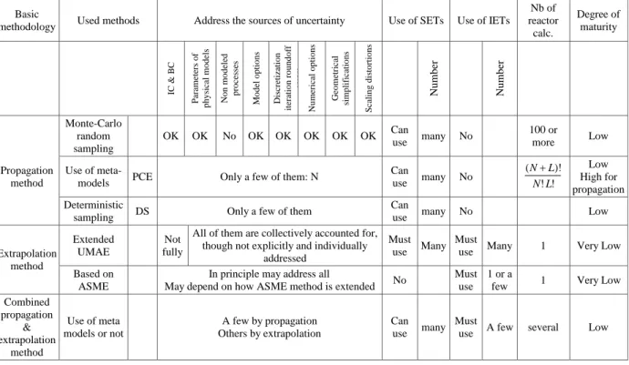
In the domain of uncertainty propagation methods, there are three trends:
The Monte-Carlo type method uses a rather large number of simulations with all uncertain input parameters being sampled according to their pdf. The resulting pdf of any code response is established and the accuracy does not depend on the number of uncertain input parameters.
Use of meta-models: in an attempt to reduce the number of code simulations, some methods consider only the most influential uncertain input parameters and do a few calculations varying these input parameters in order to build a meta-model which will replace the code to determine the uncertainty on any code response with a low CPU cost: the Monte-Carlo method is used with these meta-models, with several thousands of runs. The use of meta-models (such as polynomial chaos expansion and kriging) became popular. These meta-models (or assimilated) provide a mapping between uncertain input parameters and Model results built on a limited number of Model evaluations. They necessarily rely on assumptions of regularity or continuity or shape of Model responses and should be considered with caution when these assumptions are difficult to verify. Basically in such a case, one might replace the non-convergence uncertainty of propagation methods that is rather easy to estimate by uncertainties due to approximations inherent to meta-models which are more difficult to calculate.
Unlike the other two, the deterministic sampling method does not attempt to propagate entire pdfs. Rather it propagates statistical moments. The deterministic samples are chosen such that the known statistical moments are represented. If only the mean and the standard deviation, i.e. the first and second moment, are known, the uncertainty can be represented by two samples. They are chosen such that they have the given mean and standard deviation. Three samples is enough to represent the first four moments of a Gaussian distribution. Arbitrarily higher moments can be satisfied by adding more samples into the ensemble. The method does not suffer from the curse of dimensionality, covariance can also be built into the ensemble, not only the variance of the marginal distributions. The method can be very lean in number of samples, but the challenge lies in finding the right sampling points. Often weighted samples need to be introduced. Also, the assumptions are similar to those necessary for meta-models.
Logically, uncertainty propagation methods require a preliminary work to determine the uncertainties of closure laws. This determination can rely on expert judgment or, for a better demonstration, on statistical methods based on various validation calculations. It may be easy to determine the uncertainty band or pdf for each closure when data are available which are sensitive to a single closure law. This is a separate-effect test in the full sense. In practice very often data are sensitive to a few closure laws and methods have been developed to determine uncertainty bands or pdf for several closure laws based on several data comparisons with predictions (see de Crécy and Bazin, 2004 [25]).
Accuracy extrapolation methods
For system codes, the methods identified as propagation of code output errors are based upon the extrapolation of accuracy. One can cite UMAE (D'Auria and Debrecin, 1995 [22]) and CIAU (D’Auria & Giannotti, 2000 [26], see also Petruzzi & D’Auria, 2008 [27]). A very extensive validation of system codes on both SETs and IETs allows the measurement of the accuracy of code predictions in a large variety of situations. In the case of UMAE and CIAU a metrics for accuracy quantification is defined using Fourier Transform. The experimental data base includes results from different scales and once it is assumed that the accuracy of code results does not depend on the scale this accuracy is extrapolated to reactor scale.
Methods based on extrapolation from validation experiment possibly require only one reactor transient simulation but many preliminary validation calculations of IETs are required.
The ASME V&V20
ASME V&V20 standard for verification and validation in computational fluid dynamics and heat transfer [28] states that: “The concern of V&V is to assess the accuracy of a computational simulation.” This view is clearly compatible with the principle of the methods based on extrapolation from validation experiment.
In current industrial CFD modelling (non DNS), results come from a solved part of Navier-Stokes equations and from a modelled part of these equations. Verification of correct solving of equations can be considered “tractable” even for complex flows and once it is done, physical model uncertainty is a legitimate concern.
Indeed, it is a known fact that different experiments tend to give significantly different model parameters values in a calibration process, which indicates that the form and the generality of the model itself is to be questioned.
Comparison of methods
Methods based on validation results extrapolation offer poor mathematical basis but the confrontation to reality (even in scaled experiments) may give an idea of the impact of model inadequacy on results at full scale. Even the impact of non-modelled phenomena is taken into account when we compare simulations to experiment which is not so clear for uncertainty propagation. Obviously, transposition of results from scaled experiments to full scale is almost impossible to justify rigorously whatever method is used. If we were able to estimate precisely the physical model uncertainty we would also be able to define a perfect model.
Another difference among both methods, propagation and extrapolation, is the possibility to perform sensitivity analysis. Methods based on propagation allow such an analysis by using the results of the runs already performed for the uncertainty analysis. It is impossible with methods based on extrapolation, since they do not consider individual contributors to the uncertainty of the response.
Benchmarking with system codes of the methods belonging to the two different classes was made within the international projects launched by OECD/CSNI. These are identified as UMS (OECD/CSNI. 1998 [0]) and BEMUSE (de Crécy et al. 2007 [30]). A significant lesson of these benchmarks is that the methods have now reached a reasonable degree of maturity, even if the quantification of the uncertainty of the closure laws stays a difficult issue for propagation methods.
The role of Validation in the UQ process
All types of thermalhydraulic codes including system codes and CFD codes use some kind of averaged equations. Local instantaneous equations (continuity, Navier-Stokes and energy equations) are exact equations but they cannot be solved directly due to an excessive CPU cost. Averaging (either time averaging or space averaging or both) is necessary to reduce the time and/or space resolution to a degree that makes the calculation reasonably expensive. However due to the averaging some terms of the equations require some modelling to close the system of equations. Such relations are usually obtained by some theoretical derivation plus some fitting on appropriate experimental data. Such models are approximations of the physical reality and cannot provide exact prediction of the averaged flow parameters. One can then try to estimate the domain of uncertainty of these models or closure relations by using the same data basis and by finding the multiplier values which allow predicting an upper and a lower bound of the data. This may result in a pdf for the multiplier.
This process may be done using separate effect tests in which one particular model (or closure law) is sensitive. In other SETs, measured parameters may be sensitive to a few models. In some cases if there are various flow parameters which are measured, one can identify the sensitivities to each influential model and determine the uncertainty of each model.
In IETs or CETs all models of the code may have some influence on the parameters of interest. It is very difficult to estimate the relative weight of each model in a simulation of the IET. Such IETs may be useful in the UQ process if they simulate the reactor transient of interest. One may consider that the sensitive models and the relative weight of each sensitive model are similar in the IET and