Convex formulations of radius-margin based
Support Vector Machines
Huyen Do [email protected]
Computer Science Department, University of Geneva, Switzerland
Alexandros Kalousis [email protected]
Business Informatics, University of Applied Sciences Western Switzerland
Abstract
We consider Support Vector Machines (SVMs) learned together with linear trans-formations of the feature spaces on which they are applied. Under this scenario the radius of the smallest data enclosing sphere is no longer fixed. Therefore optimizing the SVM error bound by considering both the radius and the margin has the potential to deliver a tighter error bound. In this pa-per we present two novel algorithms: R-SVM+
µ—a SVM radius-margin based feature selection algorithm, and R-SVM+— a met-ric learning-based SVM. We derive our algo-rithms by exploiting a new tighter approxi-mation of the radius and a metric learning in-terpretation of SVM. Both optimize directly the radius-margin error bound using linear transformations. Unlike almost all existing radius-margin based SVM algorithms which are either non-convex or combinatorial, our algorithms are standard quadratic convex op-timization problems with linear or quadratic constraints. We perform a number of experi-ments on benchmark datasets. R-SVM+
µ ex-hibits excellent feature selection performance compared to the state-of-the-art feature se-lection methods, such as L1-norm and elastic-net based methods. R-SVM+ achieves a significantly better classification performance compared to SVM and its other state-of-the-art variants. From the results it is clear that the incorporation of the radius, as a means to control the data spread, in the cost function has strong beneficial effects.
Proceedings of the 30th International Conference on Ma-chine Learning, Atlanta, Georgia, USA, 2013. JMLR: W&CP volume 28. Copyright 2013 by the author(s).
1. Introduction
SVMs (Vapnik, 1998; Cristianini & Shawe-Taylor,
2000) are one of the most popular learning algorithms in machine learning. They have strong theoretical foundations and achieve excellent performance in var-ious applications. They have been used extensively in the context of classification and regression but also for feature selection and weighting (Guyon et al., 2002;
Weston et al.,2000;Rakotomamonjy,2003;Do et al.,
2009b) or Multiple Kernel Learning (Chapelle et al.,
2002; Do et al., 2009a). Their error bound is a func-tion of the ratio of the radius of the smallest sphere containing all data and the margin. However, the opti-mization problems used in standard SVM algorithms rely only on the margin because for a given feature space the smallest sphere enclosing the data is fixed and so is its radius which can thus be safely ignored. Nevertheless, in the context of feature selection or fea-ture weighting the feafea-ture space is transformed and therefore the sphere and its radius are no longer fixed. Thus if we optimize over both the margin and the radius in an SVM-based feature selection or feature weighting scenario we can expect to achieve a tighter generalization error bound which can lead to a better performance. There has been some work that consid-ered this problem, (Weston et al., 2000; Rakotoma-monjy, 2003; Do et al., 2009b). In this context sev-eral radius-margin based SVMs —SVM variants that consider both the margin and the radius of the SVM radius-margin bound, have been proposed. However, due to the challenge set forth by the non-convexity of the radius-margin ratio and the combinatorial na-ture of feana-ture selection, the problem has only been partially solved. Recently,Do et al.(2009b) proposed R-SVM, an SVM variant based on a convex relaxation of the radius-margin ratio. The main drawbacks of R-SVM are that its radius approximation is not opti-mal and that the relaxation on which it is based does
Published in proceedings of the 30th International Conference on Machine
Learning, 2013, Atlanta, USA, pp. 169-177 which should be cited to refer to
this work
not always result to a good approximation of the real radius-margin ratio.
In this paper we address both limitations of R-SVM. We first propose a new tight approximation of the ra-dius which has better properties than the one used in (Do et al., 2009b). Under a geometric interpreta-tion of the radius-margin ratio based error bound, and the recently unveiled metric learning interpretation of SVM (Do et al.,2012), we propose to replace the ratio by the sum of the radius and the inverse of the mar-gin which reflects the same intuition as the orimar-ginal error bound. Moreover, we show that the two formu-lations, ratio-based and sum-based, are equivalent for proper parameter choices. We derive two new convex algorithms which we call R-SVM+ and R-SVM+
µ. R-SVM+ is a Quadratically Constrained Quadratic Pro-gramming optimization problem (QCQP), it is closer to the original SVM formulation since it contains a single set of variables, w. The second algorithm, R-SVM+
µ, is a standard convex quadratic optimization problem with linear constraints. In addition to w, R-SVM+µ contains an explicit feature scaling factor given by µ, on which a sparsity constraint is imposed. The result of the sparsity constraint is that R-SVM+µ performs feature selection. Moreover, we also show how to kernelize both R-SVM+ and R-SVM+
µ. Our new feature selection method, R-SVM+
µ, outperforms the state-of-the-art feature selection algorithms, such as SVMRFE, elastic-net SVM. The R-SVM+achieves state-of-the art classification results and outperforms SVM as well as its variants which make use of data spread measures in their cost function.
The rest of the paper is organized as follows: in the next section we briefly review related work and the original R-SVM. In Section3we describe a new, better approximation of the radius than the one used in R-SVM. In Section4 we describe the optimization prob-lems of R-SVM+ and R-SVM+µ, we show how to solve them in Section 4.5, where we also give their kernel-ized versions. Finally, we present experiments with several benchmark datasets in Section5 and conclude in Section6.
2. Related work
We consider binary classification problems in which we are given a set of training samples S = {(xi, yi)|xi ∈ Rd, y
i ∈ {+1, −1}, i = 1..l}. We denote by kwk2 the `2 norm of w; by w ◦ µ the pairwise product of the two vectors w and µ; and by √µ the element wise application of the square root over the elements of the µ vector.
There are several feature selection criteria based on SVM. SVMRFE, (Guyon et al., 2002), recursively eliminates features with the smallest weights wi. (
We-ston et al., 2000) used the SVM radius-margin ra-tio as a criterion to select features, by minimizing f (σ) = Rγ2(σ) over σ where σ ∈ {0, 1}d which in-dicates that the σi feature is selected or not. This combinatorial optimization problem was relaxed to an integer programming problem, however this relaxed problem is still non-convex. (Rakotomamonjy, 2003) proposed several SVM based criteria to rank features, among them there are criteria based on the radius-margin SVM error bound, which results again in dif-ferent non-convex optimization problems. (Do et al.,
2009b) proposed R-SVM, which directly optimized the radius-margin bound with an additional scaling factor. R-SVM does feature selection and ranking. Similar to that paper, we are interested in a convex relaxation of the radius-margin bound in order to do feature selec-tion; we will describe in more detail R-SVM at the end of this section.
In addition to the feature selection work described above, there have been efforts that try to improve the performance of standard SVM by optimizing the margin and some measure of the data spread, ( Shiv-aswamy & Jebara,2010), (Do et al., 2012); note here that the radius is a natural measure of the data spread. However none of the measures proposed there can be seen as a replacement of a radius-margin-based mea-sure since they are not equivalent (for more on that see in the Appendix). While there is no reason to be-lieve that there is an a-priori ideal measure of the data spread (this would probably depend on the specifici-ties of any given learning problem, and can only be seen on a case by case basis) using the radius has the advantage of the theoretical support it enjoys through its direct reliance on the SVM theoretical error bound. In section4.2we will show how to directly control the radius-margin ratio without using the scaling factor that is used in the feature selection scenarios.
R-SVM: We now briefly review the R-SVM algorithm (Do et al., 2009b). R-SVM uses a feature weighting schema under which the feature space is first scaled by a√µ vector, and then SVM is applied on the resulting feature space. This feature scaling can be expressed by a diagonal linear transformation matrix D√
µ whose diagonal elements are given by √µ; the image of an instance x is given by D√
µx. Under this transfor-mation the feature space is no longer fixed, and the radius of the smallest sphere containing all instances is a function of µ. We denote the radius of the scaled feature space by Rµ.
The motivation of R-SVM was two-fold: first to per-form feature selection in the SVM context, and sec-ond to optimize directly the margin-radius SVM error bound in a ’weighted’ feature space aiming at a better generalization error compared to that achieved by op-timizing only the margin. To do so, the authors opti-mize the radius-margin ratio based SVM error bound, which leads to the following optimization problem1:
min w,b,µ,Rµ 1 2kwk 2 2R2µ (1) s.t. yi(hw, √ µ ◦ xii + b) ≥ 1, ∀i d X k=1 µk= 1, µk≥ 0, ∀k
where Rµ is computed as (Vapnik,1998): min Rµ,x0 R2µ s.t. k √ µ ◦ xi− √ µ ◦ x0k2≤ Rµ2, ∀i (2)
This optimization problem performs smooth feature selection, since the l1 norm constraint on µ leads to a sparse µ solution. However its main limitation is that it is not convex. Therefore the authors proposed to use an upper bound of the objective function by using a linear approximation that upper bounds the radius as maxkµkR2k ≤ R
2 µ ≤
Pd
kµkR2k, where Rk is the ra-dius of the projected instances on dimension k. Using this radius approximation, the authors were able to de-rive a convex upper bound of the objective function of (1) and finally the approximate optimization problem was: min w,b,ξ,µ 1 2 d X k hwk, wki µk +PdC kµkR 2 k l X i ξi2 (3) s.t. yi( d X k hwk, Φk(xi)i + b) ≥ 1 − ξi d X k=1 µk= 1, µk≥ 0, ∀k
However, this optimization problem has two limita-tions. First, it uses two levels of approximation, one for the radius and one for the objective function (i.e using the upper bound of the real objective function). Second, it cannot be kernelized due to the use of the radius approximation, thus limiting the application of R-SVM only to the original feature space. The same radius approximation has also been used by (Do et al.,
2009a) in the context of multiple kernel learning. In the next section we will derive a new approximation of the radius with better properties than the one pro-posed in (Do et al., 2009b). Later we will also show how to address the kernelization problem.
1Note that√µ◦x = D√
µx and depending on our needs
we will use interchangingly one or the other.
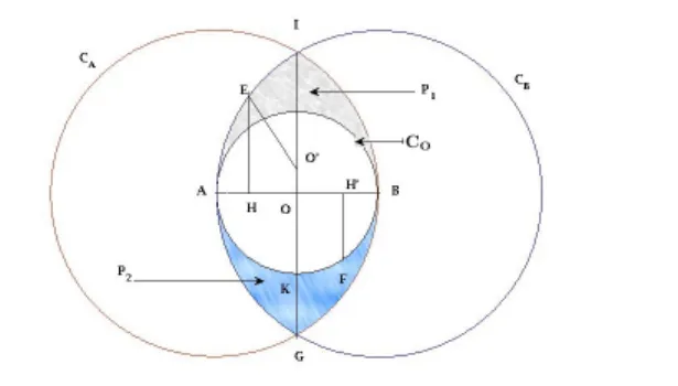
Figure 1. Demonstrating the radius relations.
3. A better approximation of the radius
The main disadvantage of the upper bounding linear approximation of the radius used in (Do et al.,2009b), i.e. R2µ ≤ Pd
kµkR2k, is that we cannot quantitatively estimate its approximation error, which, depending on the dataset, can be very large. Here we propose a bet-ter radius approximation, the error of which we can estimate quantitatively. The main idea is to approx-imate the radius of the smallest sphere enclosing the data, R, by the maximum pairwise distance over all pairs of instances. Our new radius approximation, i.e the half value of the maximum pairwise distances, RO, is tighter than the approximation used in (Do et al.,
2009b) and can be estimated quantitatively, where RO≤ R ≤ 1+
√ 3
2 RO≈ 1.366RO.
Let R be the radius of the smallest sphere C containing all instances. Let xA, xB, be the two instances which have the maximum distance d. We denote by xO the point given by xO = xA+x2 B, i.e. the middle point on the line segment defined by xA and xB. CB is the sphere with center xB and radius RB = d, CA is the sphere with center xA and radius RA = d, and CO is the sphere with center xO and radius RO= d/2. This configuration for the two dimensional space is given in Figure 1. All instances lie within the intersection of the CA and CB spheres since kxi− xAk ≤ d, ∀i and kxi− xBk ≤ d, ∀i. Therefore the CO sphere encloses most instances except the ones that are inside the in-tersection of the CB and CAbut outside CO, hence we have RO ≤ R. We prove the following inequality (see details in Appendix).
Lemma 1: The inequality RO ≤ R ≤ 1+ √
3
2 RO holds for any two or higher dimensional space.
From now on we denote by r the quantity (2RO)2= d2, which corresponds to the squared diameter of the CO sphere and the maximum squared distance be-tween any two instances. The new algorithms that we present use this quantity instead of the traditional radius. Thus instead of controlling directly the R ra-dius of the smallest sphere enclosing the instances we
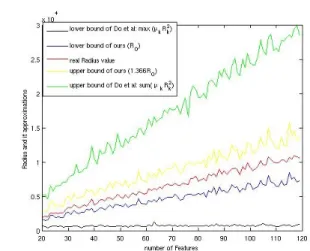
Figure 2. Demonstrating the squared radius and its two approximations. The red line is the real value of the ra-dius. The range between black and green lines, which cor-responds to the approximation by sum squared radius com-ponents, are much larger than that between blue and yel-low lines, which corresponds to the approximation by the squared half of maximum pairwise distance.
control the square of the maximum distance between any pair of instances. As a result we eventually replace the optimization problem used to compute the radius, given in (2), by the following simple one:
min r r s.t. k √ µ ◦ xi− √ µ ◦ xjk2≤ r, ∀i, j (4)
Note that (4) is simply a formal way to formulate the maximum distance between instances, formula-tion which will be useful in the upcoming secformula-tions. We should note that our radius approximation reflects closely the true radius. If for example the latter might be distorted by outliers so will be our approximation. This raises the interesting problem of extending the margin-radius SVM theory to capture the soft radius in which outlier instances will be addressed through slack variables.
3.1. Comparison to existing radius
approximations and the real radius value
Do et al.(2009b) proved that the inequality:
max k µkR 2 k ≤ R 2 µ≤ d X k µkR2k≤ max k R 2 k (5)
holds; this inequality provides a range within which the radius value will vary. However they could not show how close this approximation is, i.e. the linear sumPd
kµkR2k to the real radius value, R 2
µ. Therefore the only criterion for evaluating the accuracy of this approximation is via the range between maxkµkR2k
andP
kµkR2k. We will show theoretically and demon-strate empirically that our new approximation range RO≤ Rµ≤ 1.366RO is more accurate than the one of (Do et al.,2009b).
In (5), the squared radius is bounded by maxkµkR2k and maxkR2k. We see that the range between maxkµkR2k and maxkR2k can be very large, from
1
d ∗ 100% to 100% of maxkµkR 2
k, since the possible minimum value of maxkR2k is maxkµkR2k/d when µ is uniform and Rk are all equal. Even if Rk are dif-ferent, when µ is uniform, the ratio maxkµkRk
P
kµkR2k
will be equal to maxkRk
P µkR2k
which can be also very small espe-cially for high dimensional data (where d is large). Unlike this as we have shown our new approximation ROcan be estimated quantitatively and is quite tight, RO≤ Rµ≤ 1.366RO.
Moreover, since minkR2k ≤ P
kµkR2k ≤ maxkR2k, R-SVM will not work if the component radii Rk are roughly equal. In that caseP
kµkR2k is almost a con-stant for any µ,P µk = 1, µk≥ 0. However this does not mean that the real value of the radius is also a constant when µ is varied.
Empirical comparison: We generate randomly 1000 data points using gaussian distributions with dif-ferent number of features (from 20 to 120) and keep µ equal to 1. Figure 2 shows the value of the squared ra-dius, its two approximations and their ranges. We see that our radius approximation has an even stronger advantage over the one used in (Do et al., 2009b) as the number of features increases.
4. Two new variants of radius-margin
based SVM
The SVM error bound implies that the larger the mar-gin and the smaller the radius are, the better the gener-alization error will be. We can transform—scale—the original feature space and subsequently find a sepa-rating hyperplane in the transformed feature space so that the radius is minimized and the margin is maxi-mized, as it was done in the original R-SVM. Through the radius we control the spread of the instances. Re-cently, Do et al.(Do et al., 2012) have given a new interpretation of SVM from a metric learning perspec-tive. Under this view the SVM algorithm can be de-scribed as follows. Given instances in the feature space H, we linearly transform H with the help of the di-agonal linear transformation W, diag(W) = w, and then translate by a value b, so that the linearly trans-formed instances are placed optimally and symmetri-cally around the fixed hyperplane H1: 1Tx + 0 = 0.
Under this view the radius can be seen as a measure of the total data spread, and the margin as a measure of the between class distances. So the SVM radius-margin bound conforms with one of the basic biases of metric learning: maximizing the between class dis-tances while minimizing the within class disdis-tances. Exploiting this new insight of SVM, we can explicitly control the margin and the data spread by not only using the radius-margin ratio but other functions such as the sum of the radius and the inverse of the mar-gin. Later we will show that the two cost functions, the sum and the ratio, are in fact equivalent under proper parameter choices.
We will now present two new algorithms, R-SVM+ µand R-SVM+; both of them optimize the radius-margin sum cost function. R-SVM+
µ is an adaptation of the original R-SVM optimization problem. It uses the sum in its cost function as well as the new radius approx-imation. It relies on two sets of variables, w which corresponds to the SVM linear classifier, and µ which is a sparse feature weighting, that corresponds to the diagonal transformation D√
µ under which the SVM gives the best results. Thus in addition to the radius-margin optimization, R-SVM+µ, due to the sparsity im-posed on µ, performs also feature selection. R-SVM+ also makes use of the sum cost function and the new ra-dius approximation. Unlike R-SVM+
µ, it uses a single set of variables to learn the best diagonal linear trans-formation that optimizes the ratio and margin bound; w = diag(W) describes both the hyperplane and the scaling of the feature space. R-SVM+ only optimizes the radius-margin sum cost function, it does not do feature selection since there is no sparsity constraint on the features.
4.1. R-SVM+µ
As we already mentioned R-SVM+µ is an adaptation of the optimization problem of the original R-SVM in which the ratio is replaced by the sum; its exact form is: min w,ξ,µ,b,Rµ,x0 1 2kwk 2 2+ λR 2 µ+ C l X i ξi (6) s.t. yi(hw, D√µxii + b) ≥ 1 − ξi, ∀i d X k=1 µk= 1, µ, ξ ≥ 0 kD√ µxi− D√µx0k2≤ R2µ, ∀i
This optimization problem is non-convex and diffi-cult to solve because of the constraints related to the radius (2). Fortunately we can reformulate it as a con-vex problem by replacing the original radius Rµby its tight approximations given by (4). The relaxed convex
optimization problem is 2: min w,b,ξ,µ,r 1 2 d X k w2k µk + λr + C l X i ξi (7) s.t. yi( d X k hwk, xiki + b) ≥ 1 − ξi, ∀i; d X k=1 µk= 1 1 2kD √ µxi− D√µxjk2≤ r, ∀i, j; µ, ξ ≥ 0 We have wk2
µk is convex; and since kD
√ µxi − D√
µxjk2=Pdkµk(x2ik+ x2jk− 2xikxjk), the last con-straint of (7) is linear with respect to µ and r. Hence (7) is a convex optimization problem.
Similar to SVM, R-SVM+µ can also be seen under a metric learning view. It first learns a diagonal lin-ear transformation D√
µ and then a linear transfor-mation W and a translation b so that the transformed instances are placed optimally around the fixed hy-perplane H1, while keeping the radius of the smallest sphere containing the transformed instances small. 4.2. R-SVM+
In this section, we propose an algorithm to improve the standard SVM by directly controlling the radius-margin error bound without making use of the scaling factor µ. Note that in the standard view of SVM, the only way to explicitly control the radius is to use a second set of variable µ, as it is done in R-SVM and R-SVM+µ. The D√µ variable linearly transforms the H feature space and controls the radius of the enclos-ing sphere, without it the radius is a fixed predefined value. However, under the metric learning view we no longer need D√
µ to control the radius. We can con-trol both the radius and the margin via W. Dropping the D√
µ variable and controlling the radius and the margin via W results in the R-SVM+ optimization problem which is:
min w,b,ξ,Rw,x0 1 2kwk 2 2+ λR 2 w+ C l X i ξi (8) s.t. yi(hw, xii + b) ≥ 1 − ξi, ξi≥ 0, ∀i kWxi− Wx0k2≤ R2w, ∀i Unlike R-SVM+
µ this formulation does not perform feature selection, since it no longer uses the µ variable together with the l1 constraint that played that role. The advantage of this formulation is that it directly controls the radius and margin error bound which can lead to better predictive performance. This formula-tion is also in accordance with several metric learn-ing algorithms, in which the data spread is kept small while the between class distance is maximized. In our
2We rewrite w :=√µ ◦ w, so we have w k=
√ µ
formulation the radius corresponds to the data spread and the margin corresponds to the between class dis-tance.
Nevertheless, this optimization problem is not convex either. We derive a new relaxed formulation of R-SVM+by replacing in (8) the radius R
wcomputed by (2) with the r approximation (4) and get the following optimization problem: min w,ξ,b,r 1 2kwk 2 2+ λr + C l X i ξi (9) s.t. yi(hw, xii + b) ≥ 1 − ξi, ξi≥ 0 1 2kWxi− Wxjk 2 ≤ r, ∀ij We have kWxi − Wxjk2 = P d kw 2 k(x 2 ik + x 2 jk − 2xikxjk) = wTPw, where P is a diagonal matrix with elements (xik−xjk)2. Therefore P is positive semidefi-nite and the last constraint of (9) is convex. Hence the optimization problem (9) is a QCQP problem. We can solve the optimization problem (9) in the primal form. However, due to the limitations of the existing QCQP solvers which can deal with only a small number of constraints and variables, we can have computational problems because (9) has n × (n + 1)/2 constraints; we thus propose to solve it in its dual form (Section4.5). 4.3. Two transformations vs one
From a metric learning perspective, both R-SVM+µ and R-SVM+ learn diagonal linear transformations and a translation b which maximize the margin w.r.t the fixed hyperplane H1 and minimize the radius, i.e the data spread. R-SVM+
µ learns two linear transfor-mations, W and D√
µ, diag(D√µ) =
√
µ or WD√ µ
; R-SVM+ learns only one linear transformation W. D√
µcontrols the sparsity of the feature selection (since
P µk= 1, µk≥ 0). LearningWD√µwill first transform
the feature space to a more sparse (lower rank) space, on which a non regularized diagonalWis then learned. In R-SVM+
µ the radius is only considered by theD√µ
transformation but not by theW. In R-SVM+the ra-dius is considered in the full transformed space given byW.
4.4. Equivalence of the sum and the ratio forms
We will show that optimizing the radius-margin ratio, kwk2R2, e.g in problem (1), is equivalent to optimizing the radius-margin sum kwk2+ λR2, e.g in problems (6,8), under some proper choice of λ. Without loss of generality we consider the following two optimization
problems: min w,R kwk 2 R2 s.t w, R ∈ F (10) min w,R kwk 2 + λR2 s.t w, R ∈ F (11) where F is some feasible set. The following lemma indicates that those are equivalent with some proper choice of parameter λ (see proof in Appendix)3.
Lemma 2. For each optimal solution of the ratio form (10), there exists a value of λ for which, the sum form (11) has the same optimal solution.
4.5. Solving the convex optimization problems of R-SVM+µ and R-SVM+
The details of how to solve the R-SVM+µ and R-SVM+ optimization problems can be found in Ap-pendix. Since both are convex, a general interior point method can work well, however, the number of con-straints may be problematic on large problems. There-fore, we propose to use an efficient two-step approach with gradient descent to solve them. In short, our method can deal with the constraints of the radius efficiently, since we have to compute the pairwise in-stance diin-stances only once, and at each iteration, we just have to compute the inner product of two vectors to handle all the constraints on the radius.
4.6. Kernelization
Given a kernel function K corresponding to a fea-ture mapping x ∈ Rd 7−→ Φ(x) ∈ H, we show how R-SVM+ and R-SVM+
µ can be applied in the feature space H. The kernelization of R-SVM+ and R-SVM+
µ is based on the idea of a proximity space representation in which learning instances are repre-sented by their similarities or distances with respect to a set of instances (Pekalska & Duin, 2005). In R-SVM+ we parametrize the diagonal scaling ma-trix W using the same trick as in metric learning (Torresani & Lee, 2006; Goldberger et al., 2005), i.e
f
W = WΦ(X) where Φ(X) is the matrix the i row of which is Φ(xi). R-SVM+µ can be kernelized in the same way as R-SVM+, where instead of parametriz-ing matrix W, we parametrize eD√
µ = D√µΦ(X). In fact this kernelized form corresponds to the application of the R-SVM+ or R-SVM+µ in the proximity space in which an instance xi is represented by the vector Ki = (K(xi, x1), . . . K(xi, xn))T, i.e. the i column of the kernel matrix, we can thus solve it by simply
ap-3See complimentary document for detailed proofs
re-lated to our new radius approximation, the lemmas, how to solve our optimization problems, another way of kernel-izing R-SVM+, and other additional arguments.
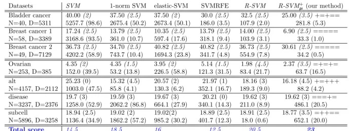
Table 1. First line per dataset: Classification error(%) and McNemar score in parentheses. Second line: average number of selected features and percentage of selected features in parentheses. N is the number of instances and D the dimensionality of each dataset. (+) means our methods significantly better than the previous methods, (=) means they are equal.
Datasets SVM 1-norm SVM elastic-SVM SVMRFE R-SVM R-SVM+
µ (our method) Bladder cancer 40.00 (2) 37.50 (2.5) 37.50 (2 ) 30.0 (2.5) 32.5 (2.5) 25.00 (3.5) +=+== N=40, D=5311 5257.7 (98.6) 2675.4 (50.2) 2673.4 (50.1) 186.0 (3.5) 107.9 (2.0) 281.8 (5.3) Breast cancer 1 17.24 (2.5) 13.79 (2.5) 10.35 (2.5) 13.79 (2.5) 14.00 (2.5) 6.90 (2.5) ===== N=58, D=3389 3168.6 (93.5) 361.0 (10.7) 597.4 (17.6) 318.1 (9.4) 103.9 (3.1) 33.3 (1.0) Breast cancer 2 36.73 (2.5) 34.70 (2.5) 40.82 (2.5) 40.82 (2.5) 36.73 (2.5) 30.61 (2.5) ===== N=49, D=7129 4202.2 (58.9) 743.7 (10.4) 1694.3 (23.8) 341.7 (4.8) 554.9 (7.8) 34.2 (0.5) Ovarian 4.35 (2) 4.35 (1.5) 3.95 (2) 5.14 (1.5) 1.98 (4.5) 2.37 (3.5) =+=+= N=253, D=385 152.0 (39.5) 53.2 (13.8) 226.5 (58.8) 121.3 (31.5) 83.4 (21.7) 63.7 (16.5) alt 25.23 (0) 15.32 (4.5) 20.57 (2) 21.97 (1) 18.16 (3) 16.18 (4.5) +=+++ N=4157, D=2112 1003.0 (47.5) 85.8 (4.1) 130.3 (6.2) 352.1 (16.7) 189.3 (9.0) 88.2 (4.2) disease 19.7 (3) 19.59 (3) 19.67 (3) 20.21 (0) 19.62 (3) 19.62 (3) ===+= N=3237, D=2376 1258.0 (52.9) 2062.2 (86.8) 664.1 (27.9) 340.1 (14.3) 211.0 (8.9) 486.1 (20.5) subcell 18.94 (2.5) 19.02 (2) 19.02(2) 18.89 (2.5) 18.91 (2.5) 18.77 (3.5) =++== N=5896, D=3258 1136.4 (34.9) 1862.2 (57.2) 985.2 (30.2) 401.7 (12.3) 18.0 (0.6) 652.1 (20.0) Total score 14.5 18.5 16 12.5 20.5 23 plying R-SVM+or R-SVM+
µ in this proximity space.
5. Experiments
We performed two sets of experiments. In the first we focused on the feature selection task of our new feature selection algorithm R-SVM+
µ; and in the second on the classification task of our new rank-one metric learning algorithm R-SVM+ as well as the kernelized versions of R-SVM+, R-SVM+
µ and R-SVM.
Feature selection: We did the feature selection ex-periments on high dimensional biological datasets and text datasets (Kalousis et al., 2007). Attributes are standardized to zero mean and unit variance. We com-pare our method,R-SVM+µ, with 1-norm SVM (Zhu et al.,2003), elastic-net SVM (Wang et al.,2006;Zou & Hastie, 2005; Ye et al., 2011) (both 1-norm SVM and elastic-net SVM use the L1 norm constraint on w) and SVMRFE (Guyon et al., 2002), one of the most popular feature selection methods. We also com-pare with R-SVM (Do et al.,2009b), the recent radius-margin SVM based feature selection algorithm. In ad-dition to comparing with the popular feature selection algorithms, we also use a linear SVM to have an in-dication of the baseline performance with no feature selection. For SVMRFE we chose k, the number of selected features, from [1%, 2%, ..., 100%] of the total number of features by inner cross validation, which clearly incurs a high additional computational cost. For biological datasets, since the number of samples is small, we estimate the error using 10-fold Cross Vali-dation. For text datasets we randomly split the data 30 times, with 300 instances for training and the rest
for testing. To estimate the statistical significance of the error results we used McNemar’s test for 10-fold CV and used t-test for the random-split estimation, both with a significance level of 0.05. To compare all algorithms over several datasets, we used the following scoring schema: if algorithm A is significantly better than algorithm B, then A gets one point and B zero, if there is no significant difference both get 0.5 points. For a given dataset, the score of each algorithm is the sum of its score in all pairwise comparisons. We se-lect the C and λ hyperparameters of the algorithms by inner 10-fold CV from the set{0.1, 1, 10, 100, 1000}. In Table 1 we give the error of the six algorithms, as well as the results of the McNemar’s and t-test based scoring. R-SVM+µ is significantly better in two of the seven datasets compared to 1-norm SVM and never significantly worse; it is three times significantly bet-ter than elastic-net SVM and never significantly worse, and finally it is also three time significantly better than SVMRFE and never worse. In terms of the total rank-ing score over all the datasets R-SVM+
µ is ranked on the top with 23 points, followed by R-SVM, 20.5, 1-norm SVM, 18.5, elastic-net SVM, 16, and SVM-RFE, 12.5. What is more impressive is that this systemati-cally better or equivalent classification performance is achieved with a significantly less number of selected features. The number of selected features of R-SVM+µ is often more than an order of magnitude less than the number of features selected by the other feature selection algorithms, especially compared to 1-norm SVM and elastic-net SVM. Note that for some cases, 1-norm SVM and elastic-net SVM fail to select fea-tures, their optimal value is achieved when all features
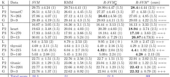
Table 2. Average classification error (%) and standard deviation of SVM, RMM, R-SVM+ and R-SVM+µ in the kernel
spaces. Numbers in parentheses are t-test scores. (+) means our method R-SVM+ significantly better than the previous three methods (SVM, RMM or R-SVM+µ), (=) means they are equal.
K Data SVM RMM R-SVM+ µ R-SVM+(ours) L 29.75 ±4.24 (1) 29.74±4.41 (1) 28.99±4.47 (1.5) 28.4±4.44 (2.5) ++= P2 breastC 26.51 ± 4.52 (1.5) 26.61 ± 4.45 (1.5) 27.27 ±4.45 (1.5) 27 ± 4.33 (1.5) === P3 N=263 27.86 ± 4.07 (1) 27.12 ± 4.11 (1.5) 26.61±4.56 (2) 27.05 ± 4.85 (1.5) === G D=9 29.49 ± 4.19 (1.5) 29.44 ± 4.3 (1.5) 29.83 ±4.11 (1.5) 29.03 ± 4.22 (1.5) === L 16.07 ± 3.05 (1.5) 16.36 ± 3.1 (1.5) 16.44 ± 3.13 (1.5) 16.13 ± 3.33 (1.5) === P2 heart 19.63 ± 3.48 (1.5) 20.04 ± 4.03 (1) 20.39 ±4.03 (1) 18.94 ± 3.74 (2.5) =++ P3 N=270 17.93 ± 3.63 (1.5) 17.91 ± 3.66 (1.5) 18.18± 4.61 (1) 17.10 ± 3.63 (2) ==+ G D=13 30.01 ± 5.37 (1) 29.95 ± 5.24 (1) 30.85 ± 7.29 (1) 26.87±4.73(3) +++ L 8.6 ± 2.53 (2) 8.79 ± 2.53 (2) 9.95 ± 2.6 ( 0 ) 8.19 ± 2.47 (2) ==+ P2 thyroid 4.69 ± 2.11 (1.5) 4.64 ± 2.1 (1.5) 4.49 ± 2.16 (1.5) 4.29 ± 2.12 (1.5) === P3 N=215 5.6 ± 2.45 (0.5) 6.04 ± 2.7 (0.5) 4.32± 2.04 (2.5) 4.4± 1.92 (2.5) ++= G D=140 5.03 ± 2.08 (1) 5.45 ± 2.34 (1) 5.09± 2.24 (1) 4.28 ± 2.13 (3) L 22.71 ± 1.51 (1.5) 22.76 ± 2.56 (1.5) 22.7 ± 1.51 (1.5) 22.91 ± 2.02 (1.5) === P2 titanic 23.21 ± 1.29 (1.5) 23.06 ± 1.58 (1.5) 23.04 ± 1.22 (1.5) 22.93 ± 1.22 (1.5) === P3 N=2201 22.77 ± 0.92 (1) 22.66 ± 0.82 (1.5) 22.74 ± 1.23 (1.5) 22.42 ± 1.24 (2) +== G D=3 22.76 ± 1.37 (1) 22.62 ± 0.92 (1) 22.84 ± 0.91 (1) 22.32 ± 0.79 (3) +++ Total score 20.5 21 21.5 33
have equally a zero coefficient, and only the bias plays a role in the separating hyperplane.
Classification: Here we examine the predictive per-formance of SVM when we incorporate the SVM ob-jective function with some measure of the data spread, namely the radius. We evaluate the performance of our two SVM variants, R-SVM+ and R-SVM+
µ, and com-pare them to standard SVM and RMM (Shivaswamy & Jebara, 2010). The latter is an SVM variant that, in addition to the margin, controls also a measure of the data spread. We do the comparison on the same benchmark datasets used in (Shivaswamy & Jebara,
2010) and (Ratsch et al.,2001).
We used the same 100 random splits as in these two papers, and tested the statistical significance by t-test at 5% significance level. The scoring schema is the same as in the feature selection experiments. We ex-perimented with three types of kernel: linear (L), poly-nomial with degree two (P2), polypoly-nomial with degree three (P3) and the gaussian with σ = 1 (G). We nor-malized the kernels to have a trace of one. The B parameter of RMM is chosen by inner cross valida-tion from {0.1, 1, 10, 100, 1000}. We report the error results and the t-test’s scores in Table2. R-SVM+ is the best with 33 points compared to 21.5 of R-SVM+
µ, 21 of RMM and 20.5 of SVM. The better predictive performance of R-SVM+ over SVM can be explained by the fact that we directly optimize both the radius and the margin in the SVM error bound in a linearly transformed space. Therefore from a metric learn-ing view R-SVM+ is more flexible than SVM, i.e it controls both the within- and between-class distances
while SVM controls only the between class distances (the margin).
6. Conclusion
We introduced two new convex formulations of the radius-margin based SVM, R-SVM+
µ and R-SVM+. Both are based on a new tight radius approximation, the approximation error of which we estimate quanti-tatively. R-SVM+
µ uses an explicit feature weighting factor which together with a sparsity constraint re-sults to an inherent mechanism for feature selection It has a better or equivalent a classification performance compared to the state-of-the-art feature selection algo-rithms, namely 1-norm SVM, elastic-net SVM, SVM-RFE. Even more it achieves this performance with a surprisingly high sparsity level. It selects considerably less features, often an order of magnitude less, than the other feature selection algorithms. R-SVM+ can be considered as a new rank-one metric learning al-gorithm, which directly optimizes the radius-margin SVM error bound. Unlike SVM which optimize only the margin, i.e the between-class distance, R-SVM+ optimizes also some within-class distance, which re-sults in a better classifier. Experiments on a number of benchmark datasets shows that R-SVM+ achieves a significantly better classification performance than that of SVM and RMM. The latter, RMM, is an SVM variant which also uses a data spread measure. Finally, we also derived kernelized versions for both R-SVM+ and R-SVM+µ, something that has not been done be-fore for the existing radius-margin based SVM vari-ants.
Acknowledgments
This work was partially supported by the Swiss NSF (Grant 200021-122283/1).
References
Chapelle, O., Vapnik, V., Bousquet, O., and Mukher-jee, S. Choosing multiple parameters for support vector machines. Machine Learning, 46, 2002. Cristianini, N. and Shawe-Taylor, J. An introduction
to Support Vector Machines. Cambridge Uni. Press, 2000.
Do, H., Kalousis, A., Woznica, A., and Hilario, M. Margin and radius based multiple kernel learn-ing. In European Conference on Machine Learning (ECML), pp. 330–343, 2009a.
Do, H., Kalousis, A., Wang, J., and Woznica, A. A metric learning perspective of svm - on the relation of svm and lmnn. In Journal of Machine Learn-ing Research W&C ProceedLearn-ings - AI and Statistics (AISTATS), 2012.
Do, Huyen, Kalousis, Alexandros, and Hilario, Melanie. Feature weighting using margin and radius based error bound optimization in svms. In Eu-ropean Conference on Machine Learning (ECML), 2009b.
Goldberger, J., Roweis, S., Hinton, G., and Salakhut-dinov, R. Neighbourhood components analysis. In Neural Information Processing Systems (NIPS), vol-ume 17. MIT Press, 2005.
Guyon, I., Weston, J., Barnhill, S., and Vapnik, V. Gene selection for cancer classification using sup-port vector machine. Machine Learning, 46:389–422, 2002.
Kalousis, A., Prados, J., and Hilario, M. Stabil-ity of feature selection algorithms-a study on high-dimensional spaces. Knowl. Inf. Syst, 12:95–116, 2007.
Pekalska, E. and Duin, R. The Dissimilarity Repre-sentation for Pattern Recognition. Foundations and Applications. World Scientific Publishing Company, 2005.
Rakotomamonjy, A. Variable selection using svm-based criteria. Journal of Machine Learning Re-search, 3, 2003.
Ratsch, G., Onoda, T., and Muller, K. R. Soft margins for adaboost. Machine Learning, 2001.
Shivaswamy, P. K. and Jebara, T. Maximum relative margin and data-dependent regularization. Journal of Machine Learning Research, 11, 2010.
Torresani, L. and Lee, K. Large margin component analysis. In Neural Information Processing Systems (NIPS), 2006.
Vapnik, V. Statistical learning theory. Wiley InterSc, 1998.
Wang, L., Zhu, J., and Zou, H. The doubly regularized svm. Statistica Sinica, 2006.
Weston, J., Mukherjee, S., Chapelle, O., Pontil, M., Poggio, J., and Vapnik, V. Feature selection for svms. Neural Information Processing Systems (NIPS), 2000.
Ye, G., Chen, Y., and Chen, Y. Efficient variable selec-tion in SVMs via the alternating direcselec-tion method of multipliers. In AI and Statistics, 2011.
Zhu, J., Rosset, S., Hastie, T., and Tibshirani, R. 1-norm support vector machine. In Neural Informa-tion Processing Systems (NIPS), 2003.
Zou, H. and Hastie, T. Regularization and variable selection via the elastic net. Journal of the Royal Statistical Society Series B, 2005.