Development of the trigger menu and search for new phenomena in the dilepton final state with the ATLAS detector at the LHC

(1)

HAL Id: tel-01389876

https://hal.archives-ouvertes.fr/tel-01389876

Submitted on 30 Oct 2016

HAL is a multi-disciplinary open access

archive for the deposit and dissemination of sci-entific research documents, whether they are pub-lished or not. The documents may come from teaching and research institutions in France or abroad, or from public or private research centers.

L’archive ouverte pluridisciplinaire HAL, est destinée au dépôt et à la diffusion de documents scientifiques de niveau recherche, publiés ou non, émanant des établissements d’enseignement et de recherche français ou étrangers, des laboratoires publics ou privés.

Development of the trigger menu and search for new

phenomena in the dilepton final state with the ATLAS

detector at the LHC

Tetiana Berger-Hrynova

To cite this version:

Tetiana Berger-Hrynova. Development of the trigger menu and search for new phenomena in the dilepton final state with the ATLAS detector at the LHC. High Energy Physics - Experiment [hep-ex]. Grenoble 1 UGA - Université Grenoble Alpes, 2016. �tel-01389876�

(2)

LAPP-H-2016-002

Université Grenoble Alpes

Mémoire présenté par

Tetiana Berger-Hryn’ova

pour obtenir le diplôme de

Habilitation à Diriger des Recherches

Spécialité: Physique des Particules

Development of the trigger menu and search

for new phenomena in the dilepton final state

with the ATLAS detector at the LHC

Soutenu le 03/06/2016 devant le jury composé de :

Dr. Stéphane Jézéquel (LAPP, Annecy-le-Vieux) Examinateur Dr. Giovanni Lamanna _{(LAPP, Annecy-le-Vieux)} President du Jury Dr. Fabienne Ledroit-Guillon _{(LPSC, Grenoble)} Rapporteuse

Dr. Emmanuel Perez _{(CERN, Genève)} Examinateur

Prof. David Strom _{(University of Oregon, Eugene)} Rapporteur Dr. Patrice Verdier _{(IN2P3, Paris )} Rapporteur

(3)

(4)

LAPP-H-2016-002

Université Grenoble Alpes

Mémoire présenté par

Tetiana Berger-Hryn’ova

pour obtenir le diplôme de

Habilitation à Diriger des Recherches

Spécialité: Physique des Particules

Development of the trigger menu and search

for new phenomena in the dilepton final state

with the ATLAS detector at the LHC

Soutenu le 03/06/2016 devant le jury composé de :

Dr. Stéphane Jézéquel (LAPP, Annecy-le-Vieux) Examinateur Dr. Giovanni Lamanna _{(LAPP, Annecy-le-Vieux)} President du Jury Dr. Fabienne Ledroit-Guillon _{(LPSC, Grenoble)} Rapporteuse

Dr. Emmanuel Perez _{(CERN, Genève)} Examinateur

Prof. David Strom _{(University of Oregon, Eugene)} Rapporteur Dr. Patrice Verdier _{(IN2P3, Paris )} Rapporteur

(5)

(6)

Chapter 1 Introduction

Elementary particle physics has made remarkable progress in its hundred years of existence. In the Standard Model of particle physics (SM) we have a comprehensive gauge theory of particle interactions which provides accurate predictions for almost all phenomena in high-energy physics. Its current formulation was finalized in the late 1970s - early 1980s with experimental confirma-tion of the existence of quarks [1,2] and W±and Z0 bosons [3,4,5,6]. Since then, the discoveries of the top quark in 1995 [7,8], the tau neutrino in 2000 [9], and more recently the Higgs boson in 2012 [10,11] have given further credibility to the SM. The fundamental parameters of the SM can be fitted to all the relevant measurements and this global electro-weak fit confirms that all the observations are consistent as shown in Figure 1.1.

Despite of its successes, the SM has some shortcomings. It does not contain any viable dark matter candidate that possesses all the properties required by observational cosmology and also fails to explain the matter/anti-matter asymmetry of the universe. It also does not incorporate neutrino oscillations or account for the accelerating expansion of the universe.

Also the SM has 19 arbitrary parameters (or 26 if we include neutrino masses and mixing). The SM fermion mass parameters span five-six orders of magnitude and the reason for those differences is not understood. Also the Higgs boson mass is at the electro-weak scale (∼125 GeV). This mass is subject to radiative corrections of order∆m2

H ∝ Λ2 from quantum loop interactions

with fermions and bosons, where Λ is a the cut-off scale of the theory. If the SM is valid up to the Planck scale (ΛP l), the Higgs mass would be subject to gigantic corrections and the bare

Higgs mass would have to be O(ΛP l). The SM would have to be fine-tuned such that quadratic

terms of this order cancel to within 100 GeV, which spoils the naturalness of the theory. This fine-tuning would not be necessary if there is new physics at the electro-weak scale.

All the above hints that the SM is an effective theory, a low energy approximation valid up to Λ ≈ 1 TeV, of this complete theory, so-called “Theory of Everything”. The nature of this theory is completely unknown, putting us in a unique situation which we have not had for over 50 years now, where we are searching blindly, without any guidance from the theory. Only data can provide us answers to our questions and hopefully bring positive surprises. We are fortunate to possess the tools needed to collect this data, with the Large Hadron Collider (LHC) at the European Organization for Nuclear Research (CERN) and its experiments.

The LHC was proposed in early 1990s with the aim “to produce, not only high energy but a higher luminosity... than existing or planned hadron colliders” [13]. The main constraints on the LHC configuration were brought by the existing tunnel of the Large-Electron-Positron collider (LEP), which fixed the LHC dimensions, and the use of the existing injector complex. The

(9)

4 CHAPTER 1. INTRODUCTION meas σ ) / meas - O fit (O -3 -2 -1 0 1 2 3 ) 2 Z (M (5) had α ∆ t m b m c m b 0 R c 0 R b A c A 0,b FB A 0,c FB A ) FB (Q lept eff Θ 2 sin (SLD) l A (LEP) l A 0,l FB A lep 0 R 0 had σ Z Γ Z M W Γ W M H M -0.2 0.5 0.0 0.0 -0.8 0.0 0.6 0.0 2.5 0.9 -0.7 -2.0 0.2 -0.8 -0.9 -1.5 0.0 0.2 0.2 -1.4 0.0 GfitterSM Mar ’15

Figure 1.1: Comparing fit results with direct measurements: pull values for the SM fit, i.e. deviations between experimental measurements and theoretical calculations in units of the ex-perimental uncertainty from Ref.[12].

choice to operate it as proton-proton machine1 allowed it to reach multi-TeV energies without unreasonable operation costs.

Four large experiments (ATLAS, CMS, ALICE and LHCb) are located at the four LHC interaction points. Among these, ATLAS and CMS are general-purpose experiments. The LHCb experiment is more specifically designed to perform precision measurements related to the CP violation and flavor physics studies. Finally, ALICE is dedicated to the exploration of the physical properties of matter under the strong interaction by studying the formation and properties of gluon-quark plasma in heavy ions collisions.

The unique energy and luminosity reach of the LHC allows a large range of physics opportu-nities for the general-purpose experiments, such as ATLAS and CMS. Their main original focus was to study the origin of the spontaneous symmetry-breaking mechanism in the electro-weak sector of the SM. “Other important goals are the searches for heavy W- and Z-like objects, for supersymmetric particles, for compositeness of the fundamental fermions, as well as the inves-tigation of CP-violation in B-decays, and detailed studies of the top quark” [13]. The required sensitivities to a wide variety of final states (electrons, photons, muons, tau-leptons, jets, b-jets, etc) drove detector designs.

In the past ten years I have worked on the ATLAS experiment. This manuscript is the summary of this work.

1

(10)

5 0.1 1 10 10-7 10-6 10-5 10-4 10-3 10-2 10-1 100 101 102 103 104 105 106 107 108 109 10-7 10-6 10-5 10-4 10-3 10-2 10-1 100 101 102 103 104 105 106 107 108 109 σ σ σ σ ZZ σ σ σ σ WW σ σ σ σ WH σ σ σ σ VBF M_H=125 GeV HE LHC WJS2012 σ σ σ σ jet(ET jet > 100 GeV) σ σ σ σ jet(ET jet > √√√√s/20) σ σ σ σ_ggH LHC Tevatron e v e n ts / s e c f o r L = 1 0 3 3 c m -2 s -1 σ σσ σ b σ σ σ σ tot

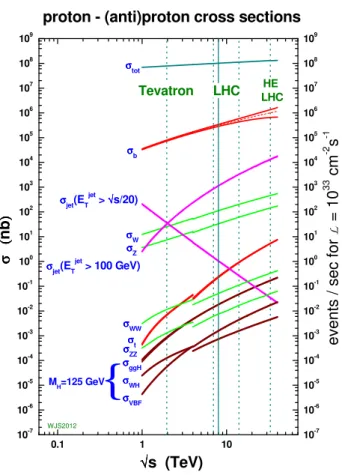
proton - (anti)proton cross sections

σ σ σ σ_W σ σ σ σ_Z σ σ σ σ_t σ σ σ σ (((( n b )))) √ √√ √s (TeV)

{

Figure 1.2: Cross sections for various SM processes as a function of the centre-of-mass energy. From [14].

My main interest on joining ATLAS was its potential to discover new physics phenomena. For various reasons outlined later my personal involvement centers on the searches for the resonant structures in the dielectron final state. At the same time I was exposed to the full spectrum of the ATLAS exotics searches through my work on the ATLAS trigger.

The trigger is crucial in the hadronic-collider environment, as the cross-sections for the pro-cesses of interest are much lower than the total cross-section, as shown in Figure 1.2. With the design LHC collision rates of the order of few tens of MHz it is not possible to record 100% of the collision events. To efficiently reject the high-rate backgrounds online, while maintaining excellent and unbiased efficiency for even the rare signals poses huge challenges to the trigger. How to decide which events to record and which not, making sure that no interesting signals (potentially from the new physics channels, which we have not thought of yet!) are missing, has been my major preoccupation in the last ten years.

Chapter 2 introduces the experimental apparatus: the LHC, the ATLAS detector and basic object reconstruction. Chapter 3 describes the ATLAS trigger and how we decide which data to collect. Chapter 4 describes my quest in search for the new phenomena in the dilepton final state and Chapter 5 outlines some ideas which I would like to explore in the future.

(11)

Chapter 2 Experimental Setup

2.1 The Large Hadron Collider

The Large Hadron Collider (LHC) [15] at the European Organization for Nuclear Research (CERN) is a 27 km circular collider. Its energy reach is limited by its maximum magnetic field (8 T). This magnetic field, used to steer the particles around the ring, is provided by 1232 super-conducting NbTi dipole magnets cooled to a temperature of 1.9 K. The LHC is designed to operate at the proton-proton center-of-mass energies of up to 14 TeV and the nominal luminosity of 1034cm−2 s−1.

The LHC beam parameters, beam sizes and beam intensities are determined by the per-formance of its injector complex. First protons are extracted by ionizing hydrogen atoms and fed into a linear accelerator, Linac-2 which accelerates them to 50 MeV. Then the Booster and the proton synchrotron (PS) are used to prepare the proton bunches and to accelerate them to 25 GeV, the injection momentum of the super proton synchrotron (SPS). Finally the beam is injected from the SPS into the LHC ring at 450 GeV.

The LHC can be operated with different filling schemes which have to meet certain require-ments. There is always a window of at least 119 empty bunches, called abort gap to allow for the beam-dump-kicker rise-time. In total there are 3564 possible bunch positions spaced at 25 ns prepared in the PS. The SPS can provide bunch trains consisting of 72 bunches each and with spacing of 8 bunches corresponding to the SPS-injection-kicker rise-time. Those bunch trains are combined into batches of 3 or 4 with either 38 or 39 bunch spacing to allow for the

LHC-Table 2.1: Evolution of the typical LHC settings at Interaction Points 1 and 5 with time. Year Energy Peak Luminosity Integrated Number of average

Bunch-[TeV] [1033 cm−2 s−1] Luminosity pile-up events spacing [ns]

Design 14 10 - 23 25 2009 0.9/2.36 7×10−7 ∼ 12 − 20µb−1 -2010 7 0.2 48.1 pb−1 2 150 2011 7 3.7 5.46 fb−1 9 50 2012 8 7.7 22.8 fb−1 23 50 2015 13 5.2 4.2 fb−1 14 25 6

(12)

2.2. THE ATLAS DETECTOR OVERVIEW 7

injection-kicker rise-time. Thus the maximal number of bunches which can be put into the LHC is 2808 filled bunches with 25 ns spacing or 1380 with 50 ns spacing.

At the four LHC interaction points the two beams are brought into collision. With more than 1011 protons per LHC bunch at the design luminosity and bunch-spacing there should be on average 23 interactions per bunch-crossing (pile-up).

The LHC started single beam operations in 2008 and achieved first collisions in 2009. Typical LHC operating conditions are summarized in Table 2.1. They can be split into a few distinct periods:

• Run 1 covers lower energy data-taking up to early 2013.

• Run 2 covers data-taking at energies of 13 TeV and above which started in 2015 and will continue till the end of 2018.

• Run 3 (Phase 1) is expected to start in the beginning of 2021. Its main feature should be the LHC luminosity reaching twice its nominal design value (2×1034 cm−2 s−1) inducing 60 interactions per bunch-crossing on average.

• High-Luminosity LHC Run (Phase 2) is expected to start in the end of 2026. Its main feature should be the LHC luminosity increase to 5×1034 cm−2 s−1and about 140 interactions per bunch-crossing on average.

The data-taking periods are interleaved with the long-shutdown periods (LS):

• LS1 (2013-2015) was used for the consolidation of the machine elements to achieve design beam energy and luminosity.

• LS2 (2019-2020) is planned for the upgrade of the injector system.

• During LS3 (2024-2026) the LHC plans major upgrade to its components (installation of the new focusing quadropoles, crab cavities in the interaction regions etc.).

Each LHC improvement (either luminosity or energy increase) offers a major gain in physics potential through increasing sensitivity to higher-mass or lower-cross-section processes. For the LHC detectors those increases in physics potential come with considerable challenges as the increased luminosity brings much higher levels of pile-up events, radiation etc. To exploit maxi-mally the new physics reach and preserve its physics acceptance the ATLAS detector will undergo a series of upgrades as will be discussed later in this manuscript.

2.2 The ATLAS Detector Overview

The ATLAS [16] experiment at the LHC is a multi-purpose particle detector.

Its broad physics program, ranging from precisions SM measurements to searches for the SM Higgs boson and the new physics phenomena, requires precise identification and measurements of charge and momenta over a wide range for electrons, muons, photons, b-jets, tau-leptons and jets, placing stringent requirements on the detector design. The variety of signatures is important in the high-rate environment of the LHC in order to achieve robust and redundant physics mea-surements with the posibility of internal cross-check. Large acceptance in pseudorapidity with

(13)

8 CHAPTER 2. EXPERIMENTAL SETUP

Figure 2.1: The ATLAS detector. [16]

almost full azimuthal-angle coverage is crucial for the missing transverse energy measurements, providing sensitivity to any particles which do not interact in the detector.

Due to the experimental conditions of the LHC, every candidate event is accompanied by other inelastic events in the same bunch crossing, averaging 23 events at the nominal luminosity. This overlap of pile-up events can be reduced by using highly granular detectors with good time resolution, giving low occupancy at the expense of having a large number of detector channels. High particle fluxes emanating from the interaction region lead to high radiation levels, requiring radiation-hard sensors and electronics.

The overall ATLAS detector layout is shown in Figure 2.1. It has a cylindrical geometry1 covering almost the entire solid angle around the interaction point. The detector components are described as barrel if they are in the central region of pseudorapidity or endcap if they are in the forward regions.

Starting from the interaction point, the Inner Tracking Detector (ID) consists of a three layer silicon pixel detector in the barrel (three disks in the endcaps), microstrip detector called SemiConductor Tracker, (SCT) with the four-layers in the barrel (9 disks in the endcaps) and straw-tube tracking detector with transition radiation capability (Transition Radiation Tracker, TRT) surrounding it. For Run 2, a new pixel layer (Insertable B-layer, IBL) has been added at 1_{ATLAS uses a right-handed coordinate system with its origin at the nominal interaction point (IP) in the}

center of the detector and the z-axis along the beam pipe. The x-axis points from the IP to the center of the LHC ring, and the y-axis points upward. Cylindrical coordinates (r, φ) are used in the transverse plane, φ being the azimuthal angle around the z-axis. The pseudorapidity is defined in terms of the polar angle θ as η = − ln tan(θ/2).

(14)

2.3. OBJECT RECONSTRUCTION 9

a radius of 3.3 cm. Both the Pixel and SCT cover the region |η| < 2.5, while the TRT covers |η| < 2.0. The magnetic field for the inner tracking is provided by a thin superconducting solenoid generating field of 2 T.

The electromagnetic (EM) calorimeter is a lead-liquid argon (LAr) sampling calorimeter with an accordion geometry, divided into a barrel section covering the region |η| <1.45 and two endcap sections (EMEC) covering the region 1.375 < |η| < 3.2. The EM calorimeter has three longitudinal layers:

• The first layer has a thickness of 3−5 radiation length and a high granularity in η, providing discrimination between single photons and photon pairs from π0 decays in jets.

• The second layer collects most of the EM shower energy and has thickness of about 17 radiation length and a granularity0.025 × 0.025 in η × φ.

• The third layer collects the tail of the shower and has a coarser segmentation, allowing to discriminate between electrons and hadrons (e.g. π±).

The central EM calorimeter has a thin pre-sampler layer at |η| < 1.8 to correct for upstream energy losses. In the endcap LAr technology is used for the hadronic calorimeter. The forward regions are instrumented with LAr calorimeters for both EM and hadronic energy measurements up to |η|= 4.9. Those detectors are housed in one barrel and two endcap cryostats. The barrel of the hadronic calorimetry (|η| <1.7) is provided by an iron-scintillator tile sampling calorimeter using wavelength-shifting fibers.

The calorimetry is surrounded by the muon spectrometer (MS) mounted in and around air core toroids that generate an average field of 0.5 T in the barrel and 1 T in the endcap regions. Precision tracking information is provided by three stations of Monitoring Drift Tubers (MDT) in the region |η| < 2.7 (2.0 for the innermost layer) and by Cathode Strip Chambers (CSC) in the region 2.0 < |η| < 2.7. First level trigger uses information from the Resistive Plate Chambers (RPC) in the barrel (|η| <1.05) and the Thin Gap Chambers (TGC) in the endcaps (1.05 < |η| < 2.4).

The online event selection must reduce the billion interactions per second to a few hundred events per second for storage, without any loss of interesting physics events. The ATLAS trigger system consists of two main levels: a hardware based Level 1 (L1) and a software-based High-Level-Trigger (HLT). It is described in detail in the next chapter.

The detector has operated with efficiencies exceeding 99.6% per subsystem in the 2012 run (95.5% of events all good for physics) and with performance characteristics very close to its design values.

2.3 Object Reconstruction

This section briefly discusses objects used in dilepton physics analysis: electrons and muons.

2.3.1 Electrons

Only electrons within the inner-detector acceptance (e.g. |η| < 2.47) are considered in this manuscript. More detailed overview of electron reconstruction, identification and calibration can be found in Refs. [17,18,19].

(15)

Energy reconstruction in the LAr calorimeter

Figure 2.2: The current LAr readout electronics architecture from Ref. [20].

Charged particles from EM shower ionize the liquid argon in the calorimeter. Under the influence of the electric field, the ionization electrons drift towards the electrode inducing a current, which is proportional to the energy deposited in the liquid argon.

The current LAr readout electronics architecture is shown in Figure 2.2. As one can see there are two separate read-out paths: one with coarse granularity (Trigger Towers) used for the first-level of the trigger and one with fine granularity used by the high-level-trigger and offline reconstruction. The description below concentrates on the latter.

Inside a front-end-board (FEB), the signal is first pre-amplified. Then shaper splits output signal into three overlapping linear gains: high (gain ratio=82), medium (gain ratio=8.4), and low (gain ratio=0.8) to cover energies ranging from a few TeV down to the noise level. Figure2.3

shows a typical triangular pulse shape of the ionization signal along with the shaped and sampled signal shape. The output shaped signal is sampled at 40 MHz and, for events selected by the L1 trigger, five2 samples around the peak spaced by 25 ns are extracted and sent to a 12-bit

2

(16)

2.3. OBJECT RECONSTRUCTION 11

Figure 2.3: The amplitude vs. time for the triangular pulse shape from the LAr calorimeter, overlaid with the bipolar-shaped and sampled pulse shape (from Ref. [20]).

analog-to-digital converter (ADC).

The Readout Driver (ROD) modules receive raw data from the FEBs and use the Optimal Filtering method to calculate the amplitude of the pulse (A, ADC counts) and the difference between digitization time and the chosen phase (∆t, ns):

A= n X i=0 ai(si− p), (2.1) ∆t = 1 A n X i=0 bi(si− p), (2.2)

where ai and bi are the Optimal Filtering Coefficients (OFCs) computed per cell from the

pre-dicted ionization pulse shape and the measured noise autocorrelation to minimize the noise and pile-up contributions, s_iare the samples, p is the electronic pedestal and n represents the number of samples used.

Note that if the samples are shifted in time, this leads to wrong computation of OFCs. For example, a time shift corresponding to ∼ 5 ns leads a 0.5% bias on the energy reconstruction. Precise measurement of the time of the signal peak is also a valuable input for exotic particle searches with a long lifetime or for very massive stable particles. The timing can be influenced by various factors (the length variation of the optical fibers delivering the LHC clock to the ATLAS experiment due to temperature change, wrong calorimeter high-voltage module settings, FEB internal delays, different cable length for each FEB etc.). Some of those factors are constant and were corrected for in the beginning of data-taking, but others could change with time and thus have to be monitored constantly. The timing alignment of the LAr calorimeter cells was better than 1 ns in 2011 [21] and better than 500 ps [22] in 2012.

The stability of the electronic response of the readout cells (i.e. pedestal, noise and gain) is regularly monitored using dedicated calibration runs. The pedestal and noise for each cell are

(17)

computed in the dedicated daily Pedestal calibration runs as the mean of the signal samples siin

ADC counts and the width of the energy distribution, respectively. The same runs also provides information on the noise auto-correlation needed for the OFC coefficient calculation. In so-called Ramp and Delay calibration runs, calibrated current pulses are injected through high-precision resistors to simulate energy deposits in the calorimeters and the corresponding cell responses are reconstructed. Ramp runs are used to measure the gain (G) as well as the factor F_DAC→µA which converts digital-to-analog converter (DAC) counts set on the calibration board to µA. The weekly Delay runs measure the full calibration pulse shapes. The results of those calibration runs are analyzed and if any differences with respect to reference values are observed the online database is updated so that correct values can be used for the energy calculation.

Including the relevant electronic calibration constants, the deposited energy (in MeV) is determined as:

Ecell= FµA→ MeV× FDAC→µA×

1

Mphys

Mcali

× G × A, (2.3)

where the factor _Mphys1 Mcali

quantifies the ratio of response to a calibration pulse and an ioniza-tion pulse corresponding to the same input current and the factor FµA→ MeV is estimated from

simulations and beam test results.

Offline Electron Reconstruction and identification

Electron reconstruction starts with a creation of an EM cluster using a sliding-window algorithm with size of3 × 5 cells in (η, φ) space in the middle calorimeter layer from energy deposits with total E_T>2.5 GeV. Tracks reconstructed in the inner detector with pT>0.5 GeV are extrapolated

to the calorimeter and matched to the EM cluster. An electron is considered to be reconstructed if at least one track is matched to the cluster. Matched clusters are then rebuilt with a slightly larger window, 3 × 7 in the barrel or 5 × 5 in the endcap.

In Run 1 a cut-based selection was used for the electron identification. It has sequential cuts optimized in cluster-η×E_T bins on calorimeter shower-shapes, tracking, track-cluster matching and TRT-identification variables. For the list of the selection variables please see Ref. [17]. The selection exploits the fact that the shower development is narrower and shorter for electrons than for hadrons. There are at least three nested sets of selection criteria, labeled loose, medium and tight with increasing background-rejection power obtained by adding discriminating variables at each step and by tightening the selection on the initial variables.

The electron selection evolved with time. For example in 2009-2010 electron selection at all levels tended to be rather loose focusing on robustness as the detector was still undergoing commissioning with the first LHC data. For 2011, electron selection needed to be tightened considerably to increase background rejection power in the much higher pile-up conditions and minimize its pile-up dependence. For more details on the 2011 configuration see Ref. [19]. In 2012, electron tracking was improved offline [23] with the introduction of the Gaussian Sum Filter algorithm which accounts for the non-linear bremsstrahlung effects. Electron selection had to be re-tuned again to remove the residual pile-up dependences.

For Run 2 electron identification moved from the more robust cut-based to more performant likelihood-based identification criteria maintaining the same selection variables. Generally the likelihood-based selection provides about a factor two improvement in background rejection for the same signal efficiency with respect to the optimized cut-based electron selection.

(18)

2.4. MY CONTRIBUTIONS 13

The electron four-momentum is built from the cluster energy and the direction of the asso-ciated track from the ID. The final cluster energy is obtained by correcting for the energy losses in the material in front of the calorimeter, the lateral leakage due to the fixed cluster size and the longitudinal leakage to the hadronic calorimeter.

2.3.2 Muons

This information is provided for completeness. I have not performed any work on the muon reconstruction, but muons were used in the analysis presented later. More detailed overview of muon reconstruction and identification can be found in Ref. [24].

In Run 1 several types of algorithms for reconstructing muons were available in ATLAS. Most analysis use so-called combined muons: track reconstruction is performed independently in the ID and MS, and a combined track is formed from the successful combination.

There are various ways to do this combination, for example one can perform a statistical com-bination of the track parameters of the stand-alone and the ID muon tracks using corresponding covariance matrices (Chain 1). One can also perform a global refit of the muon track using hits from both the ID and MS sub-detectors (Chain 2). The use of two independent codes provided redundancy during commissioning phase, but caused problems as there there was non-negligible non-overlap between the reconstructed muon candidates as discussed in Section 4.3. A unified reconstruction program has been developed in 2012 to be used for the future data-taking.

In addition to the standard muon selection, requiring a minimum number of hits in each of the ID components etc. exotics searches with high-pT muons applied a special high-pT muon

selection detailed in Ref. [25]. Muon momentum is taken from combined fit.

2.4 My contributions

• In 2008-2010 I was responsible for the documentation of the ATLAS electron and pho-ton performance group summarizing object reconstruction, selection variables, calibration procedures, etc. on the web and in the code (doxygen).

• In 2011 I was a member of the LAr electronics calibration team responsible for the validation of the calibration runs.

• In 2009-2011 I supervised Ludovica Aperio-Bella’s work on the LAr timing alignment [21]. She developed the LAr cells timing methodology and achieved the global LAr timing align-ment below the one ns for all the LAr partitions, and the EM barrel time resolution below the 1 ns level.

(19)

Chapter 3 ATLAS Trigger and Trigger Menu

This chapter discusses ATLAS trigger developments over the past ten years. This overview concentrates on the aspects I worked on. Its focus varies with the evolution of my responsibilities within the trigger group.

3.1 Introduction

Nominal LHC bunch-spacing is 25 ns. This means that every 25 ns there could be a potentially interesting event which needs to be recorded. Each event has a size of ∼1 Mb - thus it is not possible to store 100% of the events. The multi-level trigger system reduces the 40 MHz sampling rate to a few hundred Hz of events for offline reconstruction and physics analysis. Each trigger level refines the decisions made at the previous level and, where necessary, applies additional selection criteria. Each trigger level has its own constraints (timing, output rate1, etc.) which change during the lifetime of the experiment, as summarized in Table3.1, to preserve the physics acceptance despite the LHC luminosity increases.

Stable operation of the trigger is crucial as many parts of the system constitute a single point of failure, with problems potentially leading to loss of physics data. Detailed monitoring and thorough testing of any modifications are essential to ensure the smooth data-taking.

1

Note that while usually the peak rate provides main constraint for the trigger, for the last level of the trigger the main constraint comes from the average output rate. In a fill with a certain peak luminosity, trigger rates follow the luminosity decrease with time. In general it was noted that the average luminosity in a typical run is about 2/3 of the peak luminosity. Thus peak rate = 1.5× average rate.

Table 3.1: Trigger Rate Evolution. Maximum L1 accept rate which the detector readout systems can handle in Run 1 was 75 kHz, upgradable to 100 kHz. High Level Trigger (HLT) in Run 1 consisted of two separate levels: Level 2 (L2) and Event Filter (EF).

Design Run 1 Run 2 peak L1 Rate (kHz) 75(100) 65 90 peak L2 Rate (kHz) 3.0 5.5 -average HLT (EF) Rate (Hz) 200 400 1000

(20)

3.2. ATLAS TRIGGER OVERVIEW 15

The trigger system is configured via the trigger menu. The trigger menu specifies which event selection algorithms are enabled and thus it is of critical importance for the physics program of ATLAS. The menu should provide efficient coverage to all physics processes of interest from the SM measurements to the searches for physics beyond the SM, including everything we have not yet thought of. If a physics signal does not have a trigger matched to its signature, it would not be possible to do the corresponding analysis or the analysis would have suboptimal sensitivity.

The trigger menu is designed to have the best possible physics sensitivity at a given luminosity while keeping trigger rates, CPU consumption etc. within the resource limitations of the trigger and data acquisition system (DAQ). In order to provide a coherent dataset for physics analyses, the trigger menu has to be as stable as possible.

To address those somewhat conflicting requirements and decide on the final configuration of the trigger menu, the ATLAS Collaboration has a dedicated Menu Coordination Group (MCG). It is led by Trigger Menu Coordinators and consists of ATLAS management, physics, data-preparation and run coordinators, trigger management as well as representatives from all the combined performance and physics analysis groups (about 20-30 people in total). Most of my trigger activities described in this manuscript have been performed as a member of this group.

The rest of this chapter is constructed as follows: a general overview of the ATLAS trigger (Section 3.2) is followed by the description of the trigger system in Run 1 (Section 3.3) and the Run-1 menu development time-line (Sections 3.4-3.5). Section 3.6describes updates of the trigger system for the Run 2. Section 3.7 reviews the Run 2 trigger menu and the last two sections provide conclusions and summarize my contributions in the domain of the trigger.

3.2 ATLAS Trigger Overview

3.2.1 First Level Trigger

The first level trigger (L1) is based on fast, custom electronics using low-granularity signals from the calorimeters (L1Calo) and fast signals from dedicated muon trigger chambers (L1Muon). The main available L1 trigger signatures and their maximum number of the L1 thresholds are shown in Table3.2.

L1 Calorimeter Trigger

The L1Calo trigger is based on inputs from the electromagnetic and hadronic calorimeters cover-ing region |η| <4.9. It provides triggers for signals consistent with a high transverse momentum electron/photon, tau and jet or large missing transverse energy (E_Tmiss). The L1Calo trigger threshold2 is applied to a transverse energy (ET).

L1 Muon Trigger

The L1 muon trigger system identifies muons by the spatial and temporal coincidence of RPC and TGC hits. The degree of deviation from the hit pattern expected for a muon with infinite momentum is used to estimate the p_T of the muon at six possible thresholds. The L1 triggers generated by hits in the RPC require a coincidence of hits in the three layers for the highest three 2 _{It is possible for the calorimeter threshold to be pseudorapidity dependent to take into account the energy}

(21)

16 CHAPTER 3. ATLAS TRIGGER AND TRIGGER MENU

Table 3.2: The key trigger objects identified by the trigger system, their shortened representation used in the trigger menus and the number of the L1 thresholds available for each of the object types.

Representation Number of L1 Thresholds

Trigger signature L1 HLT Design Run 1 Run 2

electron EM e 8 9 16

photon EM g as above as above as above

muon MU mu 6 6 6

jet J j 12 12 25

tau TAU tau 8 7 16

E_Tmiss XE xe 8 8 8

E_Tmiss(|η| < XX) XE.0ETAXX xe.0etaXX - - 8

PET TE te 4 4 8

PE_T(|η| < XX) TE.0ETAXX te.0etaXX - - 8

total jet energy JE je 4 4

-E_Tmisssignificance XS xs - 8 8

b-jet - b - -

-pT thresholds, and a coincidence of hits in two of the three layers for the other three thresholds.

The L1 triggers generated by hits in the TGC require a coincidence of hits in the three layers, except for limited areas in the lowest threshold.

Central Trigger Processor

The information from L1Calo and L1Muon systems is sent to the Central Trigger Processor (CTP), where it is combined and the result is compared to the pre-programmed L1 trigger items. The maximum allowed number of the L1 trigger items (256 in Run 1 and 512 in Run 2) as well as their possible AND/OR combinations are fixed by the CTP hardware. If the trigger conditions are met, a L1 Accept is issued initiating the detector readout. The maximum L1 accept rate is limited by the detector readout system to be about 75 kHz in Run 1, upgradable to 100 kHz. The L1 trigger decision must reach the front-end electronics within 2.5 µs after the bunch crossing it is associated with.

3.2.2 High Level Trigger and Trigger Menu Overview

The High Level Trigger (HLT) is software-based and runs on large PC-farms. The HLT receives the L1 trigger decision together with information on so-called Regions-of-Interest (RoIs) around the L1 objects. The RoI information is used to perform regional event reconstruction. In addition, the full detector event data is available to the HLT as needed. HLT has a few seconds to decide if an event should be kept or not and its average output rate is limited by the offline computing resources available for the data storage and processing.

A trigger selection is organized into so-called trigger chains, each consisting of one specific L1 selection seeding a sequence of selection algorithms in the HLT. Each chain is responsible for selecting a specific physics signature. An example of a single electron trigger chain is discussed

(22)

3.2. ATLAS TRIGGER OVERVIEW 17

in Section3.4.1.

Further flexibility is provided by defining bunch groups, which allow trigger chains to include specific requirements on the LHC bunches colliding in ATLAS. These requirements include paired (colliding) bunch-crossings for physics triggers, empty or unpaired crossings for background stud-ies and dedicated bunch groups for detector calibration.

A full selection of the trigger chain is encoded in its trigger name which consists of the trigger level, multiplicity, particle type (specified in Table 3.2) and p_T-threshold value in GeV (e.g. L1_2MU4, HLT_mu40). The L1 objects are written in capital letters and a trigger name without level prefix refers to the entire trigger chain. Further selection criteria (tightness or type of identification, isolation, reconstruction algorithms, etc.) applied to a given trigger object at the HLT are appended to the trigger name (e.g. g120_loose is a 120 GeV photon trigger with a loose selection applied to photon objects). In case of ambiguity, the L1 seed is also suffixed to the trigger name (e.g. e24_lhmedium_L1EM20VH). Triggers executed without a requirement on the L1 seed have “noL1” attached to their pT-threshold value.

There are four different classes of trigger chains:

• Single-object triggers: used for final states with at least one characteristic object.

• Multi-object triggers: used for final states with two or more characteristic objects of the same type.

• Combined triggers: used for final states with two or more characteristic objects of different types. For example, a 60 GeV photon plus 60 GeV E_Tmiss trigger with no L1 Emiss_T require-ment would be denoted g60_loose_xe60noL1.

• Topological triggers: used for final states that require selections based on information from two or more RoIs. For example the mu6_j150_dr05 trigger for b-jet calibration studies requires a 150 GeV jet and a 6 GeV muon to be within |∆R| < 0.5 of each other.

The full set of trigger chains is called the trigger menu. A typical menu contains around one thousand chains. It includes not only a few hundred primary physics chains, but also a large set of support triggers to allow background and efficiency measurements as well as monitoring and calibration triggers which collect data to ensure the correct operation of the trigger and detector. Prescale factors can be applied to each L1 and HLT trigger, such that on average only 1 in N events passing the trigger causes an event to be accepted at that trigger level. Prescales can also be set so as to disable specific chains. Prescale values can be changed during data-taking to ensure the optimal trigger menu for a given LHC luminosity. Trigger menu prescale sets determine the exact menu configuration which is run online.

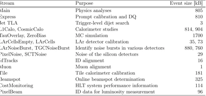
Data for events selected by the trigger system are written to inclusive data streams3. Table3.3

provides a list of main streams and their typical event size. Physics streams contain information from the whole detector. About 10-20 Hz of those physics events are also written to an express stream where prompt offline reconstruction provides calibration and Data Quality information prior to the reconstruction of the other physics streams. There are about a dozen additional streams for calibration, monitoring and detector performance purposes. Some of these streams use partial event building to record only the relevant sub-detector data, thus decreasing the event size significantly. Any events for which the trigger is unable to make a decision because of the

3

(23)

Table 3.3: Trigger streams and their average (compressed) event size per event in 2015.

Stream Purpose Event size [kB]

Main Physics analyses 805

Express Prompt calibration and DQ 810

Jet TLA Trigger-level dijet search 3

L1Calo, CosmicCalo Calorimeter studies 814, 904

TauOverlay, ZeroBias MC simulation 1700

LArCellsEmpty, LArCells LAr detector calibration 35, 73 LArNoiseBurst, TGCNoiseBurst Identify noise bursts in various detectors 880, 760 PixelNoise, SCTNoise Noise of the silicon detectors 29

IdTracks ID alignment 16

Muon Muon alignment 1

Tile Tile calorimeter calibration 181

Beamspot Online beamspot determination 325

CostMonitoring HLT system performance information 114

PixelBeam ID data for luminosity measurement 96

trigger time-out or any other failure in the online software, are recorded to a special stream called debug stream. Those events can be later re-analyzed offline.

3.3 Prehistory: ATLAS Trigger System in Run 1 and “Design”

Trigger Menu

Figure 3.1: Overview of the ATLAS trigger and DAQ system in 2012 [26].

(24)

3.3. PREHISTORY: ATLAS TRIGGER SYSTEM IN RUN 1 AND “DESIGN” TRIGGER MENU 19

unchanged for the whole Run 1. As shown in the figure, the original design assumed a three-level system with a hardware-based L1 followed by an HLT consisting of two software-based levels: Level-2 (L2) and Event Filter (EF). L1 reduced the 40 MHz sampling rate to 75 kHz in 2 µs. In Run 1 L2 was running customized fast algorithms and requesting the data for the relevant detectors based on the RoIs defined by the L1. It had to make a decision in about 40 ms and reduced rate to about 2-5 kHz. The EF reduced rate to 200 Hz in about 4 seconds and used offline reconstruction algorithms adapted for the trigger in order to achieve the best performance on the full event data.

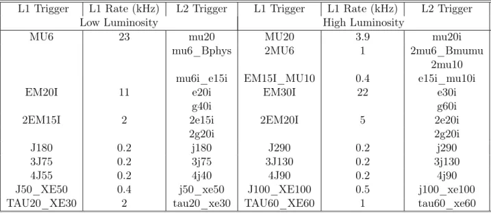
Table 3.4: Original L1 and L2 low and high luminosity menu for center-of-mass energy of 14 TeV. Note that this menu uses special naming convention. The calorimeter threshold values correspond to the point where L1 (L2) algorithms are 95%(90%) efficient. For the Emiss

T trigger the threshold

value corresponds to the cut. The muon thresholds correspond to a point of 90% efficiency at L1, not accounting for inefficiency due to the limited detector coverage.

L1 Trigger L1 Rate (kHz) L2 Trigger L1 Trigger L1 Rate (kHz) L2 Trigger

Low Luminosity High Luminosity

MU6 23 mu20 MU20 3.9 mu20i

mu6_Bphys 2MU6 1 2mu6_Bmumu

2mu10 mu6i_e15i EM15I_MU10 0.4 e15i_mu10i

EM20I 11 e20i EM30I 22 e30i

g40i g60i

2EM15I 2 2e15i 2EM20I 5 2e20i

2g20i 2g20i

J180 0.2 j180 J290 0.2 j290

3J75 0.2 3j75 3J130 0.2 3j130

4J55 0.2 4j40 4J90 0.2 4j90

J50_XE50 0.4 j50_xe50 J100_XE100 0.5 j100_xe100

TAU20_XE30 2 tau20_xe30 TAU60_XE60 1 tau60_xe60

The first set of ATLAS trigger menus appeared in 1998 [27] and was refined in 1999 [28]. These menus shown in Table 3.4 addressed two scenarios: low luminosity (1033 cm−2 s−1) and high luminosity (1034cm−2s−1) at√s= 14 TeV aiming at about 40 kHz at L1 and about 2000 Hz at L2.

It can be noted that even this rather limited set of triggers covers a significant portion of the physics goals of the ATLAS experiment. In particular the inclusive lepton and dilepton triggers provide W → lν and Z → ll selections, where l designates electron or muon, giving unbiased triggers for many SM and BSM searches which have those gauge bosons in their final state as well as covering other multi-lepton final states.

The diphoton trigger (2g20i) is targeting the very important H → γγ channel and would be useful for searches for HH → bbγγ or other Higgs-boson-like final states as well as the BSM searches with two or more photons. The inclusive photon trigger proposals are mostly targeting BSM physics with photon thresholds being quite high.

(25)

Searches without leptons in the final state (including supersymmetry searches with or with-out E_Tmiss) were supposed to be covered by the jet triggers, which had very optimistically low thresholds.

There are only two more special-purpose trigger “lines” in this menu: τ+Emiss

T triggers for

the W → τ ν final state (although this would also serve for some supersymmetry searches) and B-physics triggers, which are low pTdimuon triggers with invariant mass or common vertex cuts.

This menu follows the main principle behind the ATLAS trigger menu strategy in the years to come: to keep triggers as general as possible to cover the widest possible range of physics signatures. It is the most long-living ATLAS trigger menu proposal which had survived in its original form for 10 years unchallenged.

3.4 Antiquity: Pre-data-taking ATLAS Trigger Menu

3.4.1 Online electron reconstruction

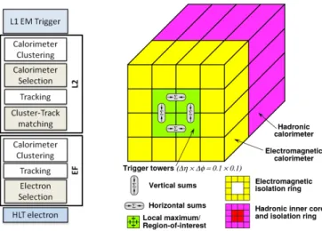
Figure 3.2: (right)Typical Run 1 electron trigger chain. (left) Building blocks of the elec-tron/photon and tau algorithms with the sums to be compared to programmable thresholds. From [29].

One of my first tasks in 2006 when I joined the ATLAS experiment was to optimize the electron trigger selection to minimize an efficiency loss with respect to the offline selection. A typical Run 1 electron trigger chain is shown in Figure3.2(left).

First the electromagnetic cluster reconstruction at L1 identifies a Region of Interest as a 2 × 2 trigger tower cluster in the EM calorimeter for which the ET-sum from at least one of

the four possible pairs of nearest neighbor towers exceeds a pre-defined threshold as shown in Figure3.2 (right). Isolation-veto thresholds can be set for the 12-tower surrounding ring in the EM calorimeter (denoted by “I”), as well as hadronic tower sums in a central 2 × 2 core behind the cluster (hadronic veto, denoted by “H”). The threshold could be set with 1 GeV precision and with∆η =0.4 granularity.

Seeded by the position of the L1 cluster, the L2 electron selection employs fast calorime-ter reconstruction algorithm followed by fast tracking reconstruction. Then, at the EF, further

(26)

3.4. ANTIQUITY: PRE-DATA-TAKING ATLAS TRIGGER MENU 21

calorimeter cluster and track reconstruction is performed but using the offline precision recon-struction algorithms. Due to timing constraints the HLT reconrecon-struction algorithms (especially the fast tracking) are less refined than the corresponding offline algorithms leading to potential inefficiencies.

After investigating the sources of efficiency loss it became clear that the leading one was due to differences in variables or cuts between the online and offline selections. Ensuring that the selection at EF was the same or looser than the offline one allowed to increase electron trigger efficiency by approximately 3%.

3.4.2 Development of electron triggers for the low-pT region

Figure 3.3: A sketch of known and hypothetical potential sources of electrons (e) at the LHC experiments: grey corresponds to J/ψ → ee decays, open histogram to Υ, blue to b, c → e, red to W , magenta to Z, green to Drell-Yan (mee <60 GeV), cyan (enhansed by a factor of 1000)

to 1 TeV Z0.

In early 2007, as data-taking approached a concern was raised about the absence of a trigger menu strategy for the LHC luminosities lower than 1033 cm−2 s−1. With the unknown LHC start-up schedule, it was not clear how fast we would accumulate sufficient statistics of Z → ee events for electromagnetic calorimeter commissioning, electron performance studies, etc.

By studying potential sources of electrons, shown of Figure 3.3, it became clear that there should be significant statistics of electrons coming from J/ψ → ee andΥ → ee decays. Assuming dielectrons with pT>3 GeV, cross-sections of pp → Z : J/ψ : Υ → ee are expected to scale as

2:120:50. Unfortunately as shown in Figure3.4, most of the signal events are centered at very low electron p_T. It is very challenging to trigger on these events at L1, as the L1 calorimeter trigger performance at low-energies is limited by the noise of about 0.5 GeV per RoI. A 3 GeV threshold (EM3) was assumed to be the lowest limit of what is feasible for the L1Calo. The L1 rate studies showed that typical rate of 2EM3 trigger is expected to be 650 kHz at 1033 cm−2 s−1 (√s = 14 TeV) which is much higher than maximal L1 bandwidth. But for lower luminosity points,

(27)

22 CHAPTER 3. ATLAS TRIGGER AND TRIGGER MENU /MeV T p high e 0 1 2 3 4 5 6 7 8 9 10 3 10 × /MeV _T p low e 0 1 2 3 4 5 6 7 8 9 10 3 10 ATLAS /MeV T p high e 0 1 2 3 4 5 6 7 8 9 10 3 10 × /MeV_T p low e 0 1 2 3 4 5 6 7 8 9 10 3 10 ATLAS

Figure 3.4: Distribution of the generator-level transverse momentum of the less energetic electron versus the transverse momentum of the most energetic electron in the direct J/ψ (left) and Υ (right) decays.

such as 1031_cm−2 _s−1_{, L1 output rate becomes only 6.5 kHz, which although taking a significant}

fraction of the total L1 bandwidth, is potentially feasible.

The proposed strategy to trigger on J/ψ and Υ → ee events was based on two low-ET L1

electromagnetic RoIs and further electron identification using calorimeter and inner-detector information at the HLT. At a luminosity of 1031 cm−2 s−1 this trigger can run unprescaled, which would allow ATLAS to collect about 100k events with J/ψ and 30k with Υ decays in 100 pb−1 of data respectively. In the same sample one would expect to collect about 30k of Z → ee events.

Currently the J/ψ triggers are an essential part of the ATLAS trigger menu even though they are usually prescaled for luminosities above 1031 cm−2 s−1. One of the electron candidate selections is loosened with respect to the original proposal to enable tag-and-probe studies. It is also not a single trigger but a set of triggers with pT-requirements and tightness of identification

criteria varying between the two electrons. The combination of triggers was introduced to allow more uniform event collection as a function of p_T as well as enabling tag-and-probe studies. These triggers provide a unique event sample for electron performance studies in the range 7 − 20 GeV [17], complementing electrons from Z decays which cover the range above 15 GeV. This region of the electron p_T is crucial for analyses with multi-lepton final states in general and, in particular, for the observation of the Higgs boson in the H → ZZ →4l channel [10].

3.4.3 2008 trigger menu proposal

In 2008 I was nominated as trigger menu liaison for the electron and photon performance group. My role was to ensure that all the relevant electron and photon triggers needed for performance studies (as well as physics analysis upstream) were present in the ATLAS trigger menu. The J/ψ triggers were one of the main motivations for the creation in 2008 of the 1031 cm−2 s−1 menu shown in Table 3.5. This menu aimed at luminosities a few orders of magnitude below the

(28)

3.5. MIDDLE AGES: ATLAS TRIGGER MENU 2009 - 2012 23

Table 3.5: Draft of Trigger menu for center-of-mass energy of 14 TeV and 1031 cm−2 s−1 from Ref. [16]

Signature L1 Rate (Hz) HLT Rate (Hz) Comments Minimum bias Up to 10000 10 Pre-scaled trigger item

e10 5000 21 b, c → e, W , Z, Drell-Yan, t¯t

2e5 6500 6 Drell-Yan, J/φ, Υ, Z

g20 370 6 Direct photons, γ-jet balance

2g15 100 <1 photon pairs

mu10 360 19 W , Z, t¯t

2mu4 70 3 B-physics, Drell-Yan, J/φ, Υ, Z

mu4+J/ψ(µµ) 1800 <1 B-physics

j120 9 9 QCD and other high-p_T jet final states

4j23 8 5 Multi-jet final states

tau20i_xe30 5000 10 W , t¯t

tau20i_e10 130 1 Z → τ τ

tau20i_µ6 20 3 Z → τ τ

nominal one and thus allowed for very low-threshold single and di-object unprescaled electron, muon and photon triggers compared to the menu proposal in Table 3.4. This menu introduced hadronic single and ditau triggers to target events from Higgs, W and Z bosons important for SM precision measurements as well as beyond SM processes. Although not mentioned explicitly this menu also included b-jet and missing transverse energy triggers for tt measurements and searches of supersymmetry or other exotics particles.

3.5 Middle Ages: ATLAS Trigger Menu 2009 - 2012

3.5.1 Dark Ages: ATLAS Trigger Menu 2009-2010

Figure 3.5: Evolution of the L1 trigger rate throughout 2010 (lower panel), compared to the instantaneous luminosity evolution (upper panel) from Ref. [29].

(29)

Table 3.6: Examples of p_T thresholds and selections for the lowest unprescaled triggers in the 2010 physics menu at center-of-mass energy of 7 TeV from Ref. [29]

Luminosity [cm−2s−1] 3×1030 2×1031 2×1032

Signature pT threshold [GeV], selection

Single muon 4 10 13,tight

Dimuon 4 6 6,loose

Single electron 10, medium 15, medium 15, medium

Dielectron 3, loose 5, medium 10, loose

Single photon 15, loose 30, loose 40, loose

Diphoton 5, loose 15, loose 15, loose

Single tau 20, loose 50, loose 84, loose

Single jet 30 75, loose 95, loose

E_Tmiss 25, tight 30, loose 40, loose

B-physics mu4_DiMu mu4_DiMu 2mu4_DiMu

The LHC circulated first beams in 2008 and achieved first collisions in the end of 2009. In 2009 the peak luminosities did not exceed 7×1026cm−2s−1 and center-of-mass energies were 0.9 TeV and 2.36 TeV which corresponds to a few tens of Hz of the trigger rate. The ATLAS trigger could record the full proton-proton collision event rate without any rejection required. The LHC increased its center-of mass energy to 7 TeV in 2010. The luminosity ramp-up was very slow up to the end of that year: increasing from 1027cm−2s−1 in April 2010, to 1030cm−2s−1 in June 2010, 1031cm−2s−1 in August 2010 and finally reaching 2×1032cm−2s−1 in October 2010 as shown in Figure3.5.

This slow luminosity increase allowed time for thorough trigger commissioning as summarized in Ref. [29]. Only when the peak luminosity delivered by the LHC reached 1.2×1029cm−2s−1, it was necessary to start enabling HLT rejection for the highest rate L1 triggers.

2010 physics trigger menu designed for 1030 _{− 10}32_cm−2_s−1 _{is shown in Table} _3.6_{. The}

bandwidth allocation between different trigger signatures was driven by their importance for the ATLAS physics program. For example electron/photon and muon triggers were assigned 25% of the bandwidth each while b-jet, B-physics, jets, Emiss

T and τ triggers had 5-10% of the

bandwidth each. This menu was deployed online in the end of 2010. To keep trigger rates within the required constraints one had to either raise pT thresholds or tighten the trigger selection.

This ever-changing menu brought unnecessary complication for physics analyses, and the trigger menus for the following years were designed to change as little as possible.

As all these peak luminosity values were at least an order of magnitude below the nominal low luminosity of LHC (1033cm−2 s−1), the considerations behind the 2008 menu proposal (e.g. menu dominated by the low-p_T triggers with loosest selection possible) were very relevant to the ATLAS trigger menu strategy up to the end of 2010. Note that as the 2010 LHC run had a center-of-mass energy of 7 TeV (e.g. half of the nominal value of 14 TeV), trigger rates where roughly a factor of two less than the nominal ones which were considered in Table 3.4 and Table3.5.

(30)

High-pT objects in trigger

In the early 2010 I was appointed to coordinate trigger requests for the ATLAS Exotic analy-ses. The ATLAS Exotics Working Group is studying a wide variety of signatures to discover non-supersymmetric physics beyond the Standard Model. The group covers a wide variety of models, from Extra Dimensions and mini Black Holes to Dark Matter, exotics Higgs modes, Compositeness, etc. Given the wide scope of the physics signatures, the Exotics group takes interest in nearly all types of triggers in the menu, except the Emiss_T triggers which fall into the domain of the supersymmetry working group.

Considering the low thresholds and loose selections of the 2009-2010 ATLAS trigger menu, no dedicated exotics triggers were required. With major effort going into commissioning of the various systems, of particular importance to the Exotics group was ensuring good performance of the triggers for the very-high pT objects, for which it is the main user.

First, the Exotics group wanted to ensure that no events are lost at L1, in particular for the calorimeter triggers. The extensive preparation work described below was done by the L1Calo experts. In order to assign the calorimeter tower signals to correct bunch-crossing, the signals must be synchronized to the LHC-clock phase with nanosecond precision. This was done with calorimeter pulser systems and cosmic-ray data and then refined with first beams. Special treatment, using additional bunch-crossing identification (BCID) logic, was needed for saturated pulses with E_T above about 250 GeV. The Run 1 BCID logic was verified for most trigger towers up to E_T of 3.5 TeV and beyond, which is of a huge importance to the analysis with high-pT electrons, because if trigger mis-times those events are lost.

Figure 3.6: Single muon (left) and electron (right) trigger rate as a function of p_T(from [30,31]). The second concern was potential inefficiencies in the HLT reconstruction. As shown in Figure3.6most of the event rate for physics objects is concentrated at the lower range of the pT

-spectrum and often a contribution of the very high-p_T tail (above a few hundred GeV) to the rate is negligible. Thus the trigger menu usually contains dedicated high-p_T triggers with selections which are looser than for the corresponding low-pT triggers to maximize their efficiency.

For example for the 2010 muon menu, the lowest trigger (mu13) was based on an algo-rithm which combined the inner detector and muon spectrometer tracks, but there was also a mu40_MSonly trigger which, as the name implies, was based on the muon spectrometer

(31)

infor-26 CHAPTER 3. ATLAS TRIGGER AND TRIGGER MENU

mation only. Using those two triggers in combination resulted in a few percent efficiency increase for the high-p_T muons, which is beneficial for the high-p_T exotics analyses.

Figure 3.7: Efficiencies for the main single electron triggers, measured with respect to offline electrons in Z → ee events, shown as a function of ET in 2010. From [29,31].

For electrons in addition to having looser electron triggers at higher thresholds (either with loose selection or with no selection at all in HLT, just an ET cut) there was also a possibility

to rely on the photon triggers. Those were deemed to be more robust, as they did not use the track reconstruction, which is the main source of the online/offline reconstruction differences. The Run 1 photon trigger selection was deliberately tuned to be looser than the corresponding offline electron one and the photon triggers also used electron calibration. In general in 2010, this duality was not crucial as the electron trigger efficiencies were extremely high, as can be seen in Figure3.7.

For jet triggers, to avoid potential inefficiencies at the L2 jet reconstruction, for very-high-pT objects there is a trigger which is based on the L1Calo selection only (L1_J95 in the 2010

menu).

Very high-pT jets might not be fully contained within the calorimeters and ’punch-through’

to the muon system, causing hits in the muon spectrometer. In this case the muon trigger reconstruction at HLT can reach the maximum allowed processing time exceeding 5 s at L2 and 180 s at EF (trigger time-out) and those events are then recorded in the debug stream. In the 2010 dijet resonant search analysis [32] the debug stream was found to contain 530 real jets, compared to 2.1 million jets reconstructed in the physics stream. In order not to bias the measured jet spectrum at high-pT, these jets were included in the standard analysis and passed

through the standard jet identification cuts. In general, to avoid any potential biases due to the trigger, all the ATLAS exotics analysis are required to study the events in the debug stream.

3.5.2 Renaissance: ATLAS Trigger Menu 2011 - 2012

The 2011 ATLAS trigger menu was designed over the winter shutdown aiming at a luminosity of 1−2×1033_cm−2_s−1_{. This menu had to be revisited once in the middle of 2011 for a luminosity of}

3 − 5×1033_cm−2 _s−1 _{as the LHC performed beyond expectations. For the 2012 run the ATLAS}

trigger menu had to be updated again with a target peak luminosity of8×1033 _cm−2_s−1_{. These}

menu changes were forced by the limited number of the L1 thresholds in Run 1 (shown in Table3.2), which did not allow the trigger menu to accommodate a wider luminosity range.

(32)

Figure 3.8: Event Filter stream recording rates per month, averaged over the periods for which the LHC declared stable beams for 2011 (left) and 2012 (right) [33].

In Run 1 there were four primary physics streams: Egamma, Muons/B-physics, JetTauEtmiss and Minbias. Their rates are shown in Figure 3.8.

Following extensive discussion in the physics analysis groups in the end of 2010, priority in the trigger menu was given to the most generic triggers, e.g. single electron and single muon with threshold of 20-25 GeV. They were allocated the largest bandwidth at all levels, with a typical EF output rate of around 50 Hz or more each. As most of the trigger thresholds for single object triggers had to increase with respect to 2010, there was a tendency to introduce more multi-purpose multi-object triggers which allowed to keep p_T-thresholds reasonably low. For example if the main single muon trigger was mu18, the dimuon trigger was 2mu10 and the tri-muon trigger was 3mu4. These triggers typically had 5-15 Hz of output bandwidth.

The main challenge to the trigger in this period was the increase in the number of collisions per beam crossing (pile-up) from on average 2 in 2010, to 9 in 2011 and to 23 in 2012. This required multiple changes to the trigger chain configurations to reduce their pile-up dependence and led to the raising of some thresholds in the trigger menu.

Figure 3.9: Efficiencies for the main single electron triggers, measured with respect to offline electrons in Z → ee events, shown as a function of E_T for (left) 2011 and (right) 2012 data. From [31]. Note the different vertical scales of the figures.

These developments can be seen clearly in an example of the single electron triggers. The energy dependence of the efficiencies of the lowest unprescaled single electron triggers used in 2011 and 2012 is shown in Figure 3.9. It can be seen that the trigger efficiency with respect

(33)

to online became progressively worse as the online selection becomes tighter. Those efficiency losses have a few different sources. The L1 energy resolution contributes significantly close to the E_T threshold, particularly after introduction of the L1 hadronic veto and E_T threshold-η-dependence later in 2011 (e.g. in e22vh_medium). The other source of inefficiency in the whole pT-range comes from the HLT tracking selections (both fast and precision). In particular,

the online tracking for electrons does not use the Gaussian Sum Filter, which was introduced in the offline in 2012. This effect can be seen as inefficiency in both L2 and EF in Figure 3.9

(right). The same figure also shows inefficiency at high-pTcaused by introduction of the electron

isolation. The latter effect was mitigated by combining a low-p_T isolated electron trigger with a higher-pT non-isolated electron trigger (e.g. e60_medium).

Dedicated exotics triggers

Multi-purpose triggers, discussed above, did not work well for some exotics analysis, in particular because standard object identification was not efficient enough and very analysis-specific triggers had to be introduced. Those triggers were allocated about 1 Hz of the EF rate and therefore needed quite sophisticated trigger selections.

One example is a dedicated trigger for heavily ionizing particles, such as monopoles, which could either rely on a single photon trigger (e.g. g120_loose) or develop a dedicated trigger with a requirement on a very high fraction of high-threshold hits in TRT based on L1_EM20. This dedicated trigger allowed ATLAS to increase considerably the acceptance for the high charge monopoles [31].

Another example is triggers for the long-lived-particles whose decay products would be dis-placed from the interaction point. Most of standard object reconstruction (in particular involving tracking) requires particles to come from the interaction region and thus would not work for those final states. Two exceptions are a muon-spectrometer-only reconstruction for muons and a pho-ton reconstruction applied for either electron or non-converted phopho-ton final states. For models with high-p_T objects of this kind single object general-purpose triggers could be used. Dedicated triggers were introduced to cover the lower part of the pT-spectrum (2mu10_MSonly_g10_loose

and 3mu6_MSonly).

In addition to the above, three dedicated types of triggers were introduced in the trigger menu to record candidate events for long-lived particles decaying in different parts of the detec-tor [34]. Triggers for objects decaying in the inner detector and electromagnetic calorimeter are characterized by presence of jets with no tracks from the interaction region. Triggers for objects decaying in the muon spectrometer are characterized by presence of muons with no tracks from the interaction region. Triggers for objects decaying in the hadronic calorimeter are expected to have a hadronic cluster without an electromagnetic one present. In addition to the main analysis triggers outlined above, there was also a set of equivalent triggers in non-collision bunches for background studies.

Last but not least are the so-called fat jet triggers with anti-k_T jets with R=1.0 reconstructed at the event filter. This trigger was originally developed for the boosted t¯t resonant exotics searches in a fully hadronic channel, but quickly became part of the general-purpose jet menu. Jet menu and new phenomena searches in the dijet channel

The jet trigger menu constituted approximately 10% of the bandwidth in Run 1. It consisted of single central and forward jet triggers, a set of unprescaled multi-jet triggers and all the lower