• Aucun résultat trouvé

SPATIO-TEMPORAL SEGMENTATION AND REGIONS TRACKING OF HIGH DEFINITION VIDEO SEQUENCES USING A MARKOV RANDOM FIELD MODEL

N/A
N/A
Protected

Academic year: 2021

Partager "SPATIO-TEMPORAL SEGMENTATION AND REGIONS TRACKING OF HIGH DEFINITION VIDEO SEQUENCES USING A MARKOV RANDOM FIELD MODEL"

Copied!
5
0
0

Texte intégral

(1)

HAL Id: hal-00343618

https://hal.archives-ouvertes.fr/hal-00343618

Submitted on 2 Dec 2008

HAL is a multi-disciplinary open access

archive for the deposit and dissemination of

sci-entific research documents, whether they are

pub-lished or not. The documents may come from

teaching and research institutions in France or

abroad, or from public or private research centers.

L’archive ouverte pluridisciplinaire HAL, est

destinée au dépôt et à la diffusion de documents

scientifiques de niveau recherche, publiés ou non,

émanant des établissements d’enseignement et de

recherche français ou étrangers, des laboratoires

publics ou privés.

SPATIO-TEMPORAL SEGMENTATION AND

REGIONS TRACKING OF HIGH DEFINITION

VIDEO SEQUENCES USING A MARKOV RANDOM

FIELD MODEL

Olivier Brouard, Fabrice Delannay, Vincent Ricordel, Dominique Barba

To cite this version:

Olivier Brouard, Fabrice Delannay, Vincent Ricordel, Dominique Barba. SPATIO-TEMPORAL

SEG-MENTATION AND REGIONS TRACKING OF HIGH DEFINITION VIDEO SEQUENCES USING

A MARKOV RANDOM FIELD MODEL. International Conference on Image Processing - ICIP 2008,

Oct 2008, San Diego, United States. pp.1552 - 1555. �hal-00343618�

(2)

SPATIO-TEMPORAL SEGMENTATION AND REGIONS TRACKING OF HIGH DEFINITION VIDEO SEQUENCES BASED ON A MARKOV RANDOM FIELD MODEL

Olivier Brouard, Fabrice Delannay, Vincent Ricordel and Dominique Barba

University of Nantes – IRCCyN – UMR CNRS 6597 – IVC team

Polytech’ Nantes, rue Christian Pauc, BP 50609, 44306 Nantes, France

olivier.brouard@univ-nantes.fr

ABSTRACT

In this paper1, we propose a Markov Random Field sequence segmentation and regions tracking model, which aims at com-bining color, texture, and motion features. First a motion-based segmentation is realized. Namely the global motion of the video sequence is estimated and compensated. From the remaining motion information, a rough motion segmentation is achieved. Then, we use a Markovian approach to update and track over time the video objects. The spatio-temporal map is updated and compensated using our Markov Random Field segmentation model to keep consistency in video ob-jects tracking.

Index Terms— Video Motion-Based Segmentation, Mar-kov Random Fields, Regions Tracking.

1. INTRODUCTION

Image segmentation and video objects tracking are the sub-jects of large researches for video coding. For instance, the new video standard H.264 allows a wide choice of coding strategies, one possible is to use adapted coding parameters for the video object during several frames.

To track spatio-temporal objects in a video sequence, they need to be segmented. By video object, we mean typically, a spatio-temporal shape characterized by its texture, its color, and its own motion that differs from the global motion of the shot. In the literature, several kinds of methods are de-scribed, they use spatial and/or temporal [1] information to segment the objects. In the case of spatial information, good segmentation results have been obtained using Markov Ran-dom Fields (MRF) [2, 3]. Indeed, the MRF define a class of statistical models which enable to describe both the local and global properties of segmentation maps. The methods based on temporal information need to know the global motion of the video to perform an effective video objects segmentation. Horn and Schunck [4] proposed to determine the optical flow between two successive frames. Otherwise, the motion para-metric model of the successive frames can be estimated [5].

1This research was carried out within the framework of the ArchiPEG project financed by the ANR (convention N°ANR05RIAM01401).

Once the motion model is known, the global motion is back-compensated, and only the moving objects remain with their local motion information. Studies in motion analysis have shown that motion-based segmentation would benefit from including not only motion, but also the intensity cue, in par-ticular to retrieve accurately the regions boundaries. Hence the knowledge of the spatial partition can improve the relia-bility of the motion-based segmentation. As a consequence, we propose a MRF model combining the motion information and the spatial features of the sequence to achieve an accurate segmentation and video objects tracking.

In previous works, we used a motion information per block, and for a group of frames (GOF), to estimate the global mo-tion and achieve the momo-tion-based segmentamo-tion [6]. First the method, considering several successive reference frames, estimates the motion of spatio-temporal tubes, with the as-sumption of a uniform motion along the GOF. Next a motion vectors accumulation permits to estimate robustly the param-eters of an affine motion model (the global motion). Finally the global motion is compensated, and the motion segmen-tation is achieved from the compensated motion vectors. In this paper, we propose a MRF model which aims at combin-ing color, texture, and motion features. This model permits to improve an initial motion-based segmentation, and to com-pute video objects with accurate boundaries. Moreover the spatio-temporal map from the previous GOF is updated and compensated using our MRF model to proceed and keep con-sistency in video objects tracking.

In the following section, we briefly present our motion-based segmentation method motion-based on spatio-temporal tubes. In section 3, we describe the MRF sequence segmentation and regions tracking algorithm. Finally, we show the simulation results in section 4, and we conclude in section 5.

2. MOTION-BASED SEGMENTATION 2.1. Motion estimation based on tubes

To extract motion information correlated with the motions of real life objects in the video shot, we consider several succes-sive frames and we make the assumption of a uniform motion

(3)

between them. Taking account of perceptual considerations, and of the frame rate of the next HDTV generation in progres-sive mode, we use a GOF composed of 9 frames [6, 7]. The goal is to ensure the coherence of the motion along a percep-tually significant duration.

Figure 1 illustrates how a spatio-temporal tube is esti-mated considering a block of the frame Ftat the GOF center: a uniform motion is assumed and the tube passes through the 9 successive frames such as it minimizes the error between the current block and those aligned.

current block search window Ft−4 Ft−3 Ft−2 Ft−1 Ft Ft+1 Ft+2 Ft+3 Ft+4 b4 b1 b0 b3

Fig. 1. Spatio-temporal tube used to determine the motion vector of a given block.

We get a motion vectors field with one vector per tube, and one tube for each block of the image Ft. This motion vectors field is more homogeneous (smoother) and more correlated with the motion of real life objects, this field is the input of the next process: the global motion estimation.

2.2. Robust global motion estimation

The next step is to identify the parameters of the global mo-tion of the GOF from this momo-tion vectors field. We use an affine model with six parameters. First, we compute the deriva-tives of each motion vector and accumulate them in histograms (one respective histogram for each global parameter). The localization of the main peak in the histogram produces the value retained for the parameter. Then, once the deformation parameters have been identified, they are used to compensate the original motion vectors field. Thus, the remaining vectors correspond only to the translation motions. These remain-ing motion vectors are then accumulated in a two dimensions (2D) histogram. The main peak in this 2D histogram repre-sents the values of the translation parameters (for more de-tails, the readers are invited to see our previous work [6]). 2.3. Motion segmentation

In the previous 2D accumulation histogram used to estimate the global motion translation, we assume that each peak rep-resents an object motion, so we do not retain only the main peak but all of them to segment the GOF.

For all the positions connected to the main peak, a local gradient is computed. All the connected cells, for which the gradient is positive, are considered as belonging to the peak.

Then, a new maximum is detected among all the remaining (not labeled) cells, and the algorithm is iterated as long as there remain non null cells without label. If one cell is labeled as belonging to several peaks, it is linked to the closest peak. We get here a rough segmentation map per GOF. Our goal becomes, using a MRF, to improve those initial segmentation maps and to link them temporally.

3. MARKOV RANDOM FIELD MODEL We express the markovian proprieties of a field by an explicit distribution.

Let E = {Es, s ∈ S} be the label field defined on the lat-tice S of sites s, in our case each site is associated with a tube, and the sites of a segmented region (corresponding to a mov-ing object through successive GOF) are labelled similarly. Let O = {Os, s ∈ S} be the observation field. Realizations of fields E (respectively O) will be denoted e = {es, s ∈ S} (respectively o = {os, s ∈ S}). Let Λ (respectively Ω) be the set of all possible realizations of E (respectively label config-urations e). With respect to the chosen neighborhood system η = {ηs, s ∈ S}, (E, O) is modeled as a MRF. The optimal label field ˆe is derived according to the Maximum A Posteri-ori(MAP) criterion. The Hammersley-Clifford theorem [8] established the equivalence between Gibbs distribution and the MRF, the optimal label configuration is then obtained by minimizing a global energy function U (o, e):

ˆ

e = arg min

e∈ΩU (o, e) (1)

Due to the Markovian property of the field, the energy func-tion is written as the sum of elementary potential funcfunc-tions defined on locally structures called cliques [9]:

U (o, e) =X c∈C

Vc(o, e), (2)

where C is the set of cliques from S associated to the neigh-borhood η. The potential function Vcis locally defined on the cliquec and gives the local interactions between its different elements. The form of the potential function Vc is problem dependent and defines its local and global properties.

3.1. Potential functions

Considering one GOF, a segmented region should respect a spatial coherence, it means that the segmented region (con-stituted of tubes) should be locally homogeneous and com-pact. The corresponding potential function is related to a Markov model associated to an eight-neighborhood system. The model favours spatially homogeneous regions, by the choice of the potential function:

∀t ∈ ηs

(

Vcs= βs if et6= es,

(4)

with βs> 0. In our case, C is the set of spatial second or-der cliques. Each clique corresponds to a pair of neighboring and connected tubes:

W1(e) =

X

cs∈Cs

Vcs(es, et),

where Csrepresents the set of all the spatial cliques of S. 3.1.1. Color features

Inside a GOF, we want to compare the color distributions of a site with the other regions. Many methods are adapted to the discrete case (intersection, L2, χ2, ...), we have chosen the Bhattacharyya coefficient based on similarities computation.

The discrete densities of the color distributions of the cur-rent site s, ˆs = {ˆsu}u=1..m, and of the region R(es) consti-tuted by the sites labeled es, dR(es) =

n d R(es)u

o

u=1..m, are computed from the color histogram with m bins and consid-ering only the frame Ftat the GOF center. The corresponding Bhattacharyya coefficient is then defined by:

ρc= ρc( dR(es), ˆs) =Pmu=1

q d R(es)u.sˆu.

From this coefficient, we deduce a distance whose the value is between [−1; 1]: dc = 2 × ρc( dR(es), ˆs) − 1. The potential W2for the color features is defined as follows:

W2(es, os, o(R(es)) =

X

s∈S

2 × ρc( dR(es), ˆs) − 1.

3.1.2. Texture features

Inside a GOF, in order to compare the image textures, the two different spatial gradients (∆V , ∆H) are used, each one is computed for each pixel and each region of the frame Ft at the GOF center. In practice, we use Sobel filters, and the Bhattacharyya coefficient to compute similarities. Namely, the discrete densities of the texture distributions of the current site s, ˆs = {ˆsu}u=1..n, and of the region R(es) formed by the sites labelled es, dR(es) =

n d R(es)u

o

u=1..n, are calculated from the texture histogram with n bins. The Bhattacharyya coefficient for the texture distributions is defined by:

ρt= ρt( dR(es), ˆs) =Pnu=1

q d R(es)u.sˆu.

The potential W3for the texture features is given by:

W3(es, os, o(R(es)) =

X

s∈S

2 × ρt( dR(es), ˆs) − 1.

3.1.3. Motion features

Inside a GOF, the main criterion for the segmentation is often the motion: for a given region, the motion vectors of its tubes should have close values. Therefore we want to associate an

energy to assess the difference between the motion of a tube and the motion of a region.

In the section 2, we explained how the motion vector of a tube is estimated, and how each region is located thanks to a peak in a 2D accumulation histogram. So the motion vector associated to a peak is also the estimated motion of the region in the GOF. The distance between the motions of a tube, and a region, according to their norms and their directions, follows:

dm= −−→ M Vs× −−−−−→ M VR(es) max( −−→ M Vs , −−−−−→ M VR(es) ) , where −−→M Vs, and −−−−−→

M VR(es) are respectively the motion

vectors of the site s, and of the region R(es) formed by the sites labelled es.The corresponding potential function W4is given by: W4(es, os, o(R(es)) = X s∈S −1 × dm. 3.1.4. Regions tracking

In order to track the regions between two successive GOF, we compare their segmentation maps. Exactly the segmentation map of the previous GOF, is first compensated using all of the motion information (global motion, motion vectors of its objects). Next we compare the labels of the regions in the previous and in the current GOF. A metric based on the color, the texture, and the recovery between the regions, is used. For the color, and the texture, we adapt the Bhattacharyya coefficients detailed in sub-sections 3.1.1 and 3.1.2. A region of the current GOF takes the label of the closest region of the previous GOF (if their distance is small enough).

The compensated map of the previous GOF is used to im-prove the current map through the potential function:

(

Vct= βt if es(t) 6= es(t − 1),

Vct= −βt if es(t) = es(t − 1),

with βt > 0, and where es(t), and es(t − 1) are respec-tively the labels of the site for the current, and the motion compensated previous GOF. Here C is the set of temporal second order cliques. Each clique corresponds to a pair of adjacent tubes between the previous and the current GOF:

W5(e(t)) =

X

ct∈Ct

Vct(es(t), es(t − 1)),

where Ctis the set of all the temporal cliques of S. Inside a GOF, when the motion of the potential objects are very similar, the motion-based segmentation failed to de-tect them. In this case, the initial segmentation map for our MRF segmentation model contains no information, hence, we use the motion compensated map from the previous GOF as initialization for our MRF segmentation model. This process allows to keep consistency for video objects tracking through the sequence GOF.

(5)

3.2. Energy minimization

The global energy function U (o, e) is expressed as: U (o, e) = α1.W1+ α.W2+ α3.W3+ α4.W4+ α5.W5, where α1, α2, α3, α4, and α5are respectively the weights for the potential functions W1, W2, W3, W4, and W5.

The rough maps obtained from the motion-based segmen-tation are used as initialization for the optimization process. The tubes located at the borders of the moving objects, or in the uniform areas have the highest probability to be misclas-sified, they represent the unstable sites. We use a stack of instability to determine the visit order of the unstable sites.

First, we check the stability of each site (i.e. if the ergy associated with the current label is minimal). If the en-ergy variation for the site equals zero, ∆U (s) = 0, the site is stable. On the contrary, we compute the energy variation: ∆U (s) = U (s, ec) − U (s, es), where ec, and esare respec-tively the current label and the new label of the site s which minimizes the energy. Next a decreasing instability stack is built. Its first site (the most unstable), is updated with the new label which minimizes the energy. The energies of the neigh-boring sites are modified too, so the instability stack has to be updated at each iteration.

4. SIMULATION RESULTS

We used one 1080p (Tractor), and two 720p (Shields and New mobile calendar) HD sequences from SVT [10]. These video sequences contain one or several moving objects.

Table 1 presents the number of the detected moving ob-jects using only the motion-based segmentation (MBS), and with our MRF model. Although, the method is improved, note that for the Tractor sequence it failed to detect all of them. Indeed, at the end of this sequence, the tractor is too small (because of a camera zoom out) to be detected.

Sequence MBS MRF model

Tractor 33% 84%

New Mobile Calendar 85% 92%

Shields 94% 100%

Table 1. Ratio of detected moving objects.

Figure 2 shows the segmentation maps using the only MBS (top row), and with our MRF model (bottom row) for three successive GOF of the Tractor sequence. The moving objects are correctly detected with the MBS, but the labels between the GOF are incoherent (the same object is labellized differ-ently). With our MRF model, the boundaries of the detected moving objects are more regular than those obtained with the MBS. Moreover, video objects tracking is successful with our MRF model, since the tractor label is the same between the three GOF.

Fig. 2. Segmentation maps and tracking for Tractor (GOF 14, 15, 16) using the MBS (top row) and our MRF model (bottom row).

5. CONCLUSIONS

In this paper, we have presented a Markov Random Field (MRF) model to segment and track video objects. Our MRF model combines color, texture, and motion features. First, a motion-based segmentation (MBS) is realized for a GOF of nine frames. Next the MRF model is applied to improve the MBS using spatial features, and to keep consistency be-tween the successive GOF segmentation maps. A video ob-jects tracking is then achieved.

6. REFERENCES

[1] R. Megret and D. DeMenthon, “A survey of spatio-temporal

grouping techniques,” Tech. Rep.,

LAMP-TR-094/CS-TR-4403, University of Maryland, 1994.

[2] C. Kervrann and F. Heitz, “A Markov random field model-based approach to unsupervised texture segmentation using lo-cal and global spatial statistics,” IEEE Trans. on Image Pro-cessing, vol. 4, no. 6, pp. 856 – 862, 1995.

[3] Z. Kato and T.C. Pong, “A markov random field image seg-mentation model for textured images,” Image and Vision Com-puting, vol. 24, pp. 1103 – 1114, October 2006.

[4] B.K.P. Horn and B.G. Schunck, “Determining Optical Flow,” Artificial Intelligence, vol. 17, no. 1 – 3, pp. 185 – 203, 1981. [5] J. M. Odobez and P. Bouthemy, “Robust Multiresolution

Esti-mation of Parametric Motion Models,” Journal of Visual Com-munication and Image Representation, vol. 6, December 1995. [6] O. Brouard, F. Delannay, V. Ricordel, and D. Barba, “Robust Motion Segmentation for High Definition Video Sequences using a Fast Multi-Resolution Motion Estimation Based on Spatio-Temporal Tubes,” Lisbon, Portugal, in Proc. PCS 2007. [7] O. Le Meur, P. Le Callet, and D. Barba, “A Coherent Computa-tional Approach to Model Bottom-Up Visual Attention,” IEEE Trans. on Pattern Analysis and Machine Intelligence, vol. 28, no. 5, pp. 802 – 817, May 2006.

[8] J. Besag, “Spatial interaction and the statistical analysis of lattice systems,” Journal of the Royal Statistical Society, Series B, vol. 36, pp. 192 – 236, 1974.

[9] S. Geman and D. Geman, “Stochastic relaxation, Gibbs distri-bution and the Bayesian restoration of images,” IEEE Trans-actions on Pattern Analysis and Machine Intelligence, vol. 6, no. 6, pp. 721 – 741, 1984.

[10] SVT, “Overall-quality assessment when targeting wide xga flat panel displays,” Tech. Rep., SVT corporate development technology, 2002.

Figure

Figure 1 illustrates how a spatio-temporal tube is esti- esti-mated considering a block of the frame F t at the GOF center:
Table 1 presents the number of the detected moving ob- ob-jects using only the motion-based segmentation (MBS), and with our MRF model

Références

Documents relatifs

L’archive ouverte pluridisciplinaire HAL, est destinée au dépôt et à la diffusion de documents scientifiques de niveau recherche, publiés ou non, émanant des

Diana Nurbakova, Sylvie Calabretto, Léa Laporte, Jérôme Gensel?. To cite

One may wonder if the notion of state can be extended to handle such examples. For instance, in the FRAN frame- work [14] it is possible to express arbitrary equations on the date of

The task of segmenting the image time series is expressed as an optimization problem using the spatio-temporal graph of pixels, in which we are able to impose the constraint of

In such a situation, a classical approach consists in us- ing a neural network or a supervised classification as- sociated to a set of learning data corresponding to al- ready

Based on the presented model, our goal is to automatically select the cameras (fixed and mobile) that could contain relevant video content with regards to the

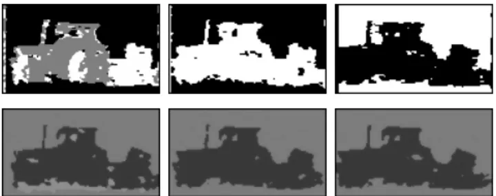
From top to bottom: (1) Input se- quence (with groundtruth overlaid); (2) Segmentation results from regular 3D MRFs with appearance-based observation model (544 pixels

The main forms of mobilities involved are the circulation of people, practices and ideas, the circula- tion of building types, the circulation of different kinds of media, such