Accurate analysis of memory latencies for WCET estimation

HAL Id: inria-00336530

https://hal.inria.fr/inria-00336530

Submitted on 4 Nov 2008

HAL is a multi-disciplinary open access

archive for the deposit and dissemination of

sci-entific research documents, whether they are

pub-lished or not. The documents may come from

L’archive ouverte pluridisciplinaire HAL, est

destinée au dépôt et à la diffusion de documents

scientifiques de niveau recherche, publiés ou non,

émanant des établissements d’enseignement et de

Accurate analysis of memory latencies for WCET

estimation

Roman Bourgade, Clément Ballabriga, Hugues Cassé, Christine Rochange,

Pascal Sainrat

To cite this version:

Roman Bourgade, Clément Ballabriga, Hugues Cassé, Christine Rochange, Pascal Sainrat. Accurate

analysis of memory latencies for WCET estimation. 16th International Conference on Real-Time and

Network Systems (RTNS 2008), Isabelle Puaut, Oct 2008, Rennes, France. �inria-00336530�

Accurate analysis of memory latencies for WCET estimation

Roman Bourgade, Clément Ballabriga, Hugues Cassé, Christine Rochange, Pascal Sainrat

Institut de Recherche en Informatique de Toulouse

CNRS – University of Toulouse

HiPEAC European Network of Excellence

{first.last}@irit.fr

Abstract

These last years, many researchers have proposed solutions to estimate the Worst-Case Execution Time of a critical application when it is run on modern hardware. Several schemes commonly implemented to improve performance have been considered so far in the context of static WCET analysis: pipelines, instruction caches, dynamic branch predictors, execution cores supporting out-of-order execution, etc. Comparatively, components that are external to the processor have received lesser attention. In particular, the latency of memory accesses is generally considered as a fixed value. Now, modern DRAM devices support the open page policy that reduces the memory latency when successive memory accesses address the same memory row. This scheme, also known as row buffer, induces variable memory latencies, depending on whether the access hits or misses in the row buffer. In this paper, we propose an algorithm to take the open page policy into account when estimating WCETs for a processor with an instruction cache. Experimental results show that WCET estimates are refined thanks to the consideration of tighter memory latencies instead of pessimistic values.

1. Introduction

As part of the design of a critical system, the Worst-Case Execution Time (WCET) of all the tasks with hard real-time constraints must be evaluated. The often huge number of possible execution paths in a task (related to the large number of possible input values) makes it impossible to determine the longest execution time by measurements if the WCET must be absolutely guaranteed as safe. This is why techniques based on static code analysis that allow deriving safe WCET upper bounds have been proposed [6]. Three steps are required: (1) information about the control flow must be provided by the user (through code annotations

[11]) or extracted automatically from the code [2][5][8][10]; (2) the execution times of sequential parts of code (basic blocks) must be determined taking into account the parameters of the target hardware [7][13][17][19]; (3) an upper bound of the execution time of the longest path must be derived from the results of steps 1 and 2. This final step is commonly done using the Implicit Path Enumeration Technique [12] that expresses the WCET computation problem as an Integer Linear Program. The objective function is to maximize the task execution time computed as the sum of the basic block execution times weighted by their execution counts. Constraints on these execution counts are built from the flow analysis. This is illustrated in Figure 1.

Now, several factors might make the execution times of basic blocks variable. In a pipelined processor, the state of the pipeline at the start of the block execution can affect the instruction scheduling and latencies (the state of the pipeline depends on the prefix path). The presence of history-based devices, like cache memories, also induces variable instruction latencies. The estimation of a block execution time (step 2) must take these factors into account. The result of this step can be the maximum execution time value of the basic block, which might lead to overestimate the task WCET, or the set of possible execution time values. In the latter case, the block execution count must be split into several counts related to the different execution time values and, in step 3, specific constraints on these counts must be derived. To illustrate this, let us consider a basic block that contains a single instruction, in a task that is to be executed on a microcontroller that features an instruction cache. We assume that the execution latency of the instruction is fixed. Then the basic block might have two different execution times, depending on whether the instruction fetch hits (tbh) or misses

(tbm) in the instruction cache. In the objective function

even = 0; odd = 0;

for (i=0 ; i<N ; i++) { if (i%2 == 0)

even++; else

odd++;

source code

compiler binarycode CFG-builder

B C D E A ILP formulation max T=xA.cA+ xB.cB+ xC.cC+ xD.cD+ xE.cE xA= 1 xA= xAB xB= xAB+ xEB xB= xBC+ xBD xC= xBC xC= xCE xD= xBD xD= xDE xE= xCE+ xDE xE= 1 + xEB flow analysis xEB! 255 xBC! 0.5 xB low-level analysis cA= … cB= … cC= … cD= … cE= … 1100101 ILP solver Tmax= … (WCET) with: xA= … xB= … xC= … xD= … xE= … solution N= input data

Figure 1. Overview of the IPET method to estimate Worst-Case Execution Times xbh.tbh + xbm.tbm and some constraints are added:

xbh + xbm = xb

and, for example,

xbm ! M

if an analysis of the cache behavior shows that the worst-case number of cache misses when fetching the instruction of block b is M. Note that if the processor is simple enough (in particular, if it executes instructions in the program order, as considered in the experimental part of this paper), the effect of a cache miss can be simply taken into account by adding the miss penalty (tp) due to the access memory, i.e. tbm = tbh + tp.

The problem of estimating the worst-case number of cache misses has been addressed in many papers: we will review them in Section 2. However, as far as we know, all these studies consider a fixed cache miss penalty, i.e. a fixed memory access time. Now, modern DRAM devices support the open page policy that reduces the latencies of sequential accesses to a same DRAM row (also called page). This scheme is sometimes called row buffer.

In this paper, our objective is to propose a technique to include tightly analyzed memory latencies in WCET estimations. Our algorithm is based on abstract

interpretation [4] and is based on methods previously proposed to analyze instruction caches [1][9][15][3]. Our contribution lies in the fact that we combine both analyses (at cache and memory levels).

The paper is organized as follows. Section 2 gives some background information on the memory open page policy and on state-of-the-art techniques used for the analysis of the instruction cache worst-case behavior. In Section 3, we explain our algorithm to analyze jointly the instruction cache and the memory row buffer. Section 4 provides some experimental results that show the improvement of the tightness of WCET estimations due to considering tight memory latencies. In Section 5, we discuss about possible extensions of our method. Finally, concluding remarks are given in Section 6.

2. Background

2.1. Memory hierarchy

The memory hierarchy is composed of several levels of storage, where the components at level n+1 generally have a slower data rate but a larger capacity

than those at level n, and where the data at level n are the copies of a subset of the data stored at level n+1. Usually, the lowest (fastest) levels correspond to cache memories and the highest level is some permanent storage (e.g. a disk or flash memory). The reason why the use of a memory hierarchy improves the average performance is that memory references are generally localized both in time and space.

Cache memories (particularly instruction caches) have been widely studied in the context of WCET estimation and techniques to analyze their behavior will be overviewed in Section 2.2. Here, we focus on the memory (DRAM) level.

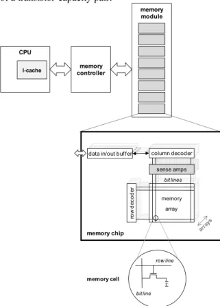
Figure 2 gives an overview of the main memory organization. On a cache miss, the main memory is accessed through the memory controller. It usually includes one or several memory modules, each of them being composed of several DRAM chips accessed in parallel to provide data of the desired width. Each of these chips is composed of one or several arrays of memory cells, accessed synchronously (then each chip provides several bits of data). A memory cell is made of a transistor-capacity pair. CPU memory controller memory module memory array ro w d ec o d er column decoder sense amps data in/out buffer

memory array ro w d ec o d er column decoder sense amps data in/out buffer

memory array ro w d ec o d er column decoder sense amps data in/out buffer

memory array ro w d ec o d er column decoder sense amps data in/out buffer

bit lines memory chip bit line row line memory cell I-cache

Figure 2. Main memory organization An access (read) to a memory array requires the following steps. First, all the bit lines must be

precharged to a logic level halfway between 0 and 1. Then the row containing the data (determined from the highest-order bits of the data address) is selected and all the bit values of this row (also called page) are recovered from the values stored on the capacitors through sense amplifiers. The lowest-order address bits are then used to select the bit (column) to be read.

The use of a row buffer consists in maintaining the last accessed row active. Whenever the next access is to the same row (row hit), only the selection of the new column is necessary. Otherwise (row miss), a new row must be read after a DRAM precharge. As a consequence, the latency of an access to the main memory depends on the content of the row buffer. On a row hit, the latency is reduced to tCAS (time interval

between the column access command and the start of data return). On a row miss, the latency is given by

tRP + tRCD + tCAS

where tRP is the time required to precharge a DRAM

array and tRCD is the time interval between the row

access command and the data ready at the sense amplifiers. Usual values for tCAS , tRCD and tRP are 2, 3

and 2 memory clocks respectively.

cmd read1 data1 read2 data2 read3 data3 read4 data4 cmd read1 data1 read2 data2 read3 data3 read4 data4 0 1 2 3 4 5 6 7 8 9 10 11 12 13 14 15

Figure 3. Latency of a memory access Figure 3 shows how the latency of a cache block fill from the main memory can be computed. In this example, we assume that a cache block is four times as wide as the memory bus. In the first case (upper chart), the access to the first part of the block is a row hit and then has a latency of tCAS. In the second case, it is a

miss and the latency of the first read is tRP + tRCD + tCAS. Note that only the access to the first

part of the block might miss in the row buffer (the other parts always hit) because of the following reasons: (a) each access concerns a single bit in the buffer (each bit of a word is in a different memory array and then in a different row buffer); (b) the number of bits in a row buffer required to fill a cache block is usually between 2 and 16; (c) common row widths are multiples of 16.

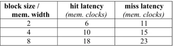
Considering the timing parameters numerical values given above, the possible latencies of a cache block fill are given in Table 1.

Table 1. Latencies of memory accesses block size / mem. width hit latency (mem. clocks) miss latency (mem. clocks) 2 6 11 4 10 15 8 18 23

2.2. Techniques for instruction cache analysis

In this section, we review the main state-of-the-art techniques proposed to analyze the behavior of the instruction cache for WCET estimation. These techniques are based on the classification of instruction fetches into categories (firstly defined in [15]): Always Hit (when each fetch is guaranteed to hit the cache), Always Miss and Not Classified (when the analysis is not able to predict a fixed behavior for this fetch). These categories are then used to build the ILP formulation as described in Section 1.

To improve the tightness of the analysis, the additional Persistent category (sometimes called First-Miss) can be considered. It concerns instructions that belong to a loop body and remain in the cache between successive iterations (but might miss at the first iteration). Several techniques have been proposed to identify Persistent instructions [9][15][3].

The categories are determined by performing an abstract interpretation [4] on a Control Flow Graph (CFG). Abstract Cache States (ACS) are computed in input and output of each basic block: an ACS is the set of concrete cache states that are possible at a given point during the execution of the program [1]. Two functions are used: the Update function computes the output ACS of a basic block from its input ACS, and the Join function merges the output ACS of all the predecessors of a basic block to produce its input ACS. The Update and Join functions are applied repeatedly until the algorithm reaches a fix point.

Three different analyses are done: the May, Must, and Persistence analyses. In each case, an ACS associates a set s of l-blocks1 _{(each one labeled with an}

age a) to each cache line. In the May (resp. Must) analysis, set s contains the l-blocks that may (resp. must) be in the cache, and the age a " [0 ,A[ of an l-block block is its youngest (resp. oldest) possible age. In the Persistence analysis, set s contains the l-blocks that may be in the cache, and the age a " [0 ,A[ U lT of

an l-block is its oldest possible age. The additional

1_{An l-block results from the projection of the CFG on the}

cache block map: a cache block that contains instructions belonging to n different basic blocks is considered as n l-blocks.

(oldest) virtual age lT stands for the l-blocks that may

have been fetched into the cache, and subsequently replaced. An l-block is persistent if it is in the Persistence ACS, and its age is not lT (i.e. once the

block has been fetched, it can never be replaced). Once built, the ACS are used to derive the instruction categories listed above.

3. Tight analysis of memory latencies

The row buffer behaves like a very simple cache that would have a single cache line. Then, at first sight, it should be analyzable using the same methods as for the instruction cache. Yet, the position of the row buffer in the memory hierarchy, behind the cache, requires taking the cache behavior into account.

3.1 Influence of the cache behavior

The memory row buffer behaves as a single-line direct-mapped cache. If an access to memory references the row that is active in the row buffer, its latency is shorter than when referencing another row. We use the following categories to analyze the worst-case behavior of the row buffer:

– Always Hit (RAH): the access is always fast because the row is active,

– Always Miss (RAM): the access is always slow because it never hits in the row buffer,

– Not Classified (RNC): if none of the previous categories applies (the behavior of the access is too complex to predict).

Since the row buffer is only accessed on cache misses, it should be analyzed with the same granularity as the cache, i.e. at the l-block level.

We introduce a new category: Row buffer Not Used (RNU) for the instructions fetches that hit in the cache. They do not have any effect on the row buffer state.

The category of an l-block is determined from its cache category and from the row buffer state before the l-block is fetched from memory.

The most trivial case is when the access is categorized AH in the cache: it is a cache hit and the row buffer is not accessed, which matches the definition of the RNU category.

An AM access always goes to the memory. If it can be proved that the referenced memory row is active in the buffer, the access category is RAH. On the contrary, if it can be proved that the row is not in the buffer, it is a RAM. Otherwise, we get an RNC.

The last cache-related category to consider is the less accurate one: NC (note that we do not handle loops in this analysis, so the cache FM category is considered as NC). It means that the access may result either in a

hit or in a miss (at different times). A trivial solution is to consider that the behavior of the row buffer cannot be predicted in this case and to select the RNC category.

To determine the state of a cache by static analysis, two analyses are performed:

– the Must analysis determines the cache state values at each program point, that are true whatever the execution path (the results of this analysis are used for classification to Always Hit), – the May analysis computes the different possible

values of the cache state at each program point considering all the possible execution paths (an access is categorized as Always Miss if the memory row is not in none of the possible states). In the simple case of the memory row buffer, only the May analysis is required, as shown in the following. Since the row buffer contains a single memory row, the May state consists in a set of possible rows. If it contains a single row, it means that all the paths access the same row and then the Must set equals the May set. On the contrary, if the May set contains several rows, it means that at least two execution paths load different rows and then, there is no way to prove that the row is active in the buffer before the access. For these reasons, we only need to perform the May analysis, as presented in the next section.

3.2 Analysis by abstract interpretation

Before starting the analysis, the list of memory rows involved in the execution of the program (MR) must be determined. This set is easily obtained by examining the program instructions addresses. Next, the concrete domain D where the real work is done can be defined. At any time, the row buffer contains a single memory row, then D = MR.

The abstract domain D’ gives the state of the row buffer at a program point for the abstract interpretation. As, the program usually contains many paths leading to that point, the state may contain a set of rows:

D’ = 2MR.

In the concrete domain, an Update function changes the state of the row buffer according to the memory accesses. It is very simple: if the row r " MR is read by the cache, the row buffer contents are replaced by r. In the abstract domain, it must be known (1) when a memory access is performed, according to the cache category and (2) which memory row is accessed (this is trivially deduced from the address).

Formally, the Update function U: D’ x MR#D’ defined as specified in the Table below (r is the memory row of the processed l-block):

cache category U(d, r)

AH d

AM {r}

FM, NC d U {r}

The two first rows are self explicit: cache category AH does not generate any memory access and the row buffer state is not changed; category AM results in a memory access and the referenced memory row becomes active in the row buffer. The last table row states that, since a memory access may or may not be generated for cache categories FM and NC, either the row buffer state is not changed, or the row is read. Thus the abstract domain of the May set contains the rows before the update and the referenced row.

Since the static analysis considers all the possible execution paths, path junction points (after a selection or at a loop entry, for example) can be identified. A Join function is required to merge the results of two joining paths: J: D’ x D’ # D’. In the May analysis, this function simply makes the union of the possible contents of the row buffer on both paths:

J(d1, d2) = d1 U d2

Finally, the abstract function $: D # D’ must be defined and used to prove the consistency of the analysis, i.e. that the Update and Join functions are monotonic on D’ so that the abstract result ever includes the concrete one. A complete partial order

)

,

,'

(

D

"

!

!

cache category

AH _If U(d, r)= d and U(d’, r)= d’

_d

_'

_#

_d

_d

_'

_#

_d

_d

_'

_#

_d

Once the May sets have been determined at each point of the program, they are used with the cache categories to derive the row buffer categories as explained in Section 3.1. The last step is to use these categories to improve the WCET ILP system.

3.3 ILP Formulation

Usually, the cost of cache misses for a given l-block is included in the WCET expression by adding the miss penalty (tp) weighted by the number of misses

(xicmiss). The IPET objective function is then:

WCET = max ( % xi .ti + % tp. xicmiss)

When considering a memory with a row buffer, the cache miss penalty has two different values, depending on whether the memory row is active in the buffer (tprhit) or not (tprmiss). The cache miss count is then split

into two variables (xicmiss = xirhit + xirmiss) and the

objective function becomes:

WCET = max ( % xi .ti

+ % t

. xi

+ % t

. xi

)

According to the row buffer category of the l-block, some constraints can be added:

– the RAH category indicates that no row buffer miss can occur, then xirmiss = 0.

– the RAM category states that the memory row reference always causes a miss, then xirhit = 0.

– the RNU category implies that xirhit = xirmiss = 0.

– the NC category does not impose any constraint on the ILP system.

As in the initial cache system, we can spare some variables by removing the xirhit. This is because the ILP

solver will minimize xirhit and maximize xirmiss that has

a greater weight (tprmiss). The objective function

becomes:

WCET = max ( % xi .ti

+ % t

. xi

+ % (t

- tp

) . xi

)

The trivial constraint becomes xirmiss ! xicmiss and the

constraint related to category RAM becomes xirmiss = xicmiss.

4. Experimental results

In this section, we provide some experimental results that show how an accurate modeling of the memory system is necessary to get tight WCET estimates.

4.1. Methodology

The algorithm presented in this paper has been

implemented within the OTAWA2 _framework

dedicated to static WCET analysis. The Worst-Case Execution Time of a task is estimated using the IPET algorithm [12].The worst-case execution costs of the basic blocks are derived from execution graphs [17] and the ILP formulation is augmented with constraints that bound the number of instruction cache misses and the number of memory row buffer misses. These numbers come from an analysis of the instruction cache similar to that described in [3] and from the analysis of the memory row buffer proposed in this paper, respectively.

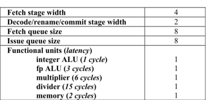
Hardware parameters. The experiments reported in this paper were carried out considering an in-order superscalar processor with the parameters given in Table 2. The processor includes a 2-way set-associative instruction cache with 16-byte cache lines and a capacity of 2 Kbytes. Note that the cache size has been set at deliberately small value to be significant with respect to the (small) size of the benchmarks (nevertheless the hit rate is the same as with a larger instruction cache for most of the benchmarks). It is assumed that no data cache is enabled and that the data are stored in an independent memory featuring a fixed access latency.

Table 2. Processor configuration

Fetch stage width 4

Decode/rename/commit stage width 2

Fetch queue size 8

Issue queue size 8

Functional units (latency) integer ALU (1 cycle) fp ALU (3 cycles) multiplier (6 cycles) divider (15 cycles) memory (2 cycles) 1 1 1 1 1

Table 3 lists the memory latencies considered for the experiments. We considered a memory clock cycle four times longer than the processor clock cycle, then the latencies are four times longer than those computed in Table 1. We considered four different memory row sizes: 128, 256, 512 and 1024 bytes.

2

Benchmarks. We used some benchmarks from the SNU suite3_{. They are listed in Table 4.}

Table 3. Memory access latencies

bus1 bus2 bus3

memory bus width (bits) 16 32 64

bus width / cache block size 2 4 8

hit 24 40 72

latencies

(processor clocks) miss 44 60 92

Table 4. Benchmarks

benchmark function # l-blocks

bs Binary search 25 crc CRC cyclic-redundancy check 167 fft1 Fast-Fourier transform using Cooly-Turkey algorithm 792

fibcall Fibonacci series 15

fir FIR filter with Gaussian

number generation 607

insertsort Insertion sort 37

jfdctint JPEG slow-but-accurate integer implementation of the forward DCT 115 lms LMS adaptative signal enhancement 457 ludcmp LU decomposition 315

matmul Matrix product 76

minver Matrix inversion 442

qurt Root computation of _{quadratic equations} 245

select N-th largest number

selection 160

4.2. Performance of the algorithm

Before examining how taking the presence of a row buffer into consideration can improve WCET estimates, let us have a look at the ratio of l-blocks concerned by our analysis. They are the l-blocks that are likely to access memory after a cache miss, i.e. the l-blocks that are not categorized as Always Hit by the cache analysis. Figure 4 shows the ratios observed for all the benchmarks used in our experiments. On average, 44% of the l-blocks must be categorized with respect to the row buffer.

3

http://archi.snu.ac.kr/realtime/benchmark/

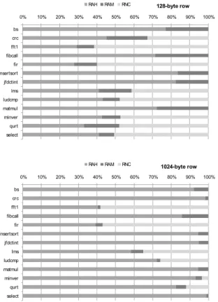
Figure 5 plots the different categories found for the different benchmarks, considering 128- and 1024-byte memory row sizes (note that the bus width has an impact on the memory latencies but not on the block categories). For all the applications, the ratio of l-blocks categorized as RowBuffer Not Classified (RNC) is significantly reduced when the memory row size is increased (on a mean, 14% of the l-blocks are RNC for a 128-byte memory row, and this number falls down to 8% for a 1024-byte memory row). The decrease is particularly significant for the minver, qurt and select codes. An explanation to this might be that the core of these codes fit in a 1024-byte

memory row and then the l-blocks become

categorizable. Note that, for all the benchmarks, the improvement of the categorization rate is in favor of the RowBuffer Always Hit (RAH) category. This is due to the fact that wide memory rows are better to capture spatial locality.

Figure 4. Ratio of l-blocks that might use the row buffer

The categories determined by our algorithm are used to include precise values for the memory latencies in WCET estimates (a short latency is considered for the l-blocks that are found to always hit in the row buffer). In Figure 6, the improvement of WCET estimates reached with our algorithm on is shown as a function of the size of the memory row and of the bus width. As expected, the gain is higher for a wide bus: this is because the number of memory accesses required for a cache block fill is smaller and then the overhead of a miss in the row buffer is lower compared to the global latency (20 cycles over 24 for a 64-bit bus, against 20 cycles over 72 for a 16-bit bus, as specified in Table 3. As a result, systematically considering long latencies (when the row buffer is not taken into account) is more pessimistic for wide busses.

0% 10% 20% 30% 40% 50% 60% 70% 80% 90% 100% bs crc fft1 fibcall fir insertsort jfdctint lms ludcmp matmul minver qurt select 128-byte row RAH RAM RNC 0% 10% 20% 30% 40% 50% 60% 70% 80% 90% 100% bs crc fft1 fibcall fir insertsort jfdctint lms ludcmp matmul minver qurt select 1024-byte row RAH RAM RNC

Figure 5. Categories found for 128- and 1024-byte memory row sizes

16 32 64 0% 2% 4% 6% 8% 10% 12% 14% 16% 128 256 512 1024 W C E T im p ro ve m en t

Figure 6. Average improvement of the WCET estimates

Figure 7 and Figure 8 show the impact of those two parameters (row size and bus width) on each of the benchmarks. The value of the second parameter (which is fixed here) has no impact on the shape of the curves. It can be observed that the improvement increases with the bus width for all the benchmarks. Most of the

benchmarks also draw a benefit from the analysis of the row buffer that is more significant when the memory row is wide. This is due to the fact that large row sizes allow a more precise categorization of the memory accesses. The improvement is spectacular for the minver, qurt and select application that have a sensibly better ratio of categorization for a 1024-byte row than for a 128-byte row.

0% 5% 10% 15% 20% 25% 30% 35% 40%

16 bits 32 bits 64 bits

Figure 7. WCET improvement as a function of the bus width (256-byte memory row)

0% 5% 10% 15% 20% 25% 30%

128 bytes 256 bytes 512 bytes 1024 bytes

Figure 8. WCET improvement as a function of the memory row size (32-bit bus)

5. Possible extensions of this work

Although it seems that the analysis of a memory row buffer has not been investigated yet, Mueller has proposed to apply its cache abstract simulation to L2 instruction caches [16]. He proposed two techniques to compute the categories for L2 cache accesses but no experimentation results are provided. As far as we know, L2 caches have still not been analyzed using techniques based on abstract interpretation. At first sight, the memory row buffer analyzed in this paper is not very different from a cache (it can be seen as a

cache with a single cache line). Then the analysis of an instruction cache coupled to a memory row buffer does not seem very different from a 2-level cache hierarchy (except that our second level is extremely simple here). In this section, we discuss whether our algorithm used to analyze the row buffer could be used or extended to analyze a two-level cache hierarchy. We highlight two main issues that might prevent from such a generalization.

First, there is a significant difference between the L1 cache and row buffer analyses: the latter is performed through the filter made of the categories determined by the former. The row buffer analysis is indeed impacted by the inaccuracies introduced by its own passes on one hand, and by the L1 cache analysis on the other hand. For example, each time an l-block is categorized as NC or FM for the L1 cache, two cases must be considered: the memory row may or not be active in the row buffer. The extreme simplicity of the row buffer (a single active row) reduces the range of the error as it is likely that the next memory access quickly results in a precise state that bounds the impact of the inaccuracy. If the algorithm proposed in this paper was to be extended to support L2 caches (instead of a memory row buffer), it would be necessary to evaluate the negative impact of both analyses to assert that the approach still gives useful results.

The second issue concerns the use of the Persistence analysis to get tight results in the cache analysis. The Persistence analysis allows benefiting from the code temporal locality and earlier work has shown that it can significantly improve the accuracy of WCET estimates [9][3]. We have not used the Persistence analysis in our row buffer analysis as accesses to the memory (on cache misses) are not likely to exhibit as much temporal locality as accesses to the cache. To extend our approach to support L2 caches, it would be necessary to implement the Persistence analysis. Determining whether the results obtained through the filter of the L1 categories remain useful is left for future work.

Another issue would be to take into account the accesses to data. In this paper, we have considered separate instruction and data memories so that the behavior of the row buffer for instruction accesses is not disturbed by data accesses. Taking into account the interferences due to data loads could be challenging. However, before tackling this problem, it is necessary to be able to analyze data caches, which is still an open issue at this time due to the difficulty of determining some of the data addresses during static analysis (however, some techniques provide some support for simple data indexing [14][18]).

6. Conclusion

To compute a safe and tight estimation of the Worst-Case Execution Time of a critical task, it is necessary to take into account every parameter of the target hardware. Various approaches have been proposed these last years to analyze the worst-case behavior of modern processors that include one or several pipelines, a branch predictor, cache memories, a dynamic instruction scheduler, etc. On the other hand, the memory system has not been much studied so far and the latency of memory accesses is generally considered as a fixed value. Now, modern DRAM devices support some mechanisms that improve the access rate by exploiting the temporal and spatial locality of the references. The row buffer, also referred to as open page policy, is one of these mechanisms. Whenever a piece of data is accessed, the entire memory row is maintained active until the next reference which can be served faster if it addresses the same row.

If the target processor does not have an instruction cache, the row buffer can be analyzed the same way as a very simple cache. But, when coupled to an instruction cache, the analysis of the row buffer requires a specific algorithm since not all of the instructions fetches go to memory (only those that miss in the instruction cache). In this paper, we have proposed such an algorithm based on an abstract interpretation of the application code.

Experimental results show that our algorithm is efficient in categorizing the behavior of the row buffer for a significant ratio of the accesses to memory. On average, 63% (84%) of the l-blocks are classified as RowBuffer Always Hit or RowBuffer Always Miss for a 128-byte (resp. 1024-byte) memory row width. The ratio of l-blocks that are determined as always hitting in the row buffer is very high (on average, 53% for a 128-byte row and 80% for a 1024-byte row). For each of the corresponding memory accesses, a short latency is accounted for in the estimated WCET. As a result, the estimated WCET is tighter as when the row buffer is ignored. Our results show that the mean improvement ranges from 6% (128-byte memory row and 16-bit bus) to 15% (1024-byte memory row and 64-bit bus). For some benchmarks, it reaches up to 34%.

As discussed in the paper, extending the proposed solution to support multi-level cache hierarchies would require further investigation, mainly to assert whether the accuracy of the results is acceptable. This will be part of our future work.

References

[1] M. Alt, C. Ferdinand, F. Martin, R. Wilhelm, “Cache Behavior Prediction by Abstract Interpretation”, Static Analysis Symposium, 1996.

[2] P. Altenbernd, “On the false path problem in hard real-time programs”, 8th _{Euromicro Workshop on Real-Time}

Systems, 1996.

[3] C. Ballabriga, H. Cassé, “Improving the First-Miss Computation in Set-Associative Instruction Caches”, Euromicro Conference on Real-Time Systems, 2008. [4] P. Cousot, R. Cousot, “Static Determination of Dynamic Properties of Programs”, 2nd _{Int’l Symposium on}

Programming, 1976.

[5] C. Cullmann, F. Martin, “Data-Flow Based Detection of Loop Bounds”, 7th _{Workshop on WCET Analysis, 2007.}

[6] J. Engblom, A. Ermedahl, M. Sjödin, J. Gustafsson, H. Hansson, “Towards Industry-Strength Worst Case Execution Time Analysis”, ASTEC 99/02 Report, 1999.

[7] J. Engblom, “Processor Pipelines and and Static Worst-Case Execution Time Analysis”, Ph.D. thesis, University of Uppsala, 2002

[8] A. Ermedahl, C. Sandberg, J. Gustafsson, S. Bygde, B. Lisper, “Loop Bound Analysis based on a Combination of Program Slicing, Abstract Interpretation, and Invariant Analysis”, 7th _{Workshop on WCET Analysis, 2007.}

[9] C. Ferdinand, F. Martin, R. Wilhelm, “Applying Compiler Techniques to Cache Behavior Prediction”, ACM SIGPLAN Workshop on Languages, Compilers and Tool Support for Real-Time Systems, 1997.

[10] N. Holsti, “Analysing Switch-Case Tables by Partial Evaluation”, 7th _{Workshop on WCET Analysis, 2007.}

[11] R. Kirner, J. Knoop, A. Prantl, M. Schordan, I. Wenzel, “WCET Analysis: The Annotation Language Challenge”,

7th _{Workshop on WCET Analysis, 2007.}

[12] Y.-T. S. Li, S. Malik, “Performance Analysis of Embedded Software using Implicit Path Enumeration”, Workshop on Languages, Compilers, and Tools for Real-time Systems, 1995.

[13] X. Li, A. Roychoudhury, T. Mitra, “Modeling out-of-order processors for WCET analysis”, Real-Time Systems, 34(3), 2006.

[14] T. Lundqvist, P. Stenström, “A method to improve the estimated worst-case performance of data caching”, Int’l Conference on Real-Time Computing Systems and Applications (RTCSA), 1999.

[15] F. Mueller, D. Whalley, “Fast Instruction Cache Analysis via Static Cache Simulation”, 28th _Annual

Simulation Symposium, 1995

[16] F. Mueller, “Timing Predictions for Multi-Level Caches”, ACM SIGPLAN Workshop on Language, Compiler, and Tool Support for Real-Time Systems, 1997.

[17] C. Rochange, P. Sainrat, “A Context-Parameterized Model for Static Analysis of Execution Times”, Transactions on HiPEAC, 2(3), Springer, 2007.

[18] J. Staschulat, R. Ernst, “Worst case timing analysis of input dependent data cache behavior”, Euromicro Conference on Real-Time Systems, 2006.

[19] S. Thesing, “Safe and Precise WCET Determination by Abstract Interpretation of Pipeline Models”, PhD thesis, Universität des Saarlandes, 2004.