HAL Id: hal-02874876
https://hal.archives-ouvertes.fr/hal-02874876
Submitted on 19 Jun 2020
HAL is a multi-disciplinary open access
archive for the deposit and dissemination of
sci-entific research documents, whether they are
pub-lished or not. The documents may come from
teaching and research institutions in France or
abroad, or from public or private research centers.
L’archive ouverte pluridisciplinaire HAL, est
destinée au dépôt et à la diffusion de documents
scientifiques de niveau recherche, publiés ou non,
émanant des établissements d’enseignement et de
recherche français ou étrangers, des laboratoires
publics ou privés.
The impact of coarse-grain protrusion on near-bed
hydrodynamics
David Raus, Frédéric Moulin, Olivier Eiff
To cite this version:
David Raus, Frédéric Moulin, Olivier Eiff. The impact of coarse-grain protrusion on near-bed
hy-drodynamics. Journal of Geophysical Research: Earth Surface, American Geophysical Union/Wiley,
2019, 124 (7), pp.1854-1877. �10.1029/2018JF004751�. �hal-02874876�
OATAO is an open access repository that collects the work of Toulouse
researchers and makes it freely available over the web where possible
Any correspondence concerning this service should be sent
to the repository administrator:
tech-oatao@listes-diff.inp-toulouse.fr
This is an author’s version published in:
http://oatao.univ-toulouse.fr/24269
To cite this version:
Reusch, David and Moulin, Frédéric Y. and Eiff, Olivier The
impact of coarse-grain protrusion on near-bed
hydrodynamics. (2019) Journal of Geophysical Research:
Earth Surface, 124 (7). 1854-1877. ISSN 1854–1877
Official URL:
https://doi.org/10.1029/ 2018JF004751
The Impact of Coarse-Grain Protrusion on Near-Bed
Hydrodynamics
David Raus1, Frédéric Yann Moulin1 , and Olivier Eiff2
1Institut de Mécanique des Fluides de Toulouse, Université de Toulouse, CNRS-Toulouse, Toulouse, France, 2Karlsruher Institut für Technologie, Karlsruhe, Germany
Abstract
In steep rivers, sediment is often transported over immobile cobbles and boulders. Previous studies of such conditions have observed that the entrainment rate of the mobile sediment strongly depends on the level of protrusion of the immobile grains. Here experiments are conducted in a laboratory flume in order to quantify how different levels of protrusion of large aggregates above a fixed fine-sediment bed, modeled as a patch of hemispheres, modify the local hydrodynamics near the fine-sediment bed. Five protrusion levels defined by P = k∕R = {0%, 20%, 40%, 60%, 80%} were investigated, where k is the protrusion height and R the radius. For small protrusion (P = 20%), enhanced shear stress and turbulence intensity on the fine-sediment bed is observed as the mixing layer generated at the hemisphere top impacts the fine-sediment bed. Moreover, sweep events generated near the top of the hemispheres reach the fine-sediment bed. For large protrusions (P ≥ 60%), the mixing layer generated near the top of the hemispheres does not reach the fine grains with the consequence that the shear stress drops. The remaining turbulence near the fine-sediment bed, although enhanced by the wakes generated by the hemispherical caps, is quasi-isotropic. The transition between these two distinct near-bed flow regimes is found to be around P = 40%, corresponding to the protrusion levels observed by Grams and Wilcock (2014, https://doi.org/10.1002/2013JF002925) above which the erosion of fine sediment ceases.1. Introduction
Wide grain-size distributions can cause predicted bed-load transport rates to be inaccurate (e.g., Yager et al., 2007). If the sediment bed consists of bimodal granular media with a large size ratio, segregation of the gran-ular media can lead larger aggregates to move toward the surface and protrude through the finer sediment. Thus, stream beds often consist of fine sediment being transported over coarse aggregates including large gravel, cobbles, or boulders, which are not set into motion by the flow except by extreme events. Clearly, the motion of the finer grains inside the interfacial sublayer of the immobile aggregates depends on the level of protrusion and spatial density of the aggregates. The interfacial sublayer is the flow region below the top of the aggregates or roughness elements, following the definition of Nikora et al. (2001). While the presence of large aggregates increases the total shear stress acting on the bed composed of aggregates and fine-sediment flow (i.e., the flow resistance), it is not fully available to set the finer sediment in motion (Einstein & Banks, 1950; Raupach et al., 1993; Smith & McLean, 1977; Yager et al., 2007). Most of the total shear stress is spent on the form drag of the larger aggregates, while only a small portion remains for the fine-sediment bed. Such drag partition was proposed early on in the context of eolian canopies without sediment by Marshall (1971) who measured the stress partitioning in a wind tunnel and Raupach (1992) who developed a partitioning model.
Numerous authors use spatial averaging of the turbulent and mean velocities in order to analyze the three-dimensional mean flow inside the roughness sublayer (e.g., Florens et al., 2013; Nikora et al., 2001) in a one-dimensional manner. Pokrajac et al. (2006), for instance, describe how the time- and space-averaged total shear stress varies with elevation above the bed, exhibiting a maximum value at elevations near the crest of the roughness element and decreasing below the crest as fluid momentum is increasingly trans-ferred to the roughness elements through form and viscous drag. The shear stress acting on the bed at the bottom of the interfacial sublayer (i.e., on the fine-sediment bed) is thus weaker than the total shear stress. This is particularly important for low submerged flows.
The effect of the presence of immobile roughness elements on sediment transport was first studied in aeolian conditions. Gillette and Stockton (1989) and Iversen et al. (1991) investigated the protection effect of
immo-Key Points:
• The local hydrodynamics over fixed small grains for varying protrusion of immobile coarse grains, modeled by hemispheres, is investigated via particle image velocimetry • A strong increase of the local shear
stress for small protrusion levels around 20% is observed, which Raupach's drag partition model cannot predict
• For protrusion levels higher than about 50%, a reduction of the turbulent normal and shear stresses as well as the latter's quadrant distribution is observed, all suggest-ing reduced grain mobility
bile coarse inclusions on transport by saltation. They showed that, for a fixed level of exposure of the coarse inclusions, the threshold friction velocity (that is required for particle motion) increases with the planar density of the coarse inclusions, indicating a protection or sheltering effect. Laboratory studies (Al-Awadhi & Willetts, 1999) and field studies (Gillies et al., 2006) have confirmed these observations. In rivers with a poorly sorted sediment bed, this increase of the threshold friction velocity is also observed (Schneider et al., 2015). Ferguson (2012) found that this increase of the threshold friction velocity has a clear dependence on the d84∕d50ratio, where d84and d50are the particle sizes for which 84% and 50% of the sediment is finer, respectively. For a poorly sorted river sediment bed, Wiberg and Smith (1991) argue that the critical shear stress of the larger grains can be lower than that of the finer material because coarse grains on a fine bed will have relatively lower intergranular friction angles and are more exposed to the mean flow. The authors conclude that, consequently, the fine sediment can be set in motion once the coarser grains move, expos-ing the fine sediment to the flow and increasexpos-ing the near-bed shear stress due to the absence of form drag associated with the coarse grains. However, the authors note that the finest grains are also affected by the turbulent velocity fluctuations in the wake of the coarse grains, which can set the fine grains in motion through turbulent sweeps of the bed.
Other authors have focused more specifically on the flow conditions before the coarse grains are set in motion. In a laboratory study, Yager et al. (2007) investigated bedload transport over immobile roughness elements in a steep channel by varying the surface density of an array of staggered immobile spheres. The authors observed that the entrainment rate of finer particles decreases by increasing the level of protru-sion of the large immobile spheres or by increasing their spatial density. Grams and Wilcock (2007, 2014) studied suspended sediment transport over a layer of immobile coarse hemispheres. It appeared that trans-port occurred in two main modes: (1) patches of fine sediment fully covering the immobile elements and (2) entrainment of fine sediment in the interstitial spaces between the hemispheres. The results showed a strong dependence of fine-sediment transport on the protrusion level of the hemispheres.
This dependence of sediment entrainment on the level of protrusion of immobile roughness elements is not fully understood. Nickling and McKenna Neuman (1995) studied aeolian transport of fine sediment by saltation over a layer of immobile spheres, the spheres being initially fully covered by the sediment. The authors observed that when the immobile spheres start protruding, the sediment entrainment increases, in agreement with increasing total shear stress, and then decreases below the no-protrusion rate as the spheres are progressively exposed. This suggests competing sheltering and drag partitioning effects. Sim-ilarly, Grams and Wilcock (2007) measured the near-bed entrainment rate of fine sediment for different levels of protrusion of a layer of large hemispheres. They observed that the entrainment rate first increases for small protrusions and then decreases as the protrusion increases further, concluding that the transition in transport rates occurs when the large hemispheres protrude enough to shelter the sediment. Erosion was observed to persist for protrusion levels up to 50%. The explanation given by the authors is that the near-bed turbulence generated in the wake of the immobile hemispheres creates a locally strong increase of the bed shear stress, leading to enhanced transport. The same explanation was invoked in more recent experimental studies of Wren et al. (2011) and Grams and Wilcock (2014).
There are also bed configurations where the near-bed turbulence intensity (i.e., the normal stresses) increases, which can enhance the mobility and transport of fine sediments even if the bed shear stress decreases. Sutton and McKenna Neuman (2008b), for instance, observed such a variation of the ratio of normal stress to bed shear stress for flow around an array of cylinders on a smooth bed without particles. The influence of the near-bed turbulence intensity on sediment transport was investigated by Sumer et al. (2003). They showed that sediment entrainment is strongly dependent on the turbulence intensity near the bed when the turbulence is generated by an external source (as, e.g., the wake of an obstacle). Empirical sediment transport laws depending on the near-bed turbulence level have been suggested by Sumer et al. (2003), successfully applied for scour around an isolated hemisphere (Dixen et al., 2013) but not applied yet for the case of sediment transport in an array of immobile roughness elements where turbulence can also be enhanced due to the wakes of the immobile elements.
However, even for turbulent flows over homogeneous beds, grains are not set in motion by the time-averaged bed shear stress u′w′ but by instantaneous events near the bed that can create locally strong velocity
fluctuation cross products (u′w′) which are washed out when averaged (Sechet & le Guennec, 1999). In par-ticular, a strong correlation between intense sweep events (u′w′ < 0 with u′ > 0 and w′ < 0) near the bed
and sediment transport is observed (Nelson et al., 1995). Thus, the transport of fine sediments in an array of large immobile roughness elements is very likely to be subject to modifications of the instantaneous events reaching the fine-sediment bed since the generation of coherent flow structures is influenced by the bed roughness. For instance, coarse gravel has been shown to be responsible for an increase of sweeps near the fine-sediment bed, which could trigger fine grain motions (Hardy et al., 2010; Nelson et al., 2001). Similar effects are also suggested by the study of Chang et al. (2011) who investigated sediment transport in the lee of an obstacle. These authors showed that using the time-averaged bed shear stress underestimates the entrainment rate for flow around an in-stream rectangular cylinder at low angles of attack by a factor 2 to 3 compared with that estimated from the instantaneous bed shear stress. Finally, Papanicolaou et al. (2001) show how the generation of coherent flow structures is influenced by the spatial density of the bed rough-ness elements, with the frequency of the generation of turbulent-burst structures increasing as the density of bed roughness elements increases. Such modifications of the near-bed velocity time series would clearly impact the transport properties of the flow for fine sediment.
The goal of this study is to understand how the level of protrusion of an array of immobile large aggregates modifies the hydrodynamics near the fine-sediment bed. To this end, the flow is modeled in an open-channel flume using a patch of hemispheres at different levels of protrusion above a fixed bed of fine sediment (glued grains). Using particle image velocimetry (PIV) measurements, mean flow and turbulence statistics are obtained above the hemispheres as well as inside the interfacial sublayer, resolved down to the fine-sediment scale. For different levels of protrusion of the patch of hemispheres, the local bed-shear stress over the fine sediment as well as the local near-bed turbulence statistics are compared with the no-protrusion case. The experimental setup and PIV measurements are presented in section 2. The main features of the three-dimensional mean flow and the roughness sublayer structure are presented and discussed in section 3. In section 4, the local mean and turbulent hydrodynamics near the fixed fine-sediment bed between the pro-truding hemispheres is investigated. The relevance of these purely hydrodynamical results to help explain the fine-sediment transport rates observed in experiments conducted by others is discussed in section 5. Conclusions and perspectives are drawn in section 6. In Appendix A, complementary results from a quad-rant analysis performed near the fine-sediment bed and near the hemispheres' top are presented, showing how the penetration of coherent structures inside the interfacial sublayer evolves with the protrusion level.
2. Experimental Setup
The experiments were conducted in an 11-m-long, 0.5-m-wide, 0.2-m-deep horizontal flume at the Institut de Mécanique des Fluides de Toulouse. The bed was covered by glued fine sediment from 2.3 m upstream of the measurement section up to 0.45 m downstream (Figure 1a). The glued fine sediment was made of plastic particles with d50 =2.2 mm and d90 =2.9 mm, where d90is the particle size for which 90% of the sediment is finer. In the measurement section, four patches of 3-D-printed spherical caps were screwed onto the immobile fine-sediment bed, and four scenarios were examined (details below). The caps had a radius
R =2cm and were fixed in a square arrangement of 7 × 5 caps plus a final row of five caps, as illustrated in Figure 1c, with a spacing l = 4.5 cm = 2.25R. The square arrangement was chosen so that PIV measurements (see below) down to the fine-sediment bed could be performed without the caps blocking the view of the instrument, at least in the alleys between the spherical caps.
The protrusion P of a spherical cap is defined as the ratio of the protruding height k above the fine-grained sediment bed to the full vertical radius R of the spherical cap:
P = k
R, (1)
where P = 100% corresponds to a completely uncovered hemisphere. In each patch, all the spherical caps have the same protrusion level for five different cases (P = 0%, P = 20%, P = 40%, P = 60%, and P = 80%). Measurements at P = 0% represent those for the glued fine-sediment bed without any caps.
The x, y, and z axes are defined, respectively, as the streamwise, transverse, and vertical directions. Here
z = 0is taken at the average position of the fine-sediment flow interface as measured by the PIV camera (see Figure 1b). The water depth D, measured between the fine-sediment bed position z = 0 and the water surface, is maintained constant for all experiments with a value of D = 0.125 m.
Figure 1. (a) Top view of the flume and positions of the patch of spherical caps (white circles) and glued sediment (gray shaded). (b) Zoomed side view of the patch. (c) Top view of an elemental pattern of spherical caps and positions of the laser sheets, A and C.
Instantaneous velocity fields were obtained by performing PIV measurements with a 16-bit high-resolution PCO Edge camera with a sensor size 2, 160 × 2, 560 pixels, in two wall-normal flow-parallel planes: plane
Cin the center of the patch of hemispheres, crossing two crests of the caps, and plane A in the adjoining downstream alley between the spherical caps (see Figure 1c). With the chosen camera angle, two hidden zones were present in plane A, since the spherical caps blocked the near bed region. The PIV fields were centered between the fourth row and the fifth row of spherical caps, where the flow is assumed to be fully developed inside the interfacial sublayer. The flow was seeded with 10-μm Dantec hollow glass spheres and illuminated with a laser-sheet generated by a 2×30 mJ Nd:Yag Quantel Twins Ultra laser and introduced via a set of mirrors from above. In order to reduce laser-sheet fluctuations, the sheet penetrated the free surface through a very slender glass window skimming the water surface, minimizing flow disturbances. To assure statistical convergence of the measurements, 5,000 statistically independent instantaneous velocity fields were recorded at the frequency f = 3 Hz for each case. The velocity fields were computed via an in-house software (CPIV-IMFT), with 16×16 pixels interrogation boxes with 50% overlap, the resolution of the images being 0.024 mm per pixel. The grid spacing was therefore 0.2 mm.
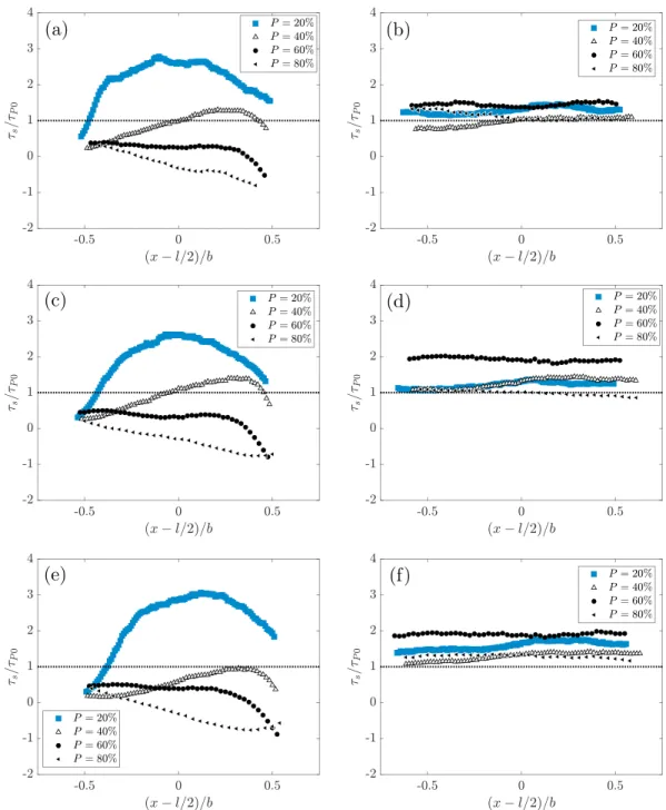
The bulk velocity is defined as Ub= Q∕(BD), where B = 50 cm is the width of the flume and Q the water discharge. Three discharges were investigated, Q = {6.6, 9.2, 13.7} L/s, for each of the five protrusion levels
P = {0, 20, 40, 60, 80}%; see Table 1. The flow discharge Q was chosen in order to obtain fully rough turbulent flow conditions. Two Reynolds numbers (also in Table 1) can be defined:
ReD=UbD∕𝜈, (2)
Rek=Ukk∕𝜈, (3)
where Ukis the double-averaged (i.e., temporal and spatial averaging in the horizontal directions) longitu-dinal velocity at the spherical caps' top (z = k) and𝜈 the kinematic viscosity of the fluid.
The chosen water depth D and the hemisphere's radius R are close to the values in Graba et al. (2010), where flow uniformity in the transverse direction in the same flume was verified. As in this earlier study, the effective channel-width to water-depth aspect ratio, B∕(D−k), is above 4. Combined with the fully rough beds, the flow near the center of the channel is therefore only weakly affected by the secondary currents generated by the lateral walls and is so essentially two-dimensional. The radius R of the hemispheres was chosen to keep the relative submergence D∕k for the highest protrusion (P = 80%) high enough to avoid low
Table 1 Experimental Parameters Experiment P(%) k(m) D∕k 𝜆f 𝜆p Q(L/s) Ub(cm/s) Fr ReD×103 Re k P0Q14 0 0 0 0 0 13.7 22.4 0.202 27.7 — P20Q14 20 0.004 31.3 0.032 0.22 13.7 22.4 0.204 27.7 489 P40Q14 40 0.008 15.6 0.088 0.40 13.7 22.4 0.206 27.7 1027 P60Q14 60 0.012 10.4 0.16 0.52 13.7 22.4 0.210 27.7 1449 P80Q14 80 0.016 7.8 0.23 0.60 13.7 22.4 0.213 27.7 2191 P0Q9 0 0 0 0 0 9.2 15.0 0.136 18.6 — P20Q9 20 0.004 31.3 0.032 0.22 9.2 15.0 0.137 18.6 345 P40Q9 40 0.008 15.6 0.088 0.40 9.2 15.0 0.138 18.6 685 P60Q9 60 0.012 10.4 0.16 0.52 9.2 15.0 0.141 18.6 1157 P80Q9 80 0.016 7.8 0.23 0.60 9.2 15.0 0.143 18.6 1427 P0Q7 0 0 0 0 0 6.6 10.8 0.097 13.3 — P20Q7 20 0.004 31.3 0.032 0.22 6.6 10.8 0.098 13.3 253 P40Q7 40 0.008 15.6 0.088 0.40 6.6 10.8 0.099 13.3 481 P60Q7 60 0.012 10.4 0.16 0.52 6.6 10.8 0.101 13.3 834 P80Q7 80 0.016 7.8 0.23 0.60 6.6 10.8 0.102 13.3 993
Note. P=k∕Ris the protrusion; k is the caps' protrusion height; D∕kis the relative submergence with D the water depth;𝜆f =nSf∕Sis the frontal density
and𝜆p=nSp∕Sis the planar density with n the number of roughness elements of frontal area Sfand plane area Spcovering the surface S; Q is the discharge;
Ub=Q∕(BD)is the bulk velocity;Fr = Ub∕√gDis the Froude number; ReD=UbD∕𝜈is the bulk Reynolds number; and Rek=Ukk∕𝜈is the crest Reynolds number.
submergence effects. In Rouzes et al. (2018), low submergence effects are observed in the log law parameters with an array of cubes for D∕k below 6.7, with values of the hydraulic roughness ksdiverging from values found in highly submerged flow conditions. With R = 2 cm chosen here, the lowest D∕k was equal to 7.8 so that all protrusions can be considered highly submerged. For the fine sediment, a scale separation with the hemispheres of at least one decade seemed reasonable to allow investigation of the spherical caps' interfacial layer without penetrating inside the fine sediment's roughness sublayer. Roughness sublayers are the highly inhomogeneous flow regions consisting of the interfacial sublayer and form-induced sublayer above the roughness elements, here the spherical caps or fine-sediment grains, and their thickness scales with the roughness element's vertical extent, that is, k or d50, respectively. With d50 = 2.2 mm and a PIV
spatial resolution of 0.2 mm, the spatial variations of the near-bed fine-sediment flow conditions inside the spherical caps' interfacial sublayer are investigated with a minimum of 20 measurement levels between the near-bed sediment and spherical caps' top for the lowest protrusion of P = 20% (k = 4mm). More quantitative analysis of the roughness sublayer thicknesses will be performed and discussed in the following sections.
3. Flow Structure
3.1. Time-Averaged Flow Fields
Figures 2a–2e and 2f–2j show the time-averaged longitudinal and vertical velocity fields, respectively, with superposed streamlines in the interfacial sublayer, for all levels of protrusion P = {0, 20, 40, 60, 80}%. For
P =20%, a recirculation is created in the wake of the spherical cap. This recirculation bubble is shorter than the distance between two spherical caps so that the spherical caps remain fully exposed to the free stream flow. For P = {40, 60, 80}%, the reattachment point of the recirculation, defined here as the position of zero streamwise and vertical velocity, is on the downstream spherical cap's surface. The reattachment posi-tion relative to the crest for P ≥ 40% is not dependent on the protrusion, implying that the portion of the spherical caps exposed to the outer flow is independent of the protrusion. It also appears that the magni-tude of the mean vertical velocity between the spherical caps depends on the distance at the base between them, the mean vertical velocity being minimum for P = 20% where the recirculation bubble is not limited by the next spherical cap. Depending on the level of interaction of the roughness elements with the flow, Morris (1955) delimits three regimes: isolated; wake interference, and skimming flow. In the case of urban canopies (i.e., rough beds of building-like cubes or cuboids), Grimmond and Oke (1999) show that for pla-nar densities of roughness elements𝜆p< 0.15 (where 𝜆p=nSp∕Swith n the number of roughness elements
Figure 2. Dimensionless mean velocity fields for ReD=27, 700(experiments PXXQ14) in plane C for all five protrusion levels P=0–80%, with (a–e) streamwise
velocity and (f–j) vertical velocity. The red dots show the position of the separation and reattachment points, and the green dots show the position of the center of the vortex. The overbar denotes time averaging.
of planar area Spcovering the surface S), the interaction between each roughness element and the flow is strong, as the roughness elements are fully exposed to the flow and act as wake generators, corresponding to the isolated regime. For 0.15 < 𝜆p < 0.35, referred to as the wake-interference flow regime, the shel-tering effect between the roughness elements becomes strong, and the momentum exchange between the roughness elements and the flow weakens. Finally, for𝜆p> 0.35, referred to as the skimming flow regime, a stable vortex forms and the interaction between the roughness elements and the outer flow diminishes fur-ther. A study of these three regimes for the specific case of spherical roughness elements was performed by Papanicolaou et al. (2001).
The planar densities for the nonzero protrusions P = {20, 40, 60, 80}% are 𝜆p = {0.22, 0.40, 0.52, 0.60}, respectively (see Table 1). For P = 20%, the flow topology suggests that the flow regime is still wake domi-nated (the isolated regime) since the wake generated by a spherical cap impacts the fine-sediment bed before reaching the next cap. Yet, since𝜆p=0.22, the criterion 𝜆p> 0.15 is satisfied for which the wake interfer-ence regime is expected, at least for urban canopies made of cuboid roughness elements. However, spherical caps for P = 20% are rounded objects with a wake topology clearly different from cuboids even at the same value of𝜆p. Therefore, for the bed of spherical caps, it is not impossible that the first transition proposed by Grimmond and Oke (1999) occurs for a protrusion between P = 20% and P = 40%, that is, for𝜆pbetween 0.22 and 0.40.
Figure 3 shows the local shear stress𝜏xz||local=𝜇(𝜕 ̄u∕𝜕z) − 𝜌𝑓u′w′in planes C and A normalized by𝜌𝑓u2⋆, wherēu is the time averaged streamwise velocity, u′and w′are the turbulent velocity fluctuations, u⋆is the friction velocity and𝜇 and 𝜌f are the viscosity and density of the fluid, respectively. We use here the term local to emphasize the fact that the shear stress is not spatially averaged. The friction velocity u⋆scales the turbulence acting at the top of the caps, with the scaling of the turbulence further discussed in section 3.3. For the no-protrusion case P = 0%, the inhomogeneities in the Reynolds shear stress reflect still-limited time convergence of the measurements (see next subsection). When the caps are present, the main contri-bution to the total shear stress in plane C is the turbulent mixing layer generated downstream from the top of the cap. For P = 20%, this turbulent mixing layer impacts the fine-sediment bed. It corresponds to the reattachment point located on the fine-sediment bed identified in the mean velocity fields. For larger pro-trusions, P ≥ 40%, the vertical turbulent mixing layer does not reach the fine-sediment bed anymore and impacts on the next spherical cap. The upper part of the mixing layer develops similarly for all the protru-sion levels investigated, supporting the hypothesis that the form-induced sublayer is not strongly modified
Figure 3. Dimensionless local shear stress𝜏xz||local∕𝜌𝑓u2⋆for ReD=27, 700for the different protrusion levels. (a–e) Measurements in plane C. (g–j)
Measurements in plane A. Gray areas are regions hidden from particle image velocimetry measurements.
with protrusion. However, the lower part of the mixing layer develops fully only for P ≥ 40%. For P = 20%, the impact on the fine-sediment bed limits its growth. It can also be observed in Figure 3 that the magnitude of the normalized shear stress𝜏xz||local∕𝜌𝑓u2⋆in the wake of the spherical caps decreases for P> 40%. Yet it should be noted that this decrease of the normalized shear stress can be explained by a stronger increase of the friction velocity𝜌𝑓u2
⋆relative to a weaker increase of the shear stress𝜏xz||local.
3.2. Double-Averaged Velocities and Spatially Averaged Turbulent Stresses
In the framework of the double-averaging methodology (e.g., Nikora et al., 2001), all time-averaged quanti-ties ̄𝜓(x, 𝑦, z) are decomposed into a time-averaged and spatially averaged component ⟨ ̄𝜓⟩ and a dispersive component ̃𝜓, that is, ̄𝜓 = ⟨ ̄𝜓⟩ + ̃𝜓, where the brackets ⟨.⟩ denote spatial averaging in the horizontal direction and the∼ denotes spacial fluctuation. Here the spatial averaging is performed over an
elemen-tary periodic pattern (see Figure 1a) since the roughness elements' distribution is periodic. In particular, the double-averaged quantities are estimated by averaging at a given level z the measurements in planes A and
Cbetween two caps' crests when caps are present or by averaging along the longitudinal direction in plane
Cfor the no-protrusion case.
The resulting vertical profiles of the double-averaged longitudinal velocity⟨̄u⟩ are plotted in Figures 4a–4e for the five different protrusion levels and the three different Reynolds numbers. Above the caps (z> k), the longitudinal double-averaged velocity is well described by the logarithmic law:
⟨̄u⟩ = u⋆ 𝜅 ln ( z − d ks ) +Br, (4)
where u⋆is the friction velocity at z = k (discussed in section 3.3), d is the displacement height, ksis the equivalent-sand-roughness scale,𝜅 = 0.41 is the Von Kármán constant, and Br=8.48 for fully rough flows. The value of Brwas established by Nikuradse (1933) in order to obtain the correlation ks=d50with natural sediment beds. The presence of a low velocity flow in the interfacial sublayer (below z< k) is obvious in the vertical profiles plotted in Figures 4a–4e. An inflection point can be identified for P ≥ 40% near z = k, where the slope of the profiles reaches a local maximum. As for poorly sorted natural beds, the velocity profile deviates from the logarithmic form below the crests (Lamb et al., 2017; Wiberg & Smith, 1991). Wiberg and Smith (1991) conclude that the logarithmic profile starts somewhere between z = d50and d84when the full
Figure 4. Vertical profiles of double-averaged longitudinal velocity⟨̄u⟩for ReD=27, 700(black square), ReD=18, 600(empty circles) and ReD=13, 300(black triangle) and for (a) P=0%, (b) P=20%, (c) P=40%, (d) P=60%, and (e) P=80%. The horizontal dashed lines show the height of the spherical caps and the mean altitude of the glued fine sediment.
In the double-averaged longitudinal momentum equation, the total shear stress𝜏xz(z)includes the dispersive (or form-induced) stress −𝜌𝑓⟨̃u ̃w⟩. Thus, in the double-averaged framework, 𝜏xz(z)is given by
𝜏xz(z) = −𝜌𝑓⟨u′w′⟩ − 𝜌𝑓⟨̃u ̃w⟩ + 𝜇
𝜕⟨̄u⟩
𝜕z , (5)
that is, the sum of the spatially averaged Reynolds shear stress, the dispersive shear stress, and the double-averaged viscous shear stress. More detail on the estimation of the dispersive stress is given in Florens et al. (2013) and Rouzes et al. (2018).
The vertical profiles of the total shear stress𝜏xz for ReD = 27, 700 are plotted in Figures 5a–5e for the five different protrusion levels, respectively. For P = 0% (Figure 5a), the profile is linear as expected for a gravity-driven two-dimensional boundary layer. Also, for P = 0%,𝜏xzapproaches 0 at z∕D = 0.4, indicating
Figure 5. Vertical profiles of total shear stress𝜏xz(z)(•), Reynolds shear stress−𝜌𝑓⟨u′w′⟩(□), viscous shear stress𝜇⟨𝜕 ̄u∕𝜕z⟩(△), and dispersive shear stress −𝜌𝑓⟨̃u ̃w⟩(◦), for ReD=27, 700and (a) P=0%, (b) P=20%, (c) P=40%, (d) P=60%, and (e) P=80%. Linear fits of the lower and upper parts of the total shear stress, used to determine the height of the internal boundary layer, are plotted as gray straight lines. The horizontal dashed lines show the altitude of the spherical cap and the mean altitude of the glued fine sediment.
Table 2
Boundary Layer Parameters for All Regimes
Experiment P(%) 𝓁z(m) 𝛿IBL∕𝓁z 𝛿extrap∕𝓁z d∕𝓁z ks∕𝓁z hRS∕𝓁z zm∕𝓁z zM∕𝓁z zm𝜖∕𝓁z z𝜖M∕𝓁z (𝛿10%+d)∕𝓁z
P0Q14 0 0.0022 25.1 25.1 −0.24 1.14 0.50 1.11 2.07 0.67 3.38 6.2 P20Q14 20 0.0040 4.5 8.8 0.30 1.44 2.08 1.60 1.84 1.36 2.36 2.0 P40Q14 40 0.0080 2.8 4.2 0.64 1.02 2.75 1.36 1.46 1.22 1.75 1.6 P60Q14 60 0.0120 2.4 3.2 0.71 0.87 1.33 1.20 1.28 1.12 1.43 1.4 P80Q14 80 0.0160 1.9 2.4 0.74 0.86 1.69 1.12 1.17 1.08 1.28 1.4 P0Q9 0 0.0022 19.9 19.9 −0.05 1.30 0.64 3.25 3.60 2.56 4.65 6.9 P20Q9 20 0.0040 4.5 7.5 0.36 1.27 2.43 1.67 2.01 1.43 2.49 1.9 P40Q9 40 0.0080 2.8 3.9 0.65 1.06 2.38 1.39 1.53 1.22 1.82 1.7 P60Q9 60 0.0120 2.4 2.9 0.71 0.73 1.33 1.21 1.31 1.15 1.45 1.5 P80Q9 80 0.0160 1.9 2.3 0.78 0.74 1.63 1.15 1.22 1.10 1.33 1.4 P0Q7 0 0.0022 21.8 21.8 0.04 0.83 0.55 3.51 4.04 2.47 5.87 5.5 P20Q7 20 0.0040 4.5 7.2 0.38 1.27 3.75 1.72 1.96 1.43 2.58 2.1 P40Q7 40 0.0080 2.9 3.8 0.67 1.03 3.00 1.47 1.59 1.28 1.93 1.7 P60Q7 60 0.0120 2.3 2.8 0.74 0.56 1.42 1.23 1.32 1.15 1.47 1.4 P80Q7 80 0.0160 1.9 2.3 0.77 0.71 1.25 1.17 1.23 1.11 1.33 1.4
Note. 𝓁zis the vertical lengthscale of the rough bed, defined as equal to d50for the no-protrusion case (P=0%) and equal to k, the protruded height, for all other protrusion levels (P > 0%). The fitted logarithmic parameters are d, ksas well as the lower and upper bounds zmand zMobtained by minimizing the slope error with initially five points, following the approach of Rouzes et al. (2018).z𝜖mandz𝜖mare the lower and upper bounds of the logarithmic law using a spatial convergence error estimate𝜖⟨̄u⟩with 95% confidence. hRSis the roughness sublayer height computed from the spatial standard deviation of the mean and turbulence statistics as in Florens et al. (2013) and Rouzes et al. (2018).
the top of boundary layer, which implies that the boundary layer developing on the fine sediment is not fully developed.
When the spherical caps protrude (Figures 5b–5e), the total shear stress profiles𝜏xz(z)break into two linear slopes, the lower ones with a higher slope than the upper ones. In all cases,𝜏xz(z)reaches a maximum value near the top of the spherical caps. The lower portions of the profiles with the stronger slopes reveal the development of a new boundary layer generated by the caps growing inside the upstream boundary layer generated by the fine-sediment bed. For z< k below the caps' top, 𝜏xz(z)decreases, gradually reduced by the form and viscous drag induced by the caps and in accordance with the form and viscous drag terms in the double-averaged momentum equations inside the interfacial sublayer (e.g., Pokrajac et al., 2006).
The heights of the boundary layers developing on the patches were quantitatively determined using two approaches. The first height, noted𝛿extrap, was obtained by extrapolating a linear fit of the lower portion of
𝜏xz(z)up to𝜏xz=0. The second, noted𝛿IBL, was defined by the level of the change of slope of𝜏xz(z)and was obtained by the intersection of the linear fits of the lower and upper portions of𝜏xz(z). In Figures 5b–5e, these linear fits have also been plotted.
The resulting boundary layer heights are given in Table 2, normalized by the height k of the spherical caps for P> 0% or by the small grain median diameter d50for the no-protrusion case P = 0%. For completeness, the prediction for the equilibrium layer thickness proposed by Cheng and Castro (2002) who studied the development of an internal boundary layer in an atmospheric-type boundary layer was also computed, noted
𝛿10%(using equation P10 on Figure 10 of Cheng & Castro, 2002) by adding the displacement height d before normalizing with k, d being the altitude of the origin of the logarithmic section of the double-averaged longitudinal velocity. As seen in Table 2,𝛿10%gives the shortest estimations of the internal boundary layer height, followed by𝛿IBLand𝛿extrap. The heights will be discussed in section 3.4.
3.3. Logarithmic Law and Roughness Sublayer
The friction velocity u⋆scaling the turbulence above the interfacial sublayer (z> k) is determined by extrap-olating the total shear-stress profile to the top of the spherical caps (z = k) (Pokrajac et al., 2006; Rouzes et al., 2018). The roughness height ksand the displacement height d are then determined by fitting a logarithmic law on the vertical profiles of the double-averaged longitudinal velocity of Figure 4, considering only the
Figure 6. (a–d) Total spatial dispersion2Dt(black dots) and time convergence error𝜖̄𝜓(orange line), estimated here with a95% confidence interval, for the protrusion level P=0%. The dotted horizontal lines show the altitude of the highest grain's top. (e–h) Spatial dispersion2Dsfor the protrusion level P=0%. The red line represents z=d50, the altitude above the fine sediment chosen in the present study to estimate the bed flow conditions (see text). The dashed horizontal line shows the altitude of the highest grain's top.
region above the spherical caps (z > k) and following the constant 𝜅 method of Rouzes et al. (2018) with
𝜅 = 0.41. The values of the log law parameters u⋆, d, and ksfor the investigated regimes are given in Table 2, along with the lower and upper limits of the logarithmic law fit as defined and discussed in Rouzes et al. (2018).
The roughness sublayer for a turbulent flow over a rough bed is defined as the layer where the roughness elements induce mean-flow spatial heterogeneities. Following Florens et al. (2013) and Rouzes et al. (2018), the top of the roughness sublayer, noted hRS, is defined as the height where the nondimensional spatial standard-deviation 2Ds(̄𝜓(z))∕⟨ ̄𝜓(z)⟩ is equal to 5%. In order to remove the contribution of the time conver-gence error, Florens et al. (2013) showed that a good estimate of the spatial dispersion of a time-averaged quantity is given by
2Ds(̄𝜓(z)) = 2Dt(̄𝜓(z)) − 𝜖̄𝜓, (6) where Dt(̄𝜓(z)) =
√
⟨ ̃𝜓2(z)⟩ is the total spatial dispersion based on the double-average decomposition, and 𝜖̄𝜓is the time convergence error of the turbulent quantities due to the finite number of independent samples used in the time averaging. The time convergence errors are estimated using the confidence intervals of the mean and variance of the velocity signals and the estimated number of independent samples. In the present study, hRSis determined by the spatial standard deviation of the longitudinal mean velocity component, 2Ds(̄u(z))∕⟨ ̄𝜓(z)⟩. The normalized values for the different protrusion levels are given in Table 2.
The roughness sublayer for the no-protrusion case P = 0% deserves closer attention. The reason is that for the flows with emerging caps, two roughness sublayers coexist: one at the caps' scale and the other at the fine-sediment grain scale. In the next subsection, the spatial variations of the mean flow and turbulence quantities inside the cap's roughness sublayer will be investigated and must be distinguished from the spatial variations due to the fine grain roughness sublayer. Therefore, for P = 0%, the total spatial dispersions 2Dt and the time convergence errors𝜖̄𝜓are presented in Figures 6a–6d, for the relevant quantities, that is, the longitudinal velocity ̄u, the Reynolds shear stress −u′w′, and the streamwise and vertical normal stresses u′2and w′2. As in Florens et al. (2013), the total spatial dispersion 2D
ttends toward the time convergence error𝜖̄𝜓at some level above the bed. The effective spatial dispersion 2Dsplotted in Figures 6e–6h shows that
Figure 7. (a)k+
s of the patch plotted against the protrusion P. Dashed lines delimit the hydraulically smooth,
transitional and rough bed. (b) Equivalent sand roughness ksnormalized by the distance between hemispheres plotted against the protrusion P. The inset shows the evolution of ksnormalized by the height of the spherical caps k.
2Ds, unlike 2Dt, tends toward 0 at some level above the bed, in agreement with the concept of a roughness sublayer.
For the fine-sediment bed, the top of the roughness sublayer hRSbased upon the dispersion of the longitu-dinal mean velocity is roughly equal to d50∕2(see Table 2). However, as seen in Figures 6e–6h, dispersion remains higher for other quantities, in particular for −u′w′(Figure 6f). By choosing a reference altitude at z = d50(red line in Figures 6e–6h), the spatial dispersion 2Dsat that level is below 5% for ̄u, u′2, and w′2,
and below 10% for −u′w′. Therefore, an altitude of z = d
50above the fine-sediment bed appears to be a
good compromise between the requirements of being out of the fine-sediment bed roughness sublayer and still remaining close enough to the fine-sediment bed to quantify the local forcing on the fine grains. This altitude will be used to calculate the flow quantities near the bed in the presence of protrusions.
3.4. Effect of Patch Protrusion on the Vertical Structure of the Turbulent Boundary Layer
In Table 2, it can be seen that the relative submergence of the roughness elements𝛿extrap∕lzof the devel-oping boundary layer over the glued sediment bed for the no-protrusion case P = 0% is very high with
𝛿extrap∕lz = 𝛿extrap∕d50 in the range [19.9, 25.1] for the three Reynolds numbers investigated. As the caps protrude above the fine-sediment bed, the submergence of the caps relative to the cap-generated internal boundary layer decreases and drops to values as low as 1.9 for P = 80% using𝛿IBLas the boundary layer thick-ness. For a similar array of cubes with roughly the same frontal density, Rouzes et al. (2018) showed that the logarithmic law is still found for relative submergence ratios down to 1.5, the mimimum ratio investigated, and that it extends deep into the roughness sublayer. Here logarithmic laws are also found, including for the lowest submergence, and located very close to the cap's top while penetrating the roughness sublayer (see Table 2). Moreover, for low submergence flows with P ≥ 40%, the top of the logarithmic law is in very good accordance with the thickness of the equilibrium layer predicted by Cheng and Castro (2002) and slightly smaller for the more submerged flow at P = 20%.
The evolution of k+
s = ksu⋆∕𝜈 with P is plotted in Figure 7a. k+s = ksu⋆∕𝜈 compares the equivalent-sand-roughness scale to the thickness of the viscous sublayer of the equivalent hydraulically smooth flow. For P = 0% and the three Reynolds numbers investigated, 5< k+
s < 70, showing that the bed is in the transitionally rough regime for the no-protrusion case. For P = 20%, the bed becomes fully rough (i.e.,
k+
s > 70) for ReD=27, 700 but stays in the transitional regime for smaller Reynolds numbers. For greater protrusion levels of the patch, the bed becomes fully rough for all the Reynolds numbers investigated. The evolution of ks∕lwith P is plotted in Figure 7b, where l is the distance between the hemisphere. For fully rough turbulent boundary layers, ksis expected to be independent of the Reynolds number if the flow topology inside the roughness sublayer also remains the same. This is verified for P = 20% and P = 40% but not for P = 60% and P = 80%. In Rouzes et al. (2018), a dependence of kswith the relative submer-gence D∕k is observed, but all estimations of the relative submersubmer-gence in Table 2 (i.e.,𝛿IBL∕kand𝛿extrap∕k) are almost Reynolds-number independent for a fixed value of P and cannot be responsible for the differ-ent values of ks. Only a slight change of the flow topology in the roughness sublayer could explain this
Figure 8. (a) Evolution of the ratio𝜏b∕𝜏P0with the protrusion P. (b) Evolution of the ratio𝜏b∕𝜌𝑓u2⋆with the
protrusion P. The inset shows the evolution of the integrated porosity∫0k𝜙(z)dz∕kwith the protrusion P.
Reynolds number dependence. The flows around rounded objects like the present spherical caps are more subject to such dependence than roughness elements with sharp edges like cubes. However, the Reynolds number dependence does not mask the very clear trend in Figure 7b, where ks∕lincreases linearly with the protrusion P.
As discussed in Rouzes et al. (2018), one of the difficulties with low relative-submergence flows over rough beds is that the friction velocity used to fit the logarithmic law, estimated at the top of the spherical caps, is different from the one yielding the bed shear stress𝜏bwhich measures the total flow resistance in vertically integrated models. This bed shear stress associated with the total resistance of the bed (i.e., both the spherical caps and the fine-sediment bed) is given by (Pokrajac et al., 2006)
𝜏b=𝜌𝑓u2⋆ ( 1 + ( ∫k 0 𝜙(z)dz k ) k 𝛿extrap ) , (7)
where𝜙(z) is the porosity of the bed, equal to 1 above the interfacial sublayer, and lower than 1 inside the interfacial sublayer. Profiles of𝜙(z) required to calculate 𝜏bdepend of the protrusion P. At each level
z, the intersection of the horizontal plane with a protruding hemisphere is considered. The surface of the intersected hemisphere is calculated analytically and substracted from the periodic pattern area l2, yield-ing the fluid surface area at altitude z. The porosity at altitude z is then obtained by dividyield-ing this surface area by l2.
The evolution of𝜏b∕𝜏P0with protrusion P, where𝜏P0is a reference value of𝜏bcorresponding to P = 0%, is plotted in Figure 8a, and the evolution of𝜏b∕𝜌𝑓u2
⋆is plotted in Figure 8b. The integral term in front of k∕𝛿extrap in equation (7) has been plotted as a function of the protrusion in the inset of Figure 8b. It corresponds to the bed-averaged porosity, noted Φ, of the rough bottom. It decreases from unity for P = 0% to 0.59 for
P =100%, which is slightly larger than the value for a compact bed of spheres in a square arrangement (0.48). As the protrusion of the hemispheres increases, the drag acting on the caps becomes more important than the resistance of the fine-sediment bed and it can be seen accordingly in Figure 8a that𝜏b∕𝜏P0increases,
up to a ratio of 3 for P = 80%. The ratio𝜏b∕𝜌𝑓u2⋆in Figure 8b is also seen to increase with P, reaching 1.3 for P = 80%, but this is only due to the increasing low relative-submergence flow conditions, with𝛿IBL∕k ratios as low as 1.9 for P = 80%. As seen in equation (7), for increasingly submerged flows as k∕𝛿extrap→ 0,
𝜏b∕𝜌𝑓u2⋆approaches 1.
4. Near-Bed Hydrodynamics
4.1. Determining the Local Shear Stress on the Fine-Sediment Bed
In this section, the fine-sediment shear stress𝜏s, defined as the local shear stress acting on the bed of fine grains, is determined and compared to the total shear stress𝜏bcalculated from (7). The sediment shear stress
𝜏s is measured at the top of the rou ghness sublayer of the fine sediment (Nikora et al., 2001), that is, at
time-averaged quantities at the fine-grain scale. The local shear stress𝜏sacting on the fine-sediment bed is therefore estimated by 𝜏s≡ 𝜏xz||local(z = d50) =𝜇 𝜕 ̄ u 𝜕z||||z=d50 −𝜌𝑓(u′w′)| ||z=d50. (8)
Since the local shear stress is estimated at the top of the fine sediment's roughness sublayer, the dispersive stress is negligible. It should also be noted that estimating𝜏sat z = d50above the fine-sediment bed might
lead to small discrepancies for low relative submergence situations of the grains since the stress is not extrap-olated to the bottom of the grains. However, in the following, the local shear stress will be always compared to the value of the bed shear stress taken at z = d50without spherical caps, that is, to𝜏P0, to reveal the effect
of the presence of spherical caps.
4.2. Spatial Distribution of the Fine-Sediment Shear Stress
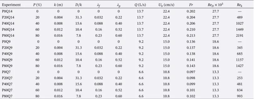
Longitudinal profiles of the fine-sediment shear stress𝜏snormalized by the total shear stress without spher-ical caps𝜏P0are plotted in Figures (9a, 9c, and 9e) for plane C and in Figures (9b, 9d, and 9f) for plane
Afor all protrusion levels P and Reynolds numbers. When𝜏s∕𝜏P0 < 1, the fine sediment is locally shel-tered from strong shear stress due the presence of the spherical caps. On the contrary, when𝜏s∕𝜏P0> 1, the fine-sediment bed is locally exposed to the enhanced shear stress generated by the presence of the caps. In plane A (see Figures 9b, 9d, and 9f), the shear-stress distribution on the fine-sediment bed is relatively uniform along the streamwise direction and is enhanced (𝜏s∕𝜏P0> 1) by the caps for all protrusions, with a
maximal enhancement for P = 60% at which𝜏s∕𝜏P0reaches 1.9 for ReD=27, 700 and 1.5 for ReD=13, 300. Similar enhanced shear stress has been observed between two side-by-side cylinders (Kim et al., 2014), in the leeside of a row of cylinders (Sutton & McKenna Neuman, 2008a) or in an array of cylinders (Sutton & McKenna Neuman, 2008b). Kim et al. (2014) show that when the distance between the two cylinders is smaller than 2.5 times the diameter of the cylinders, the two horseshoe vortices developing on each cylin-der can interact and create strong shear stress between the roughness elements. For an array of cylincylin-ders, Sutton and McKenna Neuman (2008b) explain that this effect persists if more rows of cylinders are present and that the effect of compression and acceleration of the flow between the roughness elements is addi-tive. Here in the interfacial sublayer, the same process occurs: Even if the double-averaged longitudinal velocity is reduced by the drag of protruding caps, this global reduction hides an increase of the mean lon-gitudinal velocity in plane A (which becomes a preferential path for the flow), enhancing the fine-sediment shear stress.
In plane C (see Figures 9a, 9c, and 9e), strong variations of𝜏s∕𝜏P0along the streamwise direction are observed for all protrusions, with zones of sheltering and zones of enhanced shear stress developing between the caps. The length of the protection zone is very small for P = 20% but increases with P and leads to fine sediment exposed to reduced shear stress along the entire bed in plane C for P = 60% and P = 80%. Similar sheltering zones were observed in the lee of an isolated hemisphere by Dixen et al. (2013). For P = 20%, a zone of strongly enhanced fine-sediment shear stress is observed midway along the distance between the spherical caps, with𝜏s∕𝜏P0reaching a maximum value of about 3 for the three Reynolds numbers investigated here.
This strong enhancement is clearly associated with the impact on the fine-sediment bed of the mixing layer generated at the top of the caps, as observed in Figure 3b and discussed in section 3.1. For P = 40%, a short distance of slightly enhanced shear stress appears close to the right spherical cap for ReD = 27, 700 and
ReD= 18, 600 (see Figures 9a and 9c). For ReD= 13, 300, this enhancement disappears, with a maximum value similar to that without caps (see Figure 9e). The evolution of the horizontal profiles of𝜏s∕𝜏P0in plane C
corresponds to the transition observed with P in Figures 2a–2e and 3a–3e, where the reattachment points of the recirculation cell (and thus the impact of the mixing layer) shift from being located on the fine-sediment bed between successive caps (P = 20%) to the front side of the downstream cap (P ≥ 60%). The P = 40% protrusion is an intermediate flow regime between these two situations, with a mixing-layer growth that still allows some enhancement of the fine-sediment shear stress: the reattachment point is already on the front side of the downstream cap but close enough to the fine bed sediment. The sediment is thus still influenced by the occurence of the mixing layer.
4.3. Spatial Distribution of the Near-Bed Turbulence Intensity
Sumer et al. (2003) showed how adding external near-bed turbulence to a flow can enhance grain entrain-ment. A way to take into account the level of turbulence for fine-sediment transport is to define the sediment
Figure 9. Horizontal profiles of fine-sediment shear stress𝜏sbetween the spherical caps, normalized with the
reference shear stress𝜏P0(measured in the no-protrusion case P=0%) for all protrusion P≥ 20%. ReD=27, 700in planes C (a) and A (b), ReD=18, 600in planes C (c) and A (d), and ReD=13, 300in planes C (e) and A (f). The longitudinal position is normalized by the spacing b at the base of protruding caps (Figure 1c).
shear stress directly via the turbulent kinetic energy near the fine-sediment bed TKEs. With this approach, a new estimate for the fine-sediment shear stress, noted𝜏s,TKEis given by
𝜏s,TKE=𝜌𝑓C TKEs=𝜌𝑓C2 (
u′2+v′2+w′2), (9)
where C is a constant. This constant is often chosen with a value equal to C = 0.19 (Nezu & Nakagawa, 1993; Soulsby, 1983) and corresponds to the amplitude of the exponential fits of the turbulent kinetic energy profiles in turbulent boundary layers when nondimensionalized by the friction velocity u⋆.
Figure 10. Horizontal profiles of fine-sediment shear stress𝜏s,TKEestimated with the turbulent kinetic energy between the spherical caps and normalized with the reference shear stress𝜏P0for all protrusion P≥ 20% for ReD=27, 700in (a) plane C and (b) plane A (Figure 1c).
Here the transverse velocity variance v′2is not available, so that the turbulent kinetic energy is estimated
following the suggestion of Nezu and Nakagawa (1993) with
TKE =1 2 1 0.72 ( u′2+w′2). (10)
It is then possible to determine the value of C from measurements without protrusion P = 0% at the level
z = d50chosen to investigate the near-bed fine-sediment flow conditions. Thus, C with TKEs =⟨TKE⟩(z =
d50)evaluated for P = 0% is given by
C|PO=
𝜏xz(z = d50) 𝜌𝑓⟨TKE⟩(z = d50)
. (11)
For the three different Reynolds numbers investigated, ReD= {13, 300, 18, 600, 27, 700}, the values of C|PO are found to be 0.24, 0.25, and 0.26, respectively. Therefore, to estimate𝜏s,TKEfor P ≥ 20% in equation (9), C =0.25 was chosen for all P, with TKEsevaluated at z = d50.
Horizontal profiles of the fine-sediment shear stress𝜏s,TKEcalculated with the near-bed turbulent kinetic energy are plotted in Figures 10a and 10b for planes C and A, respectively, and normalized by𝜏PO. The shape of these profiles for P = 20% and P = 40% are very similar to the shape of the profiles of𝜏s∕𝜏POin the corresponding Figures 9a and 9b. This indicates that for these flow regimes, both estimators reflect that the mixing layer impacts the fine-sediment bed (P = 20%) or the next cap's toe (for P = 40%), enhancing the near-bed fine-sediment shear stress in comparison with the no-protrusion case.
For P ≥ 60%, the two estimators give different yet complementary information in plane C. In Figure 9a, the fine-sediment shear stress𝜏s∕𝜏P0is low and becomes highly negative near the toe of the downstream cap, in accordance with the downward motion of the recirculation there, suggesting a sheltering effect, since grains will tend to move upstream in such a flow. In Figure 10a, the fine-sediment shear stess𝜏s,TKE∕𝜏PO remains high for P = 60%, with levels just below that of the no-protrusion case P = 0%. This indicates that for P ≥ 60%, the instantaneous velocity fluctuations are still high enough in the wake of the caps to trigger grain motion, but since𝜏sis then negative, this motion would then transport the grain upstream, toward more sheltered regions closer to the cap's lee face.
4.4. Double-Averaged and Maximum Near-Bed Fine-Sediment Shear Stress
Raupach et al. (1993) present a model for partitioning the bed shear stress𝜏bbetween immobile roughness elements and the surrounding erodible bed. Their approach examines both the spatial average and the local maximum of the shear stress on the fine-sediment bed relative to the total shear stress (their equations (11) and (15), respectively). The method requires determining drag coefficients for the fine sediment CSand the large roughness elements CR. For P = 0%, CScan be calculated from
Figure 11. (a) Variation of the double-averaged value of the shear stress over the fine-sediment bed at z=d50, normalized by the total bed shear stress. The blue line corresponds to the prediction based upon equation (11) of Raupach et al. (1993) for the shear stress averaged only on the fine-sediment surface (noted𝜏′
sin Raupach et al., 1993).
(b) Variation of the maximum value of the shear stress over the fine-sediment bed at z=d50, normalized by the total bed shear stress. The blue line corresponds to the computation of equation (15) of Raupach et al. (1993), with CR=0.3
and m=0.05, 0.1and 0.2.
which yields an average CS value of 0.0050 ± 0.0007 for the three Reynolds numbers examined in our experiments. Values of CRfor the drag force on an isolated spherical cap could not be inferred from our mea-surements. Instead, CR=0.3 for full hemispheres was used as suggested by Raupach et al. (1993) and it was assumed that the drag coefficient is not dependent on the protrusion level of the spherical caps.
Two comparisons with the predictive model of Raupach et al. (1993) are possible here: the variation of the double-averaged shear stress acting on the finer sediment,⟨𝜏s⟩, and the variation of the local maximum value of the shear stress acting on the finer sediment,𝜏s,max. Figure 11a shows the evolution of the ratio ⟨𝜏s⟩∕𝜏bas a function of P. As the spherical caps protrude through the finer sediment, it appears that the part of the total bed shear stress effectively acting on the finer sediment decreases, with the shear stress on the fine-sediment bed being less than 30% of the total shear stress at P = 80% for all Reynolds numbers. This behavior is in good agreement with the predictive model of Raupach et al. (1993), both quantitatively and qualitatively. It should be noted though that the value of⟨𝜏s⟩ measured here is only an approximate estimate of the double-averaged total shear stress near the finer sediment since the near bed flow in plane
Cis partially hidden by the spherical caps.
Figure 11b shows the evolution of𝜏s,maxwith P, normalized by the total bed shear stress𝜏b. For P = 0%, the experimental values of𝜏s,max∕𝜏bare not strictly equal to unity. This is due to the time convergence error of the velocity measurements. Even at z = d50, above the top of the fine sediment's roughness sublayer, there
is still some spatial inhomogeneity in the streamwise direction, as seen in Figure 3a, scaling mainly with the time convergence error of𝜖−u′w′plotted in Figure 6b. For P = 20% though,𝜏s,max∕𝜏bincreases beyond 1, confirming the enhancement of the near-bed fine-sediment shear stress when the caps begin to protrude. It also shows that, locally, the fine-sediment shear stress can be far larger than the bed shear stress𝜏b(which is spatially averaged horizontally). For P> 20%, 𝜏s,max∕𝜏bdecreases below unity. This trend is in accordance with the sheltering effect observed for high protrusions.
Raupach et al. (1993) introduced a parameter m in their model in order to take into account the spatial variability of the fine-sediment bed shear stress within the roughness sublayer of the coarser grains. m is used to infer𝜏s,maxfrom⟨𝜏s⟩. Predictions of the evolution of 𝜏s,max with P, computed with the model of Raupach et al. (1993) using a constant value of CRequal to 0.3 and three different values of the parameter m to predict𝜏s,maxare shown in Figure 11b. Raupach et al.'s (1993) model with m = 0.1 can be seen to give the best agreement with the measurements, in particular for P ≥ 40%. However, the initial jump of 𝜏s,max∕𝜏bat
P =20% with shear stress ratios close to 1.5 is not predicted by any of the three values of m, nor by any other
mvalues. Consequently, Raupach et al.'s (1993) model is not able to predict the intial increase of𝜏s,max∕𝜏b that is observed in our experiments.
5. Discussion
Nickling and McKenna Neuman (1995) observed that when the roughness elements start to protrude above the fine-sediment bed, the grain entrainment first increases and then decreases when the roughness ele-ments protrude more. Grams and Wilcock (2007) similarly observed that the entrainment rate of fine sediment was increased for protrusion levels of hemispheres in the range 0< P(%) < 50. The results pre-sented here quantify the two processes responsible for these observations. As the protrusion starts, both the near-bed fine-sediment shear stress𝜏sand the near-bed turbulence intensity increase, associated with enhancement from strong sweep events (see Appendix A), explaining the increase of the entrainment rate for the available fine grains as observed in the above studies. This increase is so large (a jump of𝜏s,max∕𝜏btoward values close to 1.5 and𝜏s,max∕𝜏P0as large as 2.5 for P = 20% in Figure 9a) that it may not be compensated by the decrease of the fine-sediment bed area (fine-sediment availability) as the protrusion increases. There-fore, the total entrainment rate of fine sediment initially increases, as observed by Nickling and McKenna Neuman (1995) and Grams and Wilcock (2007). Then, as P increases further, the turbulence (Figure 10) and sweep events (Appendix A) generated by the spherical caps do not reach the fine-sediment bed. Com-bined with the decrease of the fine-sediment bed area, the drop of both the near-bed fine-sediment shear stress𝜏sand the near-bed turbulence intensity below levels found before protrusion leads to a decrease of the entrainment rate of fine sediment as observed by Yager et al. (2007) and Grams and Wilcock (2007). In the present experiments with a square arrangement of closely spaced hemispheres, this protection of the fine-sediment bed in the lee of the hemispheres is reached for P ≥ 60%. This evolution of near-bed hydro-dynamics with protrusion is in excellent accordance with the higher entrainment rate observed by Grams and Wilcock (2007) in the range 0< P(%) < 50.
With a similar experimental setup, Papanicolaou et al. (2001) studied how varying the planar density of grains with a constant protrusion (fully protruded spherical elements) influences the time-averaged and instantaneous flow structure (using quadrant analysis as in Appendix A). In particular, the authors show that for a low density of coarse grains, quadrants 1 and 3 (Q1and Q3) appear to dominate the flow, as a sign
of energy being extracted from the turbulence to the mean flow. This is exactly what we measure here for the
P =20% case (see Appendix A). However, Papanicolaou et al. (2001) do not investigate the turbulent flow below the top of the coarse grains. The authors therefore cannot conclude on the penetration of the Q1and
Q3events toward the finer sediment bed. Here the measurements show how this penetration disappears for
large values of P (Figures A1 and A4).
Studies of fine-sediment transport over a layer of immobile coarse aggregates have generally made use of staggered configurations of hemispheres (Grams & Wilcock, 2007; Nickling & McKenna Neuman, 1995; Yager et al., 2007). Here a square configuration was chosen to enable PIV measurements within the inter-facial sublayer. This choice leads to the presence of preferential alleys for the flow (plane A), where the enhancement and sheltering effects discussed above are not observed. Indeed, in these alleys, for all pro-trusions up to P = 80%, the transport properties of the local flow conditions are enhanced by comparison with the no-protrusion flow. In staggered configurations, these alleys exist for low protrusions but disap-pear for high protrusions, raising the issue of whether our experiments apply to such configurations. For a square configuration, the separation in the transverse direction y between two aligned caps' crests, noted l′, is the same as in the x direction, namely l′ =l. Below the crests, the separation, noted b′, depends on the protrusion according to b′ = l −2R√P(2 − P)so that the relative frontal area of the preferential alleys is b′∕l′=1−2(R∕l)√P(2 − P). For a staggered configuration, l′is a bit lower than l, given by l′=√3∕2l.
There-fore, the relative frontal area of the preferential alleys is b′∕l′ =1 − 2(R∕l)(4∕√3)√P(2 − P). For P = 20%
and P = 40%, b′∕l′is equal to 0.46 and 0.29, respectively, for the square configuration, and to 0.38 and 0.18, respectively, for the staggered configuration. For these low protrusions which correspond to the enhanced transport flow regimes, the preferential alleys are present in both configurations and occupy roughly the same area fraction. Thus, the present results and conclusions for P = 20% and 40% are likely to hold for both configurations. For P = 60%, b′∕l′ is equal to 0.19 and 0.06 for the square and staggered configura-tions, respectively. For such levels of protrusion, the sheltering effect is effective in plane C along the caps' crests, and high values of the fine-sediment shear stress are found only in the preferential alleys (plane A). However, in a staggered configuration, such preferential alleys disappear as protrusion increases, with only a very small contribution to the flow rate remaining. Therefore, the results and conclusions for plane C are likely to hold even more strongly for a staggered configuration.