HAL Id: hal-01406273
https://hal.laas.fr/hal-01406273
Submitted on 3 Jul 2017
HAL is a multi-disciplinary open access
archive for the deposit and dissemination of
sci-entific research documents, whether they are
pub-lished or not. The documents may come from
teaching and research institutions in France or
abroad, or from public or private research centers.
L’archive ouverte pluridisciplinaire HAL, est
destinée au dépôt et à la diffusion de documents
scientifiques de niveau recherche, publiés ou non,
émanant des établissements d’enseignement et de
recherche français ou étrangers, des laboratoires
publics ou privés.
Detection Method
Juliette Dromard, Gilles Roudiere, Philippe Owezarski
To cite this version:
Juliette Dromard, Gilles Roudiere, Philippe Owezarski. Online and Scalable Unsupervised Network
Anomaly Detection Method. IEEE Transactions on Network and Service Management, IEEE, 2017,
14 (1), pp.34-47. �10.1109/TNSM.2016.2627340�. �hal-01406273�
Online and Scalable Unsupervised Network
Anomaly Detection Method
Dromard Juliette, Roudière Gilles and Owezarski Philippe
Index Terms—Intrusion detection, Unsupervised learning, Clustering algorithms
Abstract—Nowadays, network intrusion detectors mainly rely on knowledge databases to detect suspicious traffic. These databases have to be continuously updated which requires impor-tant human resources and time. Unsupervised network anomaly detectors overcome this issue by using “intelligent” techniques to identify anomalies without any prior knowledge. However, these systems are often very complex as they need to explore the network traffic to identify flows patterns. Therefore, they are often unable to meet real-time requirements. In this paper, we present a new Online and Real-time Unsupervised Network Anomaly Detection Algorithm: ORUNADA. Our solution relies on a discrete time-sliding window to update continuously the fea-ture space and an incremental grid clustering to detect rapidly the anomalies. The evaluations showed that ORUNADA can process online large network traffic while ensuring a low detection delay and good detection performance. The experiments performed on the traffic of a core network of a Spanish intermediate Internet service provider demonstrated that ORUNADA detects in less than half a second an anomaly after its occurrence. Furthermore, the results highlight that our solution outperforms in terms of TPR and FPR existing techniques reported in the literature.
I. INTRODUCTION
Network administrators cope every day with network in-trusions and network failures. This abnormal traffic requires a rapid detection so that network administrators can take appropriate counter-measures to protect the network from any disturbance. Nowadays, detection relies mainly on prior knowledge of the attacks or the normal traffic. There are two main types of detectors: signature-based and behavioral-based detectors. Signature-based detectors compare the incoming traffic with a set of known signatures of attacks: any traffic matching a signature is flagged as anomalous. Behavioral-based detectors compare the incoming traffic with a set of normal behavior profiles: any traffic matching a profile is flagged as normal. The knowledge databases of these systems have to be continuously updated as new attacks and normal traffic profiles evolve over time. However, building new attack signatures or new normal traffic profiles is a time-consuming manual task. Consequently, detectors databases are often not up-to-date and cannot provide effective protection against intruders.
To solve these issues, a new generation of detectors emerged: unsupervised network anomaly detectors. These detectors take advantage of “intelligent techniques” to au-tomatically learn from the network traffic. Therefore, they can adapt to new normal traffic patterns and 0-day attacks. They also avoid the long and fastidious hand work to build
signatures or normal traffic profiles. These detectors detect network anomalies in an unsupervised way, i.e. without any prior knowledge. They rely on one main assumption [25], [26]: “Intrusive activities represent a minority of the whole traffic and possess different patterns from the majority of the network activities.”
A network anomaly can be defined as a rare flow whose pattern is different from most of other flows. They are mainly induced by:
• network failures and performance problems like server or network failures, transient congestions, broadcast storms.
• attacks like DOS, DDOS, worms, brute force attacks.
It is important for a network manager to identify these anoma-lies; it can help him protect, manage and gain insight into its network. As unsupervised network anomaly detectors do not rely on any previous database, they can adapt to changes in the network traffic and be used in a plug and play manner. To identify anomalies, they often rely on unsupervised machine learning techniques. These techniques are usually complex, time-consuming and unable to meet real-time requirements. To solve this issue, some detectors only process sampled network data, implying that the malicious traffic may not be processed and detected [3].
The network traffic is usually collected in consecutive equally sized time-slots on one or many network links. The length of a time-slot has to be sufficiently large so that unsu-pervised network anomaly detectors gather enough packets to identify flows patterns.
Usually, a time-slot lasts for a long time (in the order of tens of seconds). To uncover anomalies, detectors must explore the network traffic and identify flows patterns. Therefore, they usually have a high complexity. Collecting the network traffic and spotting the anomalies inside the traffic take time. As a result, a substantial period of time may elapse between an anomaly occurrence and its detection. Indeed, this delay is, (in the worst case) the sum of the time-slot length (in the order of tens of seconds) and the processing time of the traffic (usually done with a complex and time-consuming algorithm).
UNADA [4], [5] is an unsupervised network anomaly detector developed in our laboratory which demonstrated good detection performance. It relies on a clustering algorithm to identify anomalies. A clustering algorithm aims at grouping similar points in clusters and considers isolated points as outliers. The set of points forms the feature space and the output of a clustering algorithm is a partition of the feature space. However, UNADA suffers from a high complexity and the use of consecutive large time-slots. As a consequence, UNADA cannot support real-time requirements. In the context
of this article, we define a real-time algorithm as an algorithm able to process the incoming data when arriving. Therefore, a detector execution time must be inferior to the time elapsed between two feature spaces arrival (usually the length of a time slot) to be considered as real-time.
To overcome these limitations, we propose ORUNADA, an Online and near Real-time version of UNADA. ORUNADA relies on a discrete time-sliding window and an incremen-tal grid clustering algorithm allowing continuous network anomaly detection. Whereas usual clustering algorithms re-partition the whole space when few points are added or removed from a feature space, an incremental clustering only updates the previous feature space partition. Therefore, incremental clustering algorithms are more time efficient than usual clustering algorithms to update feature space partitions. ORUNADA discrete time-sliding window updates in a near continuous way the feature space. The partition of each subspace is then upgraded using an incremental grid clustering algorithm. Grid clustering algorithms divide the space into units and place points into these units. Instead of partitioning points, grid clustering algorithms partition units, therefore, they scale well with the number of points. As increasing the number of flows has limited impact on the number of units to partition, ORUNADA scale with the number of flows and thus, with the traffic load. Finally, ORUNADA preserves UNADA detection performance while enabling online and scalable detection in a near continuous way. Furthermore, the discrete time-sliding window is generic, and any fast network anomaly detector can take benefit from it.
This paper is structured as follows. For the sake of com-pleteness of this paper, Section 2 presents UNADA, an unsu-pervised network anomaly detector which has been previously described in [4], [5]. In Section 3, we describe the discrete time-sliding window in details and the feature space update method. In Section 4, we present our solution ORUNADA. In Section 5, we describe the evaluations and discuss the obtained results. Section 6 surveys the commonly used methods for unsupervised network anomaly detection.
II. UNADA
Incoming traffic is usually aggregated into flows. Each flow is then described by a large set of statistics or features. However, high dimensional data poses special challenges to data mining algorithm: distance between points becomes meaningless and tends to homogenize. This phenomenon is known as the “curse of dimensionality”. Due to this curse, unsupervised network anomaly detectors may be unable to detect anomalies in high dimensions.
UNADA is a robust and efficient detector that addresses this issue by applying subspace clustering and evidence ac-cumulation techniques. It can be divided into three parts: the preprocessing, the subspace clustering and the evidence accumulation (EA) steps. UNADA collects the traffic crossing a network device in consecutive fixed length time-slots ∆t. During the preprocessing step, packets are aggregated into flows using an aggregation flow key, which can be, for example, the IP destination and/or the IP source associated
with a mask (/32, /24, /16, /8). Numerous features can be computed over a flow such as: nbDsts (# of different IPdsts), nbSrcs (# of different IPsrcs), nbPkts (# of pkts), nbSYN, nbICMP etc. Each flow f is described by a set of n features in a vector xf = (x1, x2, ..., xn). The set of vectors is stored
in a normalized matrix of size |F | × n denoted X, |F | being the total number of flows. X represents the feature space.
In a second step, UNADA divides the feature space into subspaces of two dimensions (features). It builds as many subspaces as there are combinations of two dimensions. There-fore, it generates N = (n−1).n2 subspaces. Every subspace is then partitioned using a clustering algorithm. The clustering algorithm groups similar flows into clusters and identifies as outilers isolated flows. The similarity between two flows is evaluated using a distance function like, for example, the Euclidean or the Mahalanobis distance function. Two flows are considered as similar if they are close to each other, and dissimilar if they are far from each other. UNADA is based on a density-based clustering algorithm DBSCAN (Density-Based Spatial Clustering of Applications with Noise) [11]. DBSCAN has the advantage of discovering clusters of any shape in data with noise. There is noise in the data when some points are very different from the others. These points are called outliers. DBSCAN takes two input parameters:
• a radius r which defines the neighborhood of a point. Every point situated within a distance r from a point p is a neighbor of p.
• minClusP ts which defines the minimum number of points to form a cluster and a core point. A core point is a point which has at least minClusP ts neighbors. DBSCAN defines different relations between points:
• a point p is directly density-reachable from a point q if q is a core point and p is in its neighborhood.
• a point p is density-reachable from q if there is a chain of points p1, p2, p3,..., pnwhere p = p1and q = pnsuch
that pi+1 is directly density-reachable from pi.
• a point p is density-connected to a point q if there is
a point o where p is density-reachable from o and q is density-reachable from o.
Finally, DBSCAN defines a cluster as the maximal set of points where every pair of points p and q are density-connected. DBSCAN consider isolated points, which do not belong to any cluster, as outliers and noise.
The clustering step outputs N partitions, one for each subspace. These partitions are then merged using an algorithm based on evidence accumulation techniques: the EA algorithm for outliers identification (EA4O). This algorithm assigns to each flow a score of outlierness (dissimilarity). A flow score is the cumulated sum of its abnormality level in every subspace. In a subspace, if a flow belongs to a cluster its abnormality level is set to null otherwise, it is proportional to its distance to the centroid of the biggest cluster. Flows scores are stored in the dissimilarity vector D of length |F |. The dissimilarity vector D is then sorted and plotted to obtain a curve. A knee point in the curve indicates a sudden change in flows scores and therefore, in flows degree of abnormality. To extract anomalous flows from the dissimilarity score, a threshold th
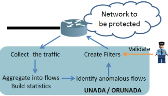
Fig. 1. Overall functionning of the detector
is set at the knee point value of the sorted curve. This value is computed with the knee point algorithm proposed in [27]. Every flow with a dissimilarity score above this threshold is considered as anomalous.
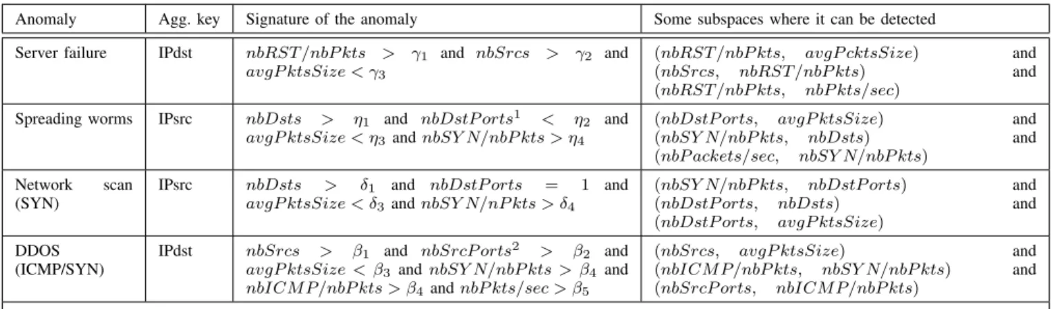
UNADA aims at detecting different types of anomalies which can be classified into two categories. The first category refers to network failures and performance problems like server or network failures, transient congestions, broadcast storms. The second category consists of network attacks like DOS, DDOS, worms. In Table I, every anomaly is described by a signature, i.e. by a set of inequalities that identifies a specific anomaly. It also specifies the level of aggregation used to get this signature and at least three subspaces where the anomaly may be spotted as an outlier. It displays a possible signature for a server failure. In our example, the server failure triggered a large number of RTS packets due to clients resetting their connection to the server. It also displays a signature for a DDOS attack made up of ICMP and SYN packets. Attackers often use different types of packets (here ICMP and SYN packets) during a DDOS to mitigate its detection.
Figure 1 displays a simple use of UNADA. UNADA is installed on the edge router of the network to be protected. It collects the traffic, aggregates it into flows and identifies anomalous flows. For each anomalous flow, UNADA specifies the value of its aggregation key which can be, for example, the IP source address of the anomaly if the aggregation key is IPsrc/32. The aggregation key value can then be used to filter the network and remove the anomalous flow: every packet matching the aggregation key may be discarded. The network administrator should give his approval before the removal of any anomalous flow as some of them may be legitimate like flash crowds. A flash crowd is an unusual burst of traffic to a single destination from a “typical” distribution of sources [19]. For example, a flash crowd may be induced by a temporal discount on a website. To reduce the network administrator task, UNADA provides for each anomalous flow its features and the subspaces where it is detected as an outlier.
UNADA detection performance has been extensively stud-ied with different public ground truths like the MAWILab [13], the METROSEC [18] and the KDD9 dataset [4], [5]. Evaluations showed that UNADA is able to detect a large fraction of attacks (at least 90% on every data set) with very
low false positive rates (less than 4%) and that it outper-forms the most commonly used approaches for unsupervised anomaly detection proposed in the literature: DBSCAN-based, K-means-based, and PCA-based outliers detection techniques [19], [20].
III. FEATURESPACEUPDATE WITH ADISCRETE
TIME-SLIDINGWINDOW
The detection is usually performed on network traffic col-lected in large time-slots implying long period of time between an anomaly occurrence and its detection. To overcome this issue, we propose to use a discrete time-sliding window in association with an unsupervised network anomaly detector. The proposed method is generic: any sufficiently fast and efficient detector can benefit from the proposed solution to reach continuous and real-time detection.
The traffic has to be collected in large time-slots of length ∆t in order to gather enough packets to catch flows patterns. Evaluations presented in [22] showed that UNADA detection performance is maximized with time-slots of 15 seconds, i.e. when ∆t = 15s. Collected traffic is then aggregated into flows with an aggregation key. Each flow is described by a set of features stored in a vector. These vectors are then concatenated in a normalized matrix X which represents the feature space. The network anomaly detection is then performed on the matrix X. The process of consecutive time-slots is illustrated in Figure 2.
To avoid that attacks damage the network, network anoma-lies have to be rapidly detected. To speed up the anomaly detection, we propose to update the feature space and launch the detection in a near continuous way, i.e. every micro-slot of length δt seconds.
However, if the feature space is computed with only the network traffic contained in a micro-slot, it may not contain enough information for the detectors to identify flows patterns and thus anomalies. To solve this issue, we use a discrete time-sliding window of length ∆t. The time window slides every micro-slot of length δt. When it slides, the feature space is updated. The feature space is the summary of the network traffic collected during the current time-window (see figure 3).
A discrete time-sliding window is made up of M micro-slots with M = d∆t/δte. To speed-up the feature space computation, the sliding window associates to each of its M micro-slots a micro-feature space mX. Each micro-feature space is computed with the packets contained in its micro-slot. The current window stores the M micro-feature spaces in a FIFO queue Q = (mX1, mX2, ..., mXM). mXM denotes
the micro-feature space computed with the packets contained in the newest micro-slot and mX1 in the oldest. When the
window slides a new feature space denoted Xnew can be
computed as follows:
Xnew= Xold+ mXnew− mX1 (1)
where Xold is the previous feature space and mXnew the
new micro-feature space. Finally, the FIFO queue is updated (mXnew is added to the FIFO queue and mX1 is removed),
TABLE I
FEATURES USED BYUNADAIN THE DETECTION OF SERVER FAILURE,NETWORK SCANS,SPREADING WORMS ANDDDOS. Anomaly Agg. key Signature of the anomaly Some subspaces where it can be detected Server failure IPdst nbRST /nbP kts > γ1 and nbSrcs > γ2 and
avgP ktsSize < γ3
(nbRST /nbP kts, avgP cktsSize) and (nbSrcs, nbRST /nbP kts) and (nbRST /nbP kts, nbP kts/sec)
Spreading worms IPsrc nbDsts > η1 and nbDstP orts1 < η2 and
avgP ktsSize < η3 and nbSY N/nbP kts > η4
(nbDstP orts, avgP ktsSize) and (nbSY N/nbP kts, nbDsts) and (nbP ackets/sec, nbSY N/nbP kts)
Network scan (SYN)
IPsrc nbDsts > δ1 and nbDstP orts = 1 and
avgP ktsSize < δ3 and nbSY N/nP kts > δ4
(nbSY N/nbP kts, nbDstP orts) and (nbDstP orts, nbDsts) and (nbDstP orts, avgP ktsSize)
DDOS (ICMP/SYN)
IPdst nbSrcs > β1 and nbSrcP orts2 > β2 and
avgP ktsSize < β3 and nbSY N/nbP kts > β4 and
nbICM P /nbP kts > β4and nbP kts/sec > β5
(nbSrcs, avgP ktsSize) and (nbICM P /nbP kts, nbSY N/nbP kts) and (nbSrcP orts, nbICM P/nbP kts)
1. nbDstPorts: number of different destination ports 2. nbSrcPorts: number of different source ports
Fig. 2. Feature space computation at the end of each time-slot of ∆t seconds
Fig. 3. Feature space computation at the end of each micro-time-slot of δt seconds
and the detector is applied to the updated feature space Xnew.
Any fast detector that can process the feature space in less than δt seconds can take benefit from this discrete time-sliding window to detect continuously network anomalies. To benefit from these feature space updates, we devised a new detector ORUNADA capable of detecting in continuous anomalies while preserving UNADA detection performance.
IV. ORUNADA
To reach real-time detection, ORUNADA takes advantage of a grid and incremental clustering algorithm.
Grid clustering algorithms divide the space into consecutive rectangular units or cells and then place points on the grid thus formed. Instead of grouping directly points in clusters, grid clustering algorithms group dense cells, i.e. cells containing many points, to form clusters. As the number of cells is
significantly lower than the number of points, they are less complex than usual clustering algorithms which group points like DBSCAN and K-means.
The drawback is that grid clustering algorithms usually output coarser clusters. For example (see Figure 4), a grid algorithm may incorrectly classify a point as an outlier due to its cells sharp edges.
However, we assume that replacing DBSCAN by a grid algorithm has little impact on UNADA detection performance as anomalies are extreme outliers, i.e. outliers located far away from clusters.
Furthermore, we make the assumption that few points enter and leave the feature space from one micro-slot to another. As a consequence, the feature space changes little from one micro-feature space to another. This assumption seems realistic as few packets arrive in δt seconds. If the assumption holds, updating the feature space partition instead of re-computing it
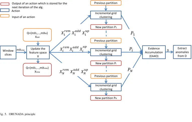
Window slices Update the feature space X Q=(mX1,…,mXM) Xold Incremental grid clustering Incremental grid clustering Incremental grid clustering Evidence Accumulation (EA4O) Previous partition Previous partition Extract anomalies from D
𝑋
1𝑟𝑟𝑟𝑋
1𝑎𝑎𝑎𝑋
1𝑢𝑢𝑋
𝑁𝑟𝑟𝑟𝑋
𝑁𝑎𝑎𝑎𝑋
𝑁𝑢𝑢𝑋
𝑖𝑟𝑟𝑟𝑋
𝑖𝑎𝑎𝑎𝑋
𝑖𝑢𝑢𝑃
1𝑃
𝑖𝑃
𝑁 mXnew Q=(mX2,…,mXnew) Xnew New partition P1 New partition Pi New partition PNOutput of an action which is stored for the next iteration of the alg.
Input of an action Action
D
Previous partition
Fig. 5. ORUNADA principle
Fig. 4. Output of a grid clustering algorithm. The point in red should belong to the cluster
entirely could save a significant amount of time.
Incremental clustering algorithms can update rapidly a fea-ture space partition when few points are added or removed. They take benefit from the fact that deleting or adding a point affect the current partition of the feature space only in the neighborhood of the point. Therefore, incremental clustering algorithms can efficiently update a feature space partition by re-computing only a few points.
Among available grid clustering algorithms, DGCA (Den-sity Grid-based Clustering Algorithm) [8] offers many ad-vantages; it can discover any shape of clusters and identify outliers. In DGCA, a group of consecutive dense cells forms a cluster. In the context of ORUNADA, we have slightly modified DGCA. We denote S = {A1 ∗ ... ∗ Ak} a
k-dimensional space where A1, ..., Ak are the dimensions of S.
Our modified version of GDCA takes as input a feature space X of size |F | ∗ k made up of k-dimensional points. DGCA
can be divided into four steps:
1) the space is divided into non-overlapping rectangular units or cells. The units are obtained by partitioning each dimension into intervals of size l. Each unit has the form u ={u1, .., uk} where ui = [li, hi) is a
right-open interval in the partitioning of Ai.
2) points are placed into the cells. Cells containing at least minDenseP ts are marked as dense units. A point x ={x1, ..., xk} belongs to a unit u ={u1, .., uk} if
li≤ xi≤ hi for all ui.
3) set of connected dense units are grouped together to form a cluster. Two k-dimensional dense units u1 and
u2 are connected if they have a common face or if
there exists another k-dimensional unit u3 such that u1
is connected to u3 and u2 is connected to u3. Units
u1 ={r1, ..., rk} and u2 ={r01, ..., r0k} have a common
face if there are k − 1 dimensions, assume A1, ..., Ak−1,
such that ri= r0ifor all i in [1, k − 1] and either hk = l0k
or h0k= lk.
4) it returns the clusters whose number of points is superior to minClusP ts
Points situated in cells which do not belong to any cluster are considered as outliers. Let n be the total number of points, c the number of cells, cn the number of non-empty cells, and
cd the number of dense cells, DGCA time complexity is then
O(n + cd.log(cn)). For the sake of comparison, DBSCAN
complexity is O(n2) and O(n.log(n)) when used with an R-tree index. Therefore, and as usually cd < cn c n holds,
There is an incremental version of GDCA called IDGCA (Incremental DGCA). IDGCA is able to update a feature space partition and, for a given input, outputs the same partition as DGCA.
IGDCA requires three input parameters (the same as GDCA): l the length used to divide each dimension into intervals, minDenseP ts the minimum number of points in a dense unit (or cell) and minClustP ts the minimum number of points to return a cluster. As in GDCA, the space is divided into non-overlapping rectangular units or cells. The units are obtained by partitioning each dimension into intervals of length li. At each feature space update, IDGCA upgrades
the previous partition. It takes as inputs the points to add Xadd, the points to remove Xremand the points to update Xupfrom
the previous partition. At each feature space update, IGDCA upgrades the previous partition in five steps:
1) for each point xup ∈ Xup, IDGCA identifies its new
unit unew and its previous unit uold (the unit to which
it belonged at the last update). If unewis different from
uold, IGDCA removes the point x from uold and adds
it to unew. It then removes every point xrem ∈ Xrem
from its unit and place every point xadd∈ Xaddinto its
unit.
2) it then computes two lists: the list of new dense units listN ewDenseU nits and the list of old dense units listOldDenseU nits. The first list contains the units which are now dense and were not dense in the previous partition. The second list contains the units which were dense in the previous partition and wich are not dense any longer.
3) every unit u in listOldDenseU nits is then processed and a list of units to re-partition listU nitT oRep is built. For each unit u ∈ listOldDenseU nits IDGCA removes u from the cluster C to which it belongs. If the unit u has two neighboring units which belong to the cluster C, then all the units of the cluster which are still dense are put in listU nitT oRep and the cluster is removed. Indeed, if the unit has two neighbors belonging to the cluster, its removal from the cluster may lead to a division of the cluster into two little clusters. Therefore all the units of the cluster which are still dense need to be re-partitioned. Once every unit in listOldDenseU nits has been processed, the dense units in listU nitT oRep are grouped to form clusters. Set of connected units forms a cluster.
4) every unit u in listN ewDenseU nits is processed. Each unit can either (1) form a new cluster (2) be absorbed by an existing cluster (3) or merge multiple clusters in one. If the unit u has no neighboring dense unit, IDGCA creates a new empty cluster to which it adds u. If the unit u has at least one dense neighboring unit and all its dense neighboring unit(s) belong to the same cluster, IDGCA adds u to this cluster. If the unit u has two or more neighboring dense units belonging to different clusters, IDGCA merges these clusters in one and adds u to this new cluster.
5) it returns the clusters whose number of points is superior
to minClusP ts. Points which do not belong to any of these clusters are considered as outliers.
Algorithm 1 ORUNADA Require:
the interval length l, min nb of pts in a dense unit minDenseP ts, min nb of pts in a cluster minClusP t, length slot ∆t and length micro-slot δt
Ensure:
list of anomalies listAnom
1: Initialize every partition P1, P2..., PN to null
2: Intialize IGDCA and slidingWindow
3: IGDCA.setP aram(l, minClusP ts, minDenseP ts) 4: slidingW indow.setP aram(∆t, δt)
5: nbU pdates = 0
6: while slidW indow.alive() do
7: if slidWindow. hasSlided() then
8: (Xrem, Xadd, Xup) = slidW indow.updateF S()
9: (Xrem, Xadd, Xup) = norm(Xrem, Xadd, Xup)
10: for i = 1 : N do
11: (Xirem, Xiadd, Xiup) = comp(Xrem, Xadd, Xup)
12: Pinew= IGDCA(Pi, Xirem, X add i , X up i ) 13: end for 14: nbUpdate++;
15: if nbU pdates ≥ d∆t/δte then
16: D = EA4O(P1new, ..., PNnew)
17: th = f indKneeP oint(D) 18: listAnom = extractAnomalies(D, th) 19: display(listAnom) 20: end if 21: end if 22: end while Algorithm 2 EA4O Require: the N Partitions P1, P2..., PN Ensure:
1: Initialize the dissimilarity vector D to null
2: for i = 1 : N do
3: center = getCenterBiggestCluster(Pi)
4: for outlier o in Pi.getOutliers() do
5: D(o) = D(o) + distance(o, center) 6: end for
7: end for 8: return sort(D)
ORUNADA takes advantage of both the discrete time-sliding window and the incremental grid clustering algorithm IDGCA. Algorithm 1 displays ORUNADA pseudo-code. First, ORUNADA initializes and sets the parameters of the in-cremental grid clustering algorithm and the discrete time-sliding window (line 1 to 4). ORUNADA is then made up of an infinite loop which is divided into three steps: the preprocessing step (line 8 and 9), the clustering step (line 10 to 14) and the anomalies extraction step (line 14 to 20). Every micro-slot, the window slides triggering the preprocessing step. During this step, the feature space X is updated and
the sliding window returns the points to remove Xrem, to add Xadd and to update Xup. These three matrices are then
normalized (line 9).
Next, the clustering step updates the partition of each subspace (line 10 to 14). It computes for each subspace the points to add Xiadd, to remove Xirem, and to update X
up i (line
11) and updates using IDGCA the previous subspace parti-tion Pi. For each subspace, IDGCA outputs a new partition
Pnew
i . The extraction step only occurs after d∆t/δte feature
space updates (line 15). During the first d∆t/δte − 1 feature space updates, the extraction step is not performed because the sliding window is not full, and ORUNADA may not have sufficient information on the network traffic to identify abnormal flows. This step combines the N obtained partitions using the EA algorithm for outliers identification (EA4O), and outputs a dissimilarity vector D (line 16). This dissimilarity vector associates to each flow a score of abnormality. A flow score is the cumulated sum of its distance to the center of the biggest cluster in every subspace where it is identified as an outlier (see Algorithm 2). Flows whose score is beyond a certain threshold are considered as anomalies. They are extracted using the function extractAnomalies (line 18). To set this threshold, the dissimilarity vector is sorted and plotted to obtain a curve. Normal flows possess low scores and form the tail of the curve. A change in the curve slope indicates a gap in the scores. This gap separates normal scores from abnormal ones. This change is represented by a knee point on the curve which can be used as a threshold. Its value can be easily computed with the knee point algorithm proposed in [27]. Finally, ORUNADA displays on the network administrator dashboard the set of anomalies using the display function (line 19). Figure 5 gives an overview of ORUNADA’s operation.
V. ORUNADA EVALUATION
UNADA has already been extensively evaluated on many data sets in [5] [4]. These studies have shown that UNADA reaches very good performance in terms of detection. Our study aims at answering the four following questions:
• By which factor DGCA improves UNADA execution time compared to DBSCAN?
• Does ORUNADA has the same detection performance as
UNADA-DBSCAN?
• What is the delay between an anomaly occurrence and
its detection?
• Is ORUNADA scalable with the traffic load?
ORUNADA is devised to run at the border link of the core network of a Spanish medium size Internet service provider. This link has to deal with a large amount of traffic: 300,000 packets/s and 1.2 Gbit/s on average. In the context of the ON-TIC project [1], the traffic crossing this link has been captured and anonymized since the beginning of 2014. For every packet, only the 64-bytes header is stored. The collected traffic forms the ONTS dataset and is available on demand for academic researchers. The ONTS access request form is available at the ONTIC project site [1]. To perform our validation, we use the file 20150210231651.pcap which contains 900 seconds of network traffic extracted the 10th of February 2015.
We use a second dataset: the MAWILab network traces. This dataset has been collected since 2001 until now. It consists of labeled 15 minutes network traces captured daily from a trans-Pacific link between Japan and the United States. This dataset is a ground truth and can be used to validate a detector performance in terms of true positive rate (TPR) and false positive rate (FPR). The labels were obtained by combining the results of four unsupervised network anomaly detectors [13].
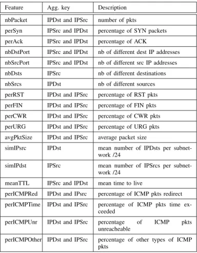
The evaluations are performed on a single machine with 16 GB of RAM and an Intel Core 5-4310U CPU 2.00GHz. In the following, the window size ∆t is set at 15 seconds, as UNADA obtained the best detection performance using this time window length (see [22]), and packets are aggregated into flows according to their IPsrc/32. We use at maximum 17 features to describe a flow. Table II provides the 20 flows features utilized for the evaluation, 17 can be obtained with the aggregation key IPsrc/32 and 17 with the aggregation key IPDst/32. The features can be modified according to the network administrator needs.
TABLE II FEATURES USED BYUNADA Feature Agg. key Description nbPacket IPDst and IPSrc number of pkts
perSyn IPSrc and IPDst percentage of SYN packets perAck IPSrc and IPDst percentage of ACK
nbDstPort IPSrc and IPDst nb of different dest IP addresses nbSrcPort IPSrc and IPDst nb of different src IP addresses nbDsts IPSrc nb of different destinations nbSrcs IPDst nb of different sources perRST IPDst and IPSrc percentage of RST pkts perFIN IPDst and IPSrc percentage of FIN pkts perCWR IPDst and IPSrc percentage of CWR pkts perURG IPDst and IPSrc percentage of URG pkts avgPktSize IPDst and IPSrc average packet size
simIPsrc IPDst mean number of IPDsts per subnet-work /24
simIPdst IPSrc mean number of IPSrcs per subnet-work /24
meanTTL IPSrc and IPDst mean time to live
perICMPRed IPDst and IPsrc percentage of ICMP pkts redirect perICMPTime IPDst and IPSrc percentage of ICMP pkts time
ex-ceeded
perICMPUnr IPDst and IPSrc percentage of ICMP pkts unreacheable
perICMPOther IPDst and IPSrc percentage of other types of ICMP pkts
For each dataset, we use the same methodology to set ORUNADA parameters. First, we aggregate into flows the traffic collected in a time window and remove the flows which have an extreme value in at least one dimension. We use the set of flows F thus formed, to set ORUNADA parameters. To normalize the feature space, we use the
max-Fig. 6. UNADA execution time
min normalization: for each dimension, the min is set at 0 and the max at the highest value for this feature in F . As we are looking for flows whose patterns significantly differ from the others, we do not need very accurate clusters. Therefore the length l of the interval in every dimension is set at 0.1, i.e. at 10% of the distance between the minimum and maximum value in every dimension in F . The minimum number of points minClusP ts in a cluster is set at 30% of the total number of flows in F . It implies that an anomaly cannot be detected if it is made up of more than minClusP ts flows. However, this is not an issue, as by using the appropriate aggregation level every anomaly can be summarized in one or few flows. The minimum number of points in a dense unit minDenseP ts is set at 5% of the total number of flows in F .
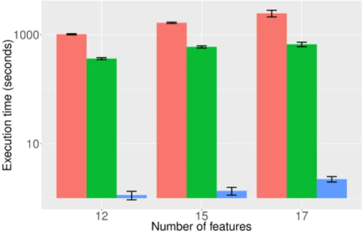
A. UNADA Execution time
ORUNADA needs to process quickly the incoming traffic to detect the anomalies efficiently. Therefore, we compared UNADA execution time using different clustering algorithms. Figure 6 depicts UNADA mean execution time (over 59 experiments) according to the clustering algorithm (DBSCAN, DBSCAN with an R*-tree [17] and DGCA) and the number of features (12, 15, 17) used. An R*-tree is a tree data structure used for indexing multi-dimensional information. An R*-tree can reduce DBSCAN execution time when it has to process a large feature space. The y-axis has a log-scale, so that the execution time of UNADA-DGCA can be observed and the error bar represents the standard deviation. UNADA-DGCA is in fact ORUNADA when ∆t = δt. The graph shows that DGCA improves the execution time of the detector. With 17 features, 15 seconds of traffic can be processed using UNADA-DGCA, on average, in two seconds.
Figure 7 confirms UNADA-DGCA performance. It displays the speed up factor of DGCA compared to UNADA-DBSCAN and UNADA-UNADA-DBSCAN with an R*-tree. One can notice that DGCA speeds up the execution time of UNADA by a factor of at least 300 compared to UNADA-R*-tree and 900 compared to UNADA-DBSCAN for 12, 15, and 17 features. Furthermore, ORUNADA could be further improved by distributing the computation of every subspace on a cluster of servers as proposed in [9].
B. Detection Similarity
This gain in execution time could negatively impact UN-ADA detection performance. To determine whether DGCA degrades UNADA’s detection performance, we compare the similarity of the anomalies found by UNADA-DGCA (i.e., ORUNADA with ∆t = δt) and UNADA-DBSCAN with different numbers of features (12, 15, 17). We use the Jaccard index (JI) to compare the set of anomalies found by these two detectors. This Jaccard index reflects the similarity between two sample sets. Let A be the first set and B the second set, the similarity between A and B according to the Jaccard index is computed as follows:
J (A, B) = |ASB|
|ATB| (2)
If the index is close to one, then the two sets are very similar, and if it is close to 0, then they are considered as very dissimilar. However, this index cannot provide any information about the degree of similarity between the anomalies rankings. Indeed, it could be interesting to determine if the anomalies with the highest dissimilarity scores are the same for both detectors as a network administrator will likely inspect them first. To evaluate the similarity between the detectors anomaly ranking we use a second similarity measure; the Spearman rank correlation coefficient (SC) [30]. Let two vectors X and Y of length n be two different rankings of n elements. Item i rank is denoted xi in X and yi in Y . The Spearman rank
correlation coefficient between these two vectors is computed as follows:
S(X, Y ) = 1 − 6 ∗P d
2 i
n(n2− 1) (3)
where di = xi − yi is the difference in rank for item
i. The rank of an anomaly depends on its position in the sorted dissimilarity vector D. The most dissimilar flow, i.e. the anomaly with the highest dissimilar value is ranked first. The second most dissimilar flow in the vector D is ranked second, etc. A Spearman rank correlation coefficient of 1 reflects a perfect similarity between the two rankings and a SC of -1, a complete dissimilarity. To point out the difference between
Fig. 8. Jaccard index between UNADA-DGCA and UNADA-DBSCAN outputs
the two clustering algorithms (DBSCAN and DGCA), we also compute the Jaccard index and the Spearman rank correlation coefficient for every flow detected as an outlier in at least one subspace.
Figure 8 displays the Jaccard index for the set of anomalies (in red) and outliers (in yellow) output by UNADA-DGCA and UNADA-DBSCAN with different numbers of features. In terms of anomalies, it can be noticed that the JI is equal to one which implies that DGCA and UNADA-DBSCAN find the same anomalies and have, therefore, the same detection performance. However, the JI in terms of outliers is low (0.58 for 12 features), meaning that they do not find the same outliers in every subspace and do not output the same partitions. Figure 9 confirms these results and displays the Spearman rank correlation coefficient between the anomalies and outliers ranking obtained by UNADA-DGCA and UNADA-DBSCAN. In terms of anomalies, the SC is equal to 1, which means that the detectors find the same anomalies and rank them in the same order. In terms of outliers, the SC is quite high (always superior to 0.83), therefore the detectors outliers rankings are quite similar. The above figures demonstrate that DGCA and
UNADA-Fig. 9. Spearman rank correlation coefficient between UNADA-DGCA and UNADA-DBSCAN outputs
Fig. 10. DBSCAN partition of a two-dimensional subspace
DBSCAN output the same anomalies with a similar ranking even though they generate different subspaces partitions. Thus, the evaluations show that DGCA can replace DBSCAN in UNADA with nearly no impact on the detection performance while improving its speed by a factor of at least 900.
Figures 10 and 11 display respectively DBSCAN and DGCA partitions of a two-dimensional subspace. The y-axis represents the percentage of RST packets, and the x-axis the percentage of SYN packets. DBSCAN and DGCA both find one big cluster which represents the set of normal flows. The differences between the two partitions are surrounded in Figure 11. UNADA-DGCA and UNADA-DBSCAN find the same five anomalies depicted by red circles. Three are related to this subspace: the two RST attacks and the SYN attack. The other two are classified as anomalies because they are extreme outliers in other subspaces.
Fig. 12. ORUNADA execution time according to the micro-slot length
C. ORUNADA Detection Frequency
The following evaluation aims at determining the smallest length of the micro-slot below which ORUNADA cannot be run online. The maximum frequency of ORUNADA detection is inversely proportional to this length. The smaller the micro-slot size, the faster ORUNADA identifies the anomalies and the network administrator takes countermeasures. Thus, we have evaluated ORUNADA execution time with different micro-slot sizes. The experiments have been performed using different numbers of features and the results are displayed in Figure 12. It can be noticed that a reduction of the micro-slot size improves ORUNADA average runtime. ORUNADA can process the incoming traffic faster than it arrives as long as the micro-slot size is superior or equal to 0.3 seconds (for 17 features) and 0.2 for (15 features).
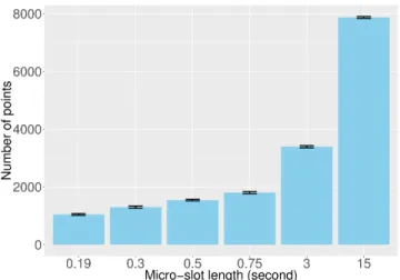
These results may be explained by the fact that few points are added, updated or removed from the feature space from one micro-slot to another (otherwise there would have been no gain in ORUNADA runtime with the decrease of the micro-slot size). Figure 13 confirms this assumption by displaying the average number of points that ORUNADA has to deal with each time the window slides according to the micro-slot length. It corresponds to the cumulated sum of the number of points to add, to remove and to update. This evaluation proves that ORUNADA can detect online with a low delay network anomalies (less than half a second elapses between an anomaly occurrence and its detection).
D. ORUNADA Scalability Performance
As IDGCA groups units instead of points, ORUNADA should scale well with the number of points (flows). To validate its scalability, we measured the execution time of ORUNADA using 9 different network traces from the MAW-ILab database. Every network trace lasts 15 minutes and was collected at various time periods between 2006 and 2015. Therefore, they exhibit different numbers of flows per time window of 15 seconds. Figure 14 displays the mean execution time of ORUNADA according to the average number of flows per time window for each network trace. These experiments were performed using a micro slot of 500 ms and 17 features
Fig. 13. Mean number of points to add, remove or update at each update of the feature space partition according to the size of the micro-slot length
Fig. 14. Mean execution time of ORUNADA according to the average number of flows using a micro-slot of 500 ms and 17 features
per flow. We can observe a linear relationship between the number of flows and ORUNADA execution time with an intercept of 42 and a slope of 0.04. This evaluation shows that ORUNADA has a linear relationship with the number of flows and can thus scale well with the traffic load.
The intercept low value indicates that the time dedicated to the partition of the units is very short (inferior to 42 ms). As explained in Section 1, two lists are generated to increment the feature space partition: the list of new dense units listN ewDenseU nits and the list of old dense units listOldDenseU nits. If there is no unit in these lists, the fea-ture space partition does not change. Furthermore, ORUNADA time complexity depends on the units in these lists. The short time dedicated to the partition of the units can be explained by a very small number of units in listN ewDenseU nits and listOldDenseU nits.
Figures 15 and 16 display the number of units in listN ewDenseU nits and in listOldDenseU nits at each feature space update using two different network traces: a MAWILab pcap file collected in 2015 (201501301400.dump) and an ONTS network trace collected in 2015 (20150210231651.pcap). Mots of the time the number of old dense units in both figures is hidden by the number
Fig. 15. Number of old and new dense units in time at every update of the feature space partition with the MAWILab dataset
Fig. 16. Number of old and new dense units in time at every update of the feature space partition with the ONTS dataset
of new dense units. In the first updates of the feature space partition, we can observe peaks in the number of new dense units. There are one large peak in the MAWILab network trace and one large peak followed by two smaller ones in the ONTS dataset. These peaks are linked to the creation of the feature space partition. Once the feature space partition is created, the number of new and old dense units remains very low and is most of the time null. These results reveal an important aspect on the nature of the network traffic used for these evaluations: flows features statistics are quite stable in time. Therefore, the network traffic feature space partition changes little over time. These two lists are both empty 86% percent of the time in the MAWILab network traces and 99.5% in the ONTS dataset. This study shows that the partition of the feature space is stable in time, which explains the low impact of the units partition upadte on ORUNADA execution time.
E. ORUNADA Detection Performance
UNADA detection performance has already been demon-strated via extensive studies in [4] and [5]. Furthermore, we have shown in subsection V-B that UNADA-DGCA (ORUNADA when ∆t = δt) and UNADA-DBSCAN detect the same anomalies and should then get the same detection performance. However, for completeness of this study, we validate ORUNADA on recent network traffic. As the ONTS dataset is not a ground-truth, the evaluations are performed with the MAWILab dataset. We use the 15 minutes traces collected the thirty of January 2015. These traces contain the
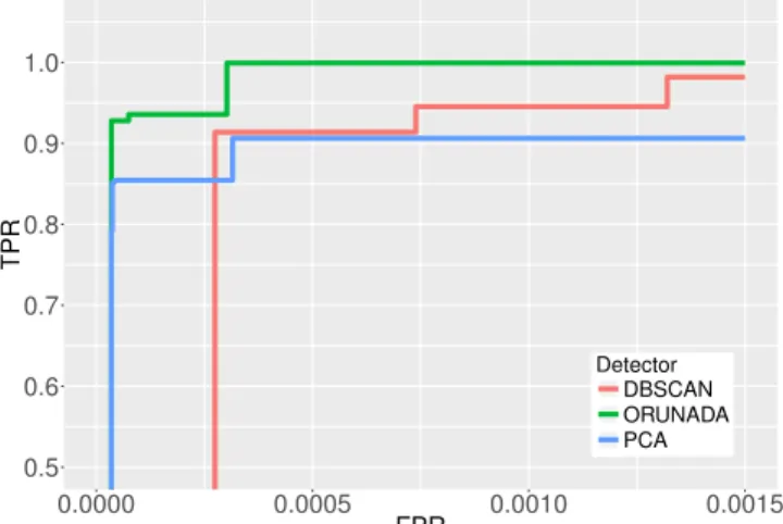
64 bytes-header of 130 M packets and 56 GB of network traffic. ORUNADA detection performance is compared with two detectors: a PCA-based [20] and a DBSCAN-based [31] detector. Figures 17 and 18 display the ROC curves obtained with different detectors using 17 features and the IPsrc/32 and the IPdst/32 aggregation flow key, respectively. To generate these curves, we vary the minimum number of points re-quired to form a cluster (for the DBSCAN-based detector and ORUNADA) and the number of principal component direc-tions of the abnormal subspace (for the PCA-based detector). These curves show that ORUNADA has a high detection rate with a low number of false positives and outperforms the other detectors. Its performance can be explained by the fact that it does not make any assumption on the data distribution unlike detection methods based on PCA and does not suffer from the curse of dimensionality like the DBSCAN-based detector. Indeed, the DBSCAN-based detector is sensitive to high dimensions because it processes the whole feature space directly and does not divide it into subspaces.
0.5 0.6 0.7 0.8 0.9 1.0 0.0000 0.0005 0.0010 0.0015 FPR TPR Detector DBSCAN ORUNADA PCA
Fig. 17. ROC curves with an aggregation flow performed at the IPsrc/32
0.5 0.6 0.7 0.8 0.9 1.0 0.000 0.001 0.002 0.003 FPR TPR Detector DBSCAN ORUNADA PCA
Fig. 18. ROC curves with an aggregation flow performed at the IPdst/32
VI. RELATEDWORKS
There are two main types of network anomaly detectors: supervised and unsupervised network anomaly detectors. Su-pervised network anomaly detectors rely on labels to learn a
Detector Technique(s) Advantage(s) Drawback(s)
[21] Grid clustering Reduce time complexity Low detection frequency [10] Association rule learning Generate clear signatures to describe
anomalies
(1) Use sampled traffic (2) High complexity [21] One class SVM (1) Adaptive to the operator feedback (2)
Give a confidence level for every anomaly
(1) High complexity (2) Suffer from the curse of dimensionality
[20] PCA Low false alarm rate Identify only points in time where anoma-lies occur
[28] PCA Solve PCA scalability issues Detect only volume anomalies [6] ARMA (1) Predict anomaly occurrence (2)
Visual-ization method of the anomalies
Identify only points in time where anoma-lies occur
[32] ARMA and an abrupt changes de-tection technique
Synthesize information from multiple met-rics
Assume that the traffic variables are quasi stationary
[7] Hadoop Generic framework for unsupervised net-work anomaly detectors
Require a large cluster of servers TABLE III
COMPARISON OF UNSUPERVISED NETWORK ANOMALY DETECTION SOLUTIONS
model for normal and abnormal traffic. These techniques suffer from two main issues: they are unable to adapt to new normal traffic and new types of anomalies. In contrast, unsupervised network anomaly detectors do not rely on any training data or prior knowledge. Therefore, they do not require any human input to build signatures, traffic profiles or to put labels on network traffic. They also have the ability to detect 0-day attacks. They rely on the assumption that anomalous traffic is rare and has different patterns from normal traffic. If the assumption does not hold, they may suffer from a high false alarm. However, by selecting an appropriate aggregation key to aggregate the traffic, the previous assumption might always be respected. In the literature, different techniques are used to detect network anomalies in an unsupervised way; machine learning techniques (clustering algorithm [26], [21], [23], outlier detection algorithms, Support Vector Machines (SVM)) [14], statistical techniques (Gaussian mixture model [15], histograms [16], Principal Component Analysis (PCA) [19]) and signal processing techniques (Auto-Regressive and Moving Average (ARMA) method [6] [32], change detection method [32]). Table III summarizes the techniques, advan-tages and drawbacks of some existing unsupervised network anomaly detection solutions.
In [21], Leung et al. propose a new density and grid-based clustering algorithm that is suitable for unsupervised network anomaly detection. It decreases the time complexity of usual clustering using histograms and frequent pattern tree. However, their solution is still exponential with the number of dimensions and quadratic in the number of clusters. Furthermore, the feature space partition has to be entirely re-computed at each time-slot.
In [10], the authors propose an unsupervised network anomaly detector based on an outlier detection algorithm which uses association rules for summarizing anomalous flows. Their solution shows promising results to detect and generate clear signatures for every anomaly. However, due the high complexity of their algorithm (quadratic with the number of flows), they use a sampled traffic. Sampling may have a negative impact on the detection performance: the detector
may not have enough information to take accurate decisions. In [14], the authors propose an online and adaptive anomaly detection system based on a one-class SVM. This one-class SVM computes a hyperplane with unlabeled training data. This hyperplane identifies a small region of the feature space that contains most of the vectors. Normal flows are supposed to be located in this small region. Future input vectors are classified based on their relationship to the hyperplane. Their solution provides several interesting properties: it can handle dynamic input normalization, adapt the detection to the feedback of the operator and determine for each detected anomaly a level of confidence. The authors claim that their solution can be used online, however, computing the hyperplane is a very complex task performed in O(n3) in the worst case with n the number of flows. Furthermore, the hyperplane has to be recomputed each time the operator feedback is in contradiction with the detector output. SVM also suffers from the curse of dimensionality [12], [2] and is, therefore, limited in the number of features it can use (they use three features per flow in the article). A low number of features may have a negative impact on the detection performance of the solution.
Detectors based on PCA divides the whole space into two subspaces. The first k principal component (PC) directions of the data matrix are used to construct the normal subspace and the remaining PC directions to build the abnormal subspace. Points with a large norm in the abnormal subspace deviate from the normal subspace and are, therefore, identified as outliers. Many network anomaly detectors has successfully applied PCA [29], [19], but the work of Lakhina et al, published in [19] is one of the most exhaustive. However, and as mentioned in [24], PCA-based detectors consider that the data follows a jointly Gaussian distribution which may be unrealistic in the case of network traffic. This assumption allows them to apply the Q-statistic to set the threshold used to detect the anomalies. This threshold guarantees a theoretical bound for the FPR.
Lakhina et al. [19] propose a PCA-based detector to detect anomalies on multiple time-series and use entropy to capture features distribution and improve detection. Their evaluation
shows good results. However, their solution can identify the points in time where an anomaly occurs but is unable to identify the flow(s) which trigger(s) the alert.
In [28], Schölkopf et al. propose a solution to overcome the scalability problem of PCA-based anomaly detectors. To solve this issue they use an adaptive local data filter which sends to a coordinator just enough data to enable accurate global detection. The coordinator applies then the PCA-based anomaly detector as proposed by Lakhina et al. Their solution aims at detecting only volume anomalies, as a result, it cannot detect many interesting anomalies like network or port scans, ping of the death, and teardrops.
Some unsupervised machine learning techniques use time series and signal processing techniques to identify anomalies. These systems usually only detect the point in time where an anomaly occurs and are unable to detect the flows responsible of an anomaly. After an anomaly detection the network ad-ministrator has to examine the data manually to identify the flow(s) which trigger(s) the anomaly.
In [6], Celenk et al. propose a method to visualize and predict network anomalies. Their solution collects statistics on the incoming traffic in consecutive time windows. It computes for each statistic its entropy and its fisher linear discriminant (FLD) performance index. A high FLD indicates a network anomaly. They consider that every attack is preceded by an initialization phase, therefore, their solution can predict an attack by identifying its initialization phase. They apply a Wiener filter and an Auto-regressive moving average model on the traffic statistics to forecast anomalies. Their solution can predict when an anomaly occurs, however, it is unable to identify the flow(s) responsible for the anomaly.
In [32], Thottan et al. present a network anomaly detection method based on signal processing techniques and abrupt changes and allow to synthesize information from multiple metrics. They apply their solution on time series of MIB variables. Each time series is described by an ARMA model. It detects changes in time series using a hypothesis test on the generalized likelihood ratio (GLR). Each GLR outputs an abnormality vector which is then combined using a linear operator. However, the authors assume that the traffic variables are quasi stationary. This strong assumption has not yet, to our knowledge, been proven or demonstrate. Furthermore, as the network traffic evolves in time, this assumption may seem unrealistic.
The solutions presented above are offline detectors which do not consider time and scalability. There exist few solutions which tackle these issues. One of them is Hashdoop [7]. Hashdoop is a generic framework which aims at speeding up any unsupervised network anomaly detector. To do so, it launches many instances of the detector in parrallel on a cluster of servers using the distributed computing framework MapReduce of Hadoop [7]. To distribute the traffic while respecting detectors requirements, the authors propose to dis-tribute the incoming network traces in such a way that the traffic spatial and temporal structure is preserved. The authors claim that their solution allows speeding up any network anomaly detector. However, their solution requires a large cluster of servers, and few firms can afford dedicating a cluster
of servers for network anomaly detection.
Our solution solves the issues pointed out in the articles described above:
• it solves the curse of dimensionality by using subspaces and evidence accumulation techniques. Therefore, it can deal with high dimensions whereas [14] is limited in the number of dimensions as it suffers from the curse.
• it detects when an anomaly occurs and identifies the flows
responsible. Solutions presented in [32], [6] and [19] can only detect the points in time where an anomaly occurs.
• it does not make any assumption on the normal network traffic model. PCA-based detectors presented in [19] and [28] consider that normal network traffic follows a mul-tivariate Gaussian distribution. However, this assumption may not always be true and, to our knowledge, has never been proven.
• it detects many types of anomalies. Some detectors detect only volume anomalies [28], as a consequence, they cannot identify subtle anomalies like scans, pings of the death, and smurfs.
• it has a low complexity. Network anomaly detectors often
suffer from a high complexity like [14] and [10]. As shown in our experiments, the time complexity of our solution is nearly linear with the number of flows as the feature space partition remains stable in time. Therefore, it can detect network anomalies online and on a single machine.
VII. CONCLUSION ANDFUTUREWORKS
ORUNADA is a scalable and real-time unsupervised net-work anomaly detector. It relies on a discrete time-sliding window to process in continuous the incoming traffic and on an incremental grid clustering to update the feature space partition. It detects, with a low delay, network anomalies in order to remove them before they damage the network.
ORUNADA collects the network traffic at the border link of the network to be protected using a discrete time sliding window. The traffic is then aggregated into flows. Flows are described by a large set of features. To overcome the curse of dimensionality, the feature space is divided into subspaces. A clustering algorithm is then performed on each subspace to detect outliers. To speed up the clustering step, ORUNADA relies on a grid and incremental clustering algorithm which updates every partition instead of recomputing them. The obtained partitions are then merged to identify the most dissimilar outliers and thus, the anomalies. Our discrete time-sliding window is generic and can be used by any fast detector to detect anomalies in a continuous way.
Our evaluation shows that ORUNADA is scalable with the number of flows and can be used online to detect anomalies with a low delay and good detection performance. The results demonstrate that the use of a grid clustering algorithm speeds up by a factor of at least 900 ORUNADA. They also show that the subspace partition is stable in time, as a consequence, the execution time of ORUNADA is nearly always linear with the number of flows. The evaluations demonstrate that ORUNADA can detect on the core network of an intermediate
size Internet service provider, anomalies in less than half a second after their occurrence, using 17 features. Furthermore, our solution offers similar detection performance in terms of TPR and FPR to UNADA.
To further improve its speed, we have planned to distribute its computation over a cluster of servers using tools from the Big Data world such as Spark Streaming. Spark Streaming is a framework for distributing the computation of algorithms which have, as input, very large stream of data. Moreover, we would like to integrate the feedback of the network adminis-trator to refine the detection performance of our solution.
ACKNOWLEDGMENT
The research leading to these results has received funding from the European Union Seventh Framework Programme (FP7/2007-2013) under grant agreement n°619633 (Collabo-rative project ONTIC).
REFERENCES
[1] Online network traffic characterization. http://ict-ontic.eu/, 2014. Ac-cessed: 2016-02-18.
[2] Y. Bengio, O. Delalleau, and N. Le Roux. The curse of highly variable functions for local kernel machines. In Proc. of the 18th Int. Conf. on Neural Information Processing Systems, pages 107–114, Cambridge, MA, USA, 2005. MIT Press.
[3] D. Brauckhoff, B. Tellenbach, A. Wagner, M. May, and A. Lakhina. Impact of packet sampling on anomaly detection metrics. In ACM SIGCOMM Conf. on Internet Measurement, pages 159–164. ACM, 2006.
[4] P. Casas, J. Mazel, and P. Owezarski. NETWORKING 2011: 10th Int. IFIP TC 6 Networking Conf., chapter UNADA: Unsupervised Network Anomaly Detection Using Sub-space Outliers Ranking, pages 40–51. Springer Berlin Heidelberg, 2011.
[5] P. Casas, J. Mazel, and P. Owezarski. Unsupervised network intrusion detection systems: Detecting the unknown without knowledge. Comput. Comm., 35(7):772 – 783, 2012.
[6] M. Celenk, T. Conley, and J. Willis, J.and Graham. Predictive network anomaly detection and visualization. IEEE Trans. Inf. Forensics Security, 5(2):288–299, Jun 2010.
[7] J. Chen, R. Fontugne, A. Kato, and K. Fukuda. Clustering spam campaigns with fuzzy hashing. In AINTEC Asian Internet Eng. Conf., page 66, Febr. 2014.
[8] N. Chen, A. Chen, and L. Zhou. An incremental grid density-based clustering algorithm. Journal of Software, 13(1), Aug. 2002.
[9] J. Dromard, G. Roudière, and P. Owezarski. Unsupervised Network Anomaly Detection in Real-Time on Big Data. In New Trends in Databases and Information Systems, volume 539, pages 197–206. Springer, 2015.
[10] L. Ertoz, E. Eilertson, A. Lazarevic, P. Tan, J. Srivastava, V. Kumar, and P. Dokas. The MINDS - Minnesota Intrusion Detection System. In Next Generation Data Mining. MIT Press, 2004.
[11] M. Ester, H-P. Kriegel, J. Sander, and X. Xu. A density-based algorithm for discovering clusters in large spatial databases with noise. In Proc. of the Second Int. Conf. on Knowledge Discovery and Data Mining, pages 226–231, 1996.
[12] P. F. Evangelista, M. J. Embrechts, and B. K. Szymanski. Taming the Curse of Dimensionality in Kernels and Novelty Detection, pages 425– 438. Springer Berlin Heidelberg, Berlin, Heidelberg, 2006.
[13] R. Fontugne, P. Borgnat, P. Abry, and K. Fukuda. MAWILab: Combining Diverse Anomaly Detectors for Automated Anomaly Labeling and Performance Benchmarking. In ACM CoNEXT ’10, Philadelphia, PA, 2010.
[14] D. Ippoliti and X. Zhou. Online adaptive anomaly detection for augmented network flows. In IEEE 22nd Int. Symp. on Modelling, Analysis Simulation of Comput. and Telecommun. Syst., pages 433–442, Sept. 2014.
[15] M. Khaleghi and M. Bahrololum. Anomaly intrusion detection system using gaussian mixture model. Int. Conf. on Convergence Inform. Technol., 01:1162–1167, 2008.
[16] A. Kind, M.P. Stoecklin, and X. Dimitropoulos. Histogram-based traffic anomaly detection. IEEE Trans. on Network and Service Management, 6(2):110–121, June 2009.
[17] H-P. Kriegel, R. Schneider, B. Seeger, and N. Beckmann. The R*-tree: an efficient and robust access method for points and rectangles. Sigmod Record, 19:322–331, 1990.
[18] LAAS-CNRS. Metrology for security and quality of service. http: //projects.laas.fr/METROSEC/. Accessed: 2016-02-18.
[19] A. Lakhina and M. Crovella. Mining anomalies using traffic fea-ture distributions. ACM SIGCOMM Comput. Communication Review, 35(4):217, 2005.
[20] A. Lakhina, M. Crovella, and C. Diot. Diagnosing network-wide traffic anomalies. In Conf. on Applications, Technologies, Architectures, and Protocols for Comput. Commun., pages 219–230, New York, NY, USA, 2004. ACM.
[21] K. Leung and C. Leckie. Unsupervised anomaly detection in network in-trusion detection using clusters. In Twenty-Eighth Australasian Comput. Science Conf. (ACSC2005), pages 333–342, 2005.
[22] J. Mazel. Unsupervised network anomaly detection. PhD thesis, INSA, France, Dec. 2011.
[23] A. P. Muniyandi, R. Rajeswari, and R. Rajaram. Network anomaly de-tection by cascading k-means clustering and c4.5 decision tree algorithm. Procedia Engineering, 30:174 – 182, 2012.
[24] J. Ndong and K. Salamatian. Signal Processing-based Anomaly Detec-tion Techniques: A Comparative Analysis. In INTERNET 2011, pages 32–39, Luxembourg, 2011.
[25] A. Patcha and J. Park. An overview of anomaly detection techniques: Existing solutions and latest technological trends. Comput. Netw., 51(12), Aug 2007.
[26] L. Portnoy, E. Eskin, and S. Stolfo. Intrusion detection with unlabeled data using clustering. In Proc. of ACM CSS Workshop on Data Mining Applied to Security (DMSA), 2001.
[27] V. Satopaa, J. Albrecht, D. Irwin, and B. Raghavan. Finding a “kneedle” in a haystack: Detecting knee points in system behavior. In International Conf. on Distributed Computing Systems Workshops, pages 166–171, Minneapolis, Minnesota, USA, 2011.
[28] B. Schökopf, J. Platt, and T. Hofmann. In-Network PCA and Anomaly Detection, pages 617–624. MIT Press, 2007.
[29] M-L Shyu, S-C Chen, K. Sarinnapakorn, and L. Chang. A novel anomaly detection scheme based on principal component classifier. In IEEE Foundations and New Directions of Data Mining Workshop, pages 171– 179, 2003.
[30] C. Spearman. The proof and measurement of association between two things. The American Journal of Psychology, 15(1):72–101, 1904. [31] T. M. Thang and J. Kim. The anomaly detection by using dbscan
cluster-ing with multiple parameters. In Information Science and Applications (ICISA), pages 1–5, April 2011.
[32] M. Thottan and Chuanyi Ji. Anomaly detection in ip networks. IEEE Trans. Signal Process., 51(8):2191–2204, Aug 2003.
Juliette Dromard has received her engineering de-gree in 2010 in Information and Telecommunica-tion Systems from the University of Technology of Troyes (UTT). In 2013, she got a doctor’s degree in Network, Knowledge and Organization from UTT for her thesis entitled Towards a secure admission control in a wireless mesh networks. She is currently in post-Doctoral position in LAAS-CNRS. Her re-search interests are in the areas of unsupervised network anomaly detection, unsupervised machine learning techniques, big data mesh networks and admission control.
Gilles Roudiere is a PhD student working at the LAAS (Laboratory for Analysis and Architecture of Systems), in Toulouse, France. As a computer science graduate from the INSA (National Institute of Applied Science) of Toulouse, he started his PhD in 2015. As his field of research relates to Internet security issues, he is currently working on building a new network anomaly detector that provides a more autonomous detection. His researches lead him to investigate techniques that are able to deal with networks big data, such as machine learning and data mining.
Philippe Owezarski is director of research at CNRS (the French center for scientific research), working at LAAS (Laboratory for Analysis and Architecture of Systems), in Toulouse, France. He got a PhD in computer science in 1996 from Paul Sabatier University, Toulouse III, and an habilitation for ad-vising research in 2006. His main interests deal with next generation Internet. More specifically Philippe Owezarski takes advantage of IP networks monitor-ing for enforcmonitor-ing Quality of Service and security. It especially focuses on techniques as machine learning and data mining on the big data collected from the networks for making the network related analytics autonomous and cognitive.