HAL Id: hal-01472577
https://hal.archives-ouvertes.fr/hal-01472577v2
Preprint submitted on 2 Mar 2017
HAL is a multi-disciplinary open access
archive for the deposit and dissemination of sci-entific research documents, whether they are pub-lished or not. The documents may come from teaching and research institutions in France or
L’archive ouverte pluridisciplinaire HAL, est destinée au dépôt et à la diffusion de documents scientifiques de niveau recherche, publiés ou non, émanant des établissements d’enseignement et de recherche français ou étrangers, des laboratoires
Fixed Point Solution to Stochastic Priority Games
Bruno Karelovic, Wieslaw Zielonka
To cite this version:
Bruno Karelovic, Wieslaw Zielonka. Fixed Point Solution to Stochastic Priority Games. 2017. �hal-01472577v2�
Fixed Point Solution to Stochastic Priority Games
Bruno Karelovi´c and Wies law Zielonka IRIF, Universit´e Paris Diderot - Paris 7 case 7014, 75205 Paris Cedex 13, France
[email protected] [email protected]
March 1, 2017
Abstract
We define and examine a class of two-player stochastic games that we call priority games. The priority games contain as proper subclasses the parity games studied in computer science [4] and the games with the limsup and liminf payoff mappings. We show that the value of the priority game can be expressed as an appropriate nested fixed point of the value mapping of the one-day game. This extends the result of de Alfaro and Majumdar [4], where the authors proved that the value of the stochastic parity game can be expressed as the nested fixed point of the one-day value mapping.
The difference between our paper and [4] is two-fold.
The value of the parity game is obtained by applying the least and the greatest fixed points to the value mapping of the one-day game. However, in general, the greatest and the least fixed-points are not sufficient in order to obtain the value of the priority game.
To cope with this problem we introduce the notion of the nearest fixed point of a monotone bounded nonexpansive mapping. Our main result is that the value of the priority game can be obtained as the nested nearest fixed point of the value mapping of the one-day game.
The second point that makes our proof different from [4] is that our proof is inductive. We give a game interpretation for the nested fixed point formula where some variables are free (not bounded by the fixed point operator). Thus instead of proving the main result in one big step as in [4] we can limit ourselves to the case when just one fixed point is added to the nested fixed point formula.
1
Introduction
Stochastic two-player zero-sum games model the long-term interactions between two players that have strictly opposite objectives.
The study of stochastic games starts with the seminal paper of Shapley [10]. Since then stochastic games were intensively studied in game theory and, more recently, in computer science.
In stochastic games players’ preferences are expressed by means of a payoff mapping. The payoff mapping maps infinite plays (infinite sequences of states and actions) to real numbers. The payoff mappings used in computer science tend to be different from the payoff mappings used in game theory. The payoffs prevalent in computer science are often expressed in some kind of logic which implies that they take only two values, 1 for the winning plays and 0 for the losing plays.
On the other hand, the payoff mappings used in game theory are rather real valued: mean-payoff, discounted payoff, lim sup and lim inf payoffs are among the most popular ones.
In this paper we define and examine the class of priority games. The priority games constitute a natural extension of parity games, this latter class is the class of games popular in computer science having applications in automata theory and verification.
However, the priority games are also relevant to the games traditionally studied in game theory. It turns out that the games with the limsup and liminf payoff [8] belong to the class of priority games.
To put the results of the paper in the context we recall below the relevant results concerning the stochastic parity games due to deAlfaro and Majumdar [4].
1.1 Parity games
A stochastic parity game is a zero-sum two-player game infinite game played by two players, player Max and player Min, on an arena with a finite set of states S “ rns “ t1, . . . , nu.
For each state i, players Max and Min have nonempty sets of available actions, Apiq and Bpiq respectively. At each stage, the players, knowing the current state and all the previous history, choose independently and simultaneously actions a P Apiq and b P Bpiq respectively and the game moves to state j with probability ppj|i, a, bq. Immediately after each stage, and before the next one, both players are informed about the action played by the adversary player.
An infinite sequence of states and action occurring during the game is called a play. The parity games are endowed with the reward vector r “ pr1, . . . , rnq, where ri P
t0, 1u is the reward of state i. The parity payoff ϕphq of an infinite play h is defined to be equal1 to the reward of the maximal state visited infinitely often in h, i.e. the payoff
is equal to ri if i was visited infinitely often in h and all states j, j ą i, were visited only
a finite number of times.
The set of all plays is endowed in the usual way with the Borel σ-algebra generated by the cylinders. Strategies σ, τ of players Max and Min and an initial state i P S give rise to a probability measure Pσ,τi over the Borel σ-algebra. The aim of player Max (respectively Min) is to maximize (respectively minimize) the expected payoff
Eσ,τi pϕq “ ż
ϕphqPσ,τi pdhq
1
The payoff of the parity game is usually formulated in a bit different way, however it is easy to see that the definition given here is equivalent to the usual one.
for each initial state i.
Since the parity payoff is Borel measurable, by the result of Martin [9], parity games have value vi for each initial state i, i.e.
sup σ inf τ E σ,τ i pϕq “ vi“ infτ sup σ Eσ,τi pϕq, @i P S. (1)
One of the techniques used to solve parity games relies on the µ-calculus. In this approach the point of departure is the one-day game2 played at each state i P S. The
one-day game has a value for each state i P S and each reward vector r “ pr1, . . . , rnq.
Let
f “ pf1, . . . , fnq (2)
be the mapping that maps the reward vector r P t0, 1un to the vector of values of the
one-day game, i.e. for r “ pr1, . . . , rnq and i P S, fiprq is the value of the one-day game
played at state i when the reward vector is r. We endow r0, 1sn with the product order,
x “ px1, . . . , xnq ď py1, . . . , ynq “ y if xi ď yi for all i P rns, which makes it a complete
lattice. It is easy to see that
f : r0, 1snÑ r0, 1sn
is monotone under ď, thus by Tarski’s theorem [11], f has the least and the greatest fixed points.
Then one can define the nested fixed point Fixnpf qprq “ µrnx
n.µrn´1xn´1. . . . µr2x2.µr1x1.f px1, x2, . . . , xn´1, xnq, (3)
where µrix
i denotes either the greatest fixed point if ri “ 1, or the least fixed point if
ri “ 0, and f the value function (2) of the one-day game. The main result obtained by
de Alfaro and Majumdar [4] in the µ-calculus approach to parity games is that
v “ pv1, . . . , vnq “ Fixnpf qprq,
where the left-hand side vector v is composed of the values vi for the parity game starting
at i, cf. (1). To summarize, the value vector of the parity game can be obtained by calculating the nested fixed point of the one-day value mapping3.
The µ-calculus approach to parity games was first developed for deterministic parity games (perfect information games with deterministic transitions), see Walukiewicz [12]. The paper of de Alfaro and Majumdar [4] extended this approach to stochastic parity games.
2
In computer science papers the one-day game is often not mentioned explicitly, but the value function f of the one-day game is used in the µ-calculus approach to parity games, where it is sometimes called the predecessor operator.
3
The traditional presentation of this result is a bit different. Roughly speaking the variables are regrouped in blocks, each block consists of consecutive variables to which the same fixed point is applied. The each fixed point is applied to a group of variables rather than to separate variables. This allows to decreases the number of fixed points and the resulting formula alternates the least and the greatest fixed points. This is, however, only a technical detail which has no bearing on the result. For our purposes it is more convenient to apply fixed points to variables rather than to groups of variables.
1.2 From parity games to priority games
The parity games arose from the study of decidability questions in logic. In this frame-work the winning criteria are expressed in some kind of logic, where there is room for only two types of plays, the winning plays that satisfy a logical formula and the losing plays that do not satisfy the formula. For this reason the rewards in the parity games take only two values, 0 and 1, with the intuition that the reward 1 is favorable and the reward 0 unfavorable for our player (and the preferences are inverse for the adversary player).
However, the restriction to 0, 1 rewards does not allow to express finer player’s preferences. This motivates the study of the games that allow any real rewards.
We define the priority game as the game where each state i P rns “ S is equipped with a reward ri P R. Like in the parity game the payoff ϕphq of a play h is defined to
be the reward ri of the greatest state i that is visited infinitely often in h.
At first glance, the priority game is just a mild extension of the parity game. This impression is reinforced by the fact that deterministic priority games can be reduced to deterministic parity games. (However, we do not know if such reduction is possible for stochastic priority games.)
The interest in priority games is twofold. First, the priority games allow to quantify players’ preferences in a more subtle way than it is possible in parity games. While in parity games there are only two classes of plays, the plays with the parity payoff 1 and the plays with the parity payoff 0, in priority games we can distinguish many levels of preferences. As a motivating simple example consider the priority game with three states S “ t1, 2, 3u and rewards r1 “ 0, r2 “ 1, r3 “ 34. This game gives rise to three
distinct classes of infinite plays: player Max highest preference is for the plays such that the maximal state visited infinitely often is state 2 (these plays give him the payoff 1), his second preference is for the plays that visit state 3 infinitely often (such plays give him the payoff 34), and his lowest preference is for the plays that from some moment onward stay forever in state 1 (this yields him the payoff 0). It is impossible to capture such a hierarchy of preferences when we limit ourselves to the parity payoff.
The second reason to be interested in the games with priority payoff stems from the fact that not only they generalize the parity games, but they contain as proper subclasses the games with the lim sup and lim inf payoffs [7]. Let pikq8k“1 be the infinite sequence
of states visited during the play, where ik is the state visited at stage k. Let prikq
8 k“1 be
the corresponding sequence of rewards. The limsup game (respectively liminf game) is the game with the payoff equal to lim supkrik (respectively lim infkrik).
To see that a limsup game is a priority game let us take a finite state limsup game and rename the states in such a way that for any two states i, j P rns, if i ă j then ri ď rj, i.e. the natural order of states reflects the reward order. Then the limsup payoff
will be equal to the priority payoff.
For a liminf game we proceed in a similar way: we rename the states in such a way that, for any two states i, j P rns, i ă j implies that rj ď ri. Under this condition the
liminf payoff will be equal to the priority payoff.
games. There are two major differences however.
It is impossible to solve the priority games using only the least and the greatest fixed points, we need also other fixed points that we name “the nearest fixed points”. To define this notion we use the well known fact that the one-day game value mapping (2) is not only monotone but it is also nonexpansive, which means that, for x, y P Rn,
kfpxq ´ fpyqk8 ďkx ´ yk8, wherekxk8 “ supi|xi| is the supremum norm.
In the study of parity games the fact that the one-day game value mapping f is nonexpansive is irrelevant, the monotonicity of f is all that we need in order to apply Tarski’s fixed point theorem. When we study the priority games, other fixed points enter into consideration and the fact that f is nonexpansive becomes paramount.
It turns out that the priority games with rewards in R can be reduced through a linear transformation to the priority games with rewards in the interval r0, 1s. Therefore in the sequel we assume that the reward vector r “ pr1, . . . , rnq belongs to r0, 1sn. Under
this condition value mapping f of the one-day game (2) is a monotone nonexpansive mapping from r0, 1snto r0, 1sn. Since our study of priority games is based on the analysis
of the fixed points of f , in Section3 we prepare the background and present basic facts concerning fixed points of monotone nonexpansive mappings from r0, 1sn to r0, 1sn. All
the results presented in Section 3 are either well known or are rather straightforward observations. The only purpose of Section 3 is to regroup in one place all the relevant facts and to introduce the notion of the nearest fixed point
µrx.gpxq
of monotone nonexpansive mappings g : r0, 1s Ñ r0, 1s. Intuitively, µrx.gpxq is the fixed
point of g which is nearest to r P r0, 1s. Note that the least and the greatest fixed points of g are special cases of this notion, the greatest fixed point is the fixed point nearest to 1 and the least fixed point is the fixed point nearest to 0. We show that the notion of the nearest fixed point makes sense for monotone nonexpansive mappings from r0, 1s to r0, 1s. In Section 3 we define also, for each vector r “ pr1, . . . , rnq P r0, 1sn and a
monotone nonexpansive mapping f : r0, 1snÑ r0, 1sn, the nested nearest fixed point
Fixnpf qprq “ µrnx
n.µrn´1xn´1. . . . µr2x2.µr1x1.f px1, x2, . . . , xn´1, xnq, (4)
which generalizes the nested least/greatest fixed point (3). Section 4introduces the one-day games.
Section 5constitutes the core of the paper.
We prove that the value vector v “ pv1, . . . , vnq, where vi is the value of state i in
the priority games satisfies
v “ pv1, . . . , vnq “ Fixnpf qprq,
where the right-hand side is the nested nearest fixed point (4) of the value mapping of the one-day game.
Although the result of Section 5can be seen as an extension of the µ-calculus char-acterization known for parity games [4], there is one point that distinguish our approach from the traditional µ-calculus approach to parity games. In the case of parity games4,
to the best of our knowledge, the µ-calculus proofs presented previously were not induc-tive, rather a formula similar to (3) was presented and it was shown, in one big step, that it represents the value of the parity game. The fact that the nested fixed point formula (3) is in some sense recursive, was not exploited to the full extent in the proof. The novelty of the proof presented in Section 5 lies in the fact that it is genuinely inductive. We provide a clear game theoretic interpretation of the partial fixed point formula
Fixkpf qprq “ µrkx
k. . . . µr1x1.f px1, . . . , xk, rk`1, . . . , rnq, (5)
where the fixed points are applied only to the low priority variables x1, . . . , xk, while the
free variables xk`1, . . . , xn take values rk`1, . . . , rn respectively.
Let Gprq be the priority game endowed with the reward vector r. Let Gkprq be the
priority game obtained from Gprq by transforming all states i, i ą k, into absorbing states5, while the states j with j ď k have the same transitions in G
hprq as in Gprq.
Both games have the same reward vector r.
It turns out that the partial nested fixed point (5) is equal to the value vector v “ pv1, . . . , vnq of the priority game Gkprq. We prove this fact by induction starting
with the trivial priority game G0prq, where all states are absorbing. The inductive step
consist in showing that, if (5) is the value of the game Gkprq, then adding the new
fixed point µrk`1x
k`1 we obtain the value vector of the game Gk`1prq. In other words,
adding one fixed point corresponds to the transformation of an absorbing state into a nonabsorbing one. Note that in priority games the absorbing states are trivial, if a state m is absorbing then vm “ rm, i.e. the value of m is equal to the reward rm. Thus
transforming an absorbing state into a nonabsorbing we convert a trivial state into a nontrivial one. The crucial point is that in the inductive proof given in the paper we apply this transformation to just one state. And it is much easier to comprehend what happens if one state changes its quality from absorbing to nonabsorbing than when all states are nonabsorbing from the outset.
The preliminary version of this paper appeared in [5].
2
Stochastic priority games
An arena for a two-player stochastic priority game is composed of a finite set of states S “ rns “ t1, 2, . . . , nu Ă N (we assume without loss of generality that S is a subset of positive integers) and finite sets A and B of actions of players Max and Min. For each state i, Apiq Ď A and Bpiq Ď B are finite nonempty sets of actions that players Max and Min can play at i. We assume that A and B are disjoint and pApiqqiPS, pBpiqqiPS
are partitions of A and B.
For i, j P S, a P Apiq, b P Bpiq, ppj|i, a, bq is the probability to move to j if players Max and Min execute respectively actions a and b at i.
5
Recall that a state i is absorbing if it is impossible to leave i, i.e. for all possible actions executed in i with probability 1 the game remains in i.
An infinite game is played by players Max and Min. At each stage, given the current state i, the players choose simultaneously and independently actions a P Apiq and b P Bpiq and the game moves to a new state j with probability ppj|i, a, bq. The couple pa, bq is called the joint action.
A finite history is a sequence h “ s1, a1, b1, s2, a2, b2, s3. . . , at´1, bt´1, st alternating
states si and joint actions pai, biq and beginning and ending with a state. The length of
h is the number of joint actions in h, in particular a history of length 0 consists of just one state and no actions. The set of finite histories is denoted H.
A strategy of player Max is a mapping σ : H Ñ ∆pAq, where ∆pAq denotes the set of probability distributions over A. We require that supppσphqq Ď Apiq, where i is the last state of h and supppσphqq :“ ta P A | σphqpaq ą 0u is the support of the measure σphq.
A strategy σ is memoryless if σphq depends only on the last state of h. Thus mem-oryless strategies of player Max can be identified with mappings from S to ∆pAq such that supppσpiqq Ď Apiq for each i P S.
Strategies for player Min are defined in a similar way.
We use σ and τ (with subscripts or superscripts) to denote strategies of Max and Min.
Σ andT will stand for the sets of all strategies for players Max and Max respectively. An infinite history or a play is an infinite sequence
h “ s1, a1, b1, s2, a2, b2, s3, a3, b3, . . . alternating states si and joint actions pai, biq. The
set of infinite histories is denoted H8. For a finite history h, by h` we denote the
cylinder generated by h consisting of all infinite histories with prefix h. We assume that H8 is endowed with the σ-algebraBpH8
q generated by the set of cylinders.
Strategies σ, τ of players Max and Min and the initial state i determine a probability measure Pσ,τi on pH8,BpH8
qq.
We define inductively Pσ,τi for cylinders in the following way. Let h0 “ s1 be a finite history of length 0. Then
Pσ,τi ph`0q “ #
0 if i ‰ s1,
1 if i “ s1.
Let ht´1“ s1, a1, b1, . . . , st´1, at´1, bt´1, st and ht“ ht´1, at, bt, st`1. Then
Pσ,τi ph`tq “ Pσ,τi ph`t´1q ¨ σpht´1qpatq ¨ τ pht´1qpbtq ¨ ppst`1|st, at, btq.
Note that the set of cylinders is π-system (i.e. a family of sets closed under inter-section) thus a probability defined on cylinders extends in a unique way to all sets of BpH8
q.
To define the stochastic priority game we endow the arena with a reward vector r “ pr1, . . . , rnq
Given the reward vector r, the priority payoff is a mapping ϕr: H8Ñ R
such that for an infinite history h “ s1, pa1, b1q, s2, pa2, b2q, s3, pa3, b3q, . . .
ϕrphq “ r`, where ` “ lim sup t
st. (6)
Thus the priority payoff is equal to the reward of the greatest (in the usual integer order) state visited infinitely often.
The aim of player Max (player Min) is to maximize (resp. minimize) the expected payoff
Eσ,τi rϕrs “
ż
H8
ϕrphqPσ,τi pdhq.
The priority game has value vi for a starting state i if
inf τ PT supσPΣE σ,τ i rϕs “ vi“ sup σPΣ inf τ PTE σ,τ i rϕs.
From the determinacy of Blackwell’s games proved by Martin [9] it follows that the priority game has value for each initial state. (The Blackwell games do not have states but the result of Martin extends to the games with states as shown by Maitra and Sudderth [7].)
A strategy τ of player Min is ε-optimal, ε ě 0, if for each state i and each strategy σ of player Max,
sup
σPΣ
Eσ,τi rϕs ď vi` ε.
Symmetrically, a strategy σ of player Max is ε-optimal if for each state i and each strategy τ of player Min,
inf
τ PT E σ,τ
i rϕs ě vi´ ε.
An ε-optimal strategy with ε “ 0 is called optimal.
If the reward vector is such that rewi P t0, 1u for each state i then we obtained the
parity payoff. A proof of determinacy of stochastic parity games using fixed points was given by de Alfaro and Majumdar [4].
2.1 Normalizing the rewards
In the sequel it will be convenient to assume that all rewards belong to the interval r0, 1s rather than to R.
This can be achieved without loss of generality by a simple linear transformation. Let a “ miniPSri, b “ maxiPSri and gpxq “ b´a1 x ´ b´aa . Then 0 “ gpaq ď f pxq ď
gpbq “ 1 for x P tr1, . . . , rnu. Changing the reward vector from r “ pr1, . . . , rnq to gprq “
pgpr1q, . . . , gprnqq transforms linearly the priority payoff of all plays h since ϕgprqphq “
By the linearity of expectation, this implies that for all starting states i and all strategies σ and τ we have gpEσ,τi pϕrqq “ Eσ,τi pgpϕrqq. This implies that vi is the value
of state i for the game with the priority payoff ϕr if and only if gpviq is the value of i for
the game with the priority payoff ϕgprq. Similarly a strategy is ε-optimal for the priority
payoff ϕr if and only if it is b´aε -optimal for the priority payoff ϕgprq.
3
On fixed points of bounded monotone nonexpansive
map-pings
In this technical section we introduce monotone nonexpansive mappings, that play a crucial role in the study of stochastic priority games. The solution to stochastic prior-ity games given in Section 5 relies heavily on fixed point properties of such mappings examined in Section 3.1. In Section 3.2we define and examine the nested nearest fixed points of monotone nonexpansive mappings.
The duality of the nested nearest fixed points is studied in Section 3.3.
An element x “ px1, . . . , xnq of Rn will be identified with the mapping x from rns “
t1, . . . , nu to R and we can occasionally write xpiq to denote xi.
The set Rnis endowed with the natural componentwise order, for x, y P Rn, x ď y if
xi ď yi for all i P rns.
A mapping f : RnÑ Rk is monotone if for x, y P Rn, x ď y implies f pxq ď f pyq (we
do not assume that k “ n, thus x ď y and f pxq ď f pyq can relate to componentwise orders in two different spaces).
We assume that the Cartesian product Rnis endowed with the structure of a normed
real vector space with the norm k¨k8, for x P Rn, kxk8 “ maxiPrns|xi|. Thus, for
x, y P Rn,kx ´ yk
8 defines a distance between x and y.
We say that a mapping f : Rn Ñ Rk is nonexpansive if, for all x, y P Rn, kfpxq ´
f pyqk8 ďkx ´ yk8.
Such a mapping f can be written as vector of k mappings f “ pf1, . . . , fkq, where
fi : Rn Ñ R, i “ 1, . . . , k. Clearly, f is monotone nonexpansive iff all fi are monotone
nonexpansive.
We say that a mapping f : Rn
Ñ Rk is additive homogeneous if for all λ P R and x P Rn
f px ` λenq “ f pxq ` λek,
where en and ek are the vectors p1, . . . , 1q in Rn and Rk respectively having all
components equal to 1.
Crandall and Tartar [2] proved the following result.
Lemma 1 (Crandall and Tartar [2]). For additive homogeneous mappings f : Rn
Ñ Rk is the following conditions are equivalent:
(i) f is monotone, (ii) f is nonexpansive.
We will need only the implication (i)Ñ(ii) that we prove below for the reader’s convenience. Moreover, if the result holds for mappings from Rn to R then it holds for
mappings from Rn to Rk. Thus we assume in the proof that that f : Rn
Ñ R. Proof. For x, y P Rn, e
n “ p1, 1, . . . , 1q P Rn and λ “kx ´ yk8 we have y ´ λen ď x ď
y ` λen. Thus for f : RnÑ R monotone and additive homogeneous we obtain
f pyq ´ λ ď f pxq ď f pyq ` λ. Thus|fpxq ´ fpyq| ď λ “ kx ´ yk8.
3.1 Fixed points of monotone nonexpansive mappings
We say that a monotone mapping f : Rn
Ñ Rk is bounded if f pr0, 1snq Ď r0, 1sk.
The set of bounded monotone nonexpansive mappings will be denoted by Mn,kr0, 1s.
Moreover BMN will stand for the abbreviation for “bonded monotone nonexpansive”. In this section we introduce the notion of the nearest fixed point of BMN mappings generalizing the least and greatest fixed points.
In the following lemma states basic properties of fixed points of BMN mappings. Lemma 2. Let f P M1,1r0, 1s. Define by induction, fp0qpxq “ x, fp1qpxq “ f pxq,
fpi`1q
pxq “ f pfpiqpxqq, for x P r0, 1s. Then
(i) for each x P r0, 1s the sequence pfpiq
pxqq, i “ 0, 1, . . . , is monotone and converges to somex8
P r0, 1s. The limit x8 is a fixed point of f , f px8
q “ x8,
(ii) if x ď y are fixed points of f , f pxq “ x and f pyq “ y, then for each z such that x ď z ď y, f pzq “ z,
(iii) the sequence pfpiq
p0qq, i “ 0, 1, 2, . . . , converges to the least fixed point Kf off while
the sequence pfpiqp1qq, i “ 0, 1, 2, . . . , converges to the greatest fixed point J f of f .
The interval rKf, Jfs is the set of all fixed points of f .
If 0 ď x ď Kf then the sequence pfpiqpxqq converges to Kf.
If Jf ď x ď 1 then the sequence pfpiqpxqq converges to Jf.
If 0 ď x ă Kf then x ă f pxq.
If Jf ă x ď 1 then f pxq ă x.
Proof. (i) Suppose that f pxq ď x. Then inductively, since f is non-increasing, fpi`1q
pxq ď fpiqpxq for all i, i.e. the sequence fpiqpxq is non-increasing. Since this sequence is bounded
from below by 0 it converges to some x8.
The case of f pxq ě x can be treated in a similar way.
Since f is nonexpansive|fpx8q ´ fpi`1qpxq| ď |x8´ fpiqpxq|. Because the right-hand
side tends to 0 we can see that fpiq
pxq converges to f px8q. On the other hand, fpiqpxq converges to x8. Therefore f px8
(ii) Let 0 ď x ď z ď y ď 1 and f pxq “ x, f pyq “ y. Since f is monotone, f pxq ď f pzq ď f pyq. Thus, since f is nonexpansive, 0 ď f pyq ´ f pzq ď y ´ z and 0 ď f pzq ´ f pxq ď z ´ x. This implies that f pzq “ z.
(iii) is a direct consequence of (i) and (ii).
Let f P M1,1r0, 1s. For a P r0, 1s we define the nearest fixed point µax.f pxq of f to be
µax.f pxq :“ lim i f
piq
paq.
Lemma 2 shows that this is really a fixed point of f which is closest to a, i.e. |a ´ µax.f pxq| “ minzPr0,1st|a ´ z| | fpzq “ zu.
Moreover, the least and the greatest fixed points of f P M1,1r0, 1s are respectively
equal to µ0x.f pxq and µ1x.f pxq.
We can see also that
µax.f pxq “ $ ’ & ’ % µ0x.f pxq if a ď µ0x.f pxq, a if µ0x.f pxq ď a ď µ1x.f pxq, µ1x.f pxq if µ1x.f pxq ď a, (7)
i.e. the fixed point nearest to a is equal either to the least or to the greatest fixed point or is equal to a itself.
Let f P Mn,1r0, 1s. Fixing pr1, . . . , rk´1, rk`1, . . . , rnq P r0, 1sn´1 we can consider the
mapping
xk ÞÑ f pr1, . . . , rk´1, xk, rk`1, . . . , rnq.
from r0, 1s to r0, 1s. This mapping belongs to M1,1r0, 1s thus, given rk P r0, 1s, we can
calculate the nearest fixed point
µrkxk.f pr1, . . . , rk´1, xk, rk`1, . . . , rnq.
This fixed point depends on r “ pr1, . . . , rk´1, rk, rk`1, . . . , rnq, thus we can define the
mapping
r0, 1snQ pr1, . . . , rk´1, rk, rk`1, . . . , rnq ÞÑ µrkxk.f pr1, . . . , rk´1, xk, rk`1, . . . , rnq P r0, 1s (8) Lemma 3. If px1, . . . , xnq ÞÑ f px1, . . . , xnq is BMN then the mapping (8) is BMN.
Proof. Let r “ pr1, . . . , rnq, w “ pw1, . . . , wnq P r0, 1sn. Define two sequences prikq, i “
1, 2, . . . and pwi kq, i “ 1, 2, . . ., such that r1 k“ rk and ri`1k “ f pr1, . . . , rk´1, rik, rk`1, . . . , rnq and w1 k“ wk and wki`1“ f pw1, . . . , wk´1, wik, wk`1, . . . , wnq.
By Lemma2 both sequences converge to some r8
k and wk8 respectively and
r8
k “ µrkxk.f pr1, . . . , rk´1, xk, rk`1, . . . , rnq and
w8
k “ µwkxk.f pw1, . . . , wk´1, xk, wk`1, . . . , wnq. We shall prove by induction that for all i, |ri
k´ wki| ď kr ´ wk8.
Clearly,|r1
k´ w1k| “ |rk´ wk| ď maxi|ri´ wi| “ kr ´ wk8. Suppose that
|ri k´ wik| ď kr ´ wk8. Then |ri`1 k ´ w i`1 k | “ |fpr1, . . . , rk´1, r i k, rk`1, . . . , rnq ´ f pw1, . . . , wk´1, wik, wk`1, . . . , wnq| ď maxtmax j‰k|rj ´ wj|, |r i k´ wki|u ď maxtmax j‰k|rj´ wj|, kr ´ wk8u “kr ´ wk8.
Taking the limit i Õ 8 we obtain |r8
k ´ w8k| ď kr ´ wk8. This proves that (8) is
nonexpansive.
That (8) is monotone is obvious and left to the reader.
Note that the usual point of view (at least when only the greatest and the least fixed points are applied) is that, for a mapping f P Mn,1r0, 1s taking the fixed point
µrkxk.f px1, . . . , xk´1, xk, xk`1, . . . , xnq bounds the variable xk, i.e. we consider this ex-pression as the function of the variables x1, . . . , xk´1, xk`1, . . . , xnwhile rkis considered
as a constant. In other words, for a given fixed rk we can consider the mapping
px1, . . . , xk´1, xk`1, . . . , xnq ÞÑ µrkxk.f px1, . . . , xk´1, xk, xk`1, . . . , xnq. From Lemma ?? it follows that this mapping belongs to Mn´1,1.
Clearly, Lemma ?? adopts a lager point of view where, although is some sense the variable xk becomes bound by the fixed point µrkxk, at the same time rk becomes a “new” variable. This larger point of view is interesting since it allows to examine how the nearest fixed point changes in function of rk. In the next section we will define the
nested nearest fixed point µrnxn. . . . µr1x1.f px1, . . . , xnq of a mapping f P Mn,nr0, 1s. From the traditional point view this expression defines some special fixed point of f , i.e. some special element d P r0, 1sn such that f pdq “ d.
However d depends on or more precisely is a function of r “ pr1, . . . , rnq. And it is
interesting and fruitful to examine the function
pr1, . . . , rnq ÞÑ µrnxn. . . . µr1x1.f px1, . . . , xnq.
Lemma 4. If f P Mk,mr0, 1s and g P Mm,nr0, 1s then g ˝ f P Mk,nr0, 1s, i.e. the
composition of BMN mappings is BMN.
Proof. For x, y P r0, 1sk, we have kgpfpxqq ´ gpfpyqqk
8 ďkfpxq ´ fpyqk8 ďkx ´ yk8.
3.2 Nested fixed points of bounded monotone nonexpansive mappings
In this section we define the nested nearest fixed point operators Fixk: Mn,nr0, 1s Ñ Mn,nr0, 1s, k “ 0, 1, . . . , n.
Each Fixk can be decomposed into n operators Fixki,
Fixki : Mn,nr0, 1s Ñ Mn,1r0, 1s, i P rns,
so that, for f P Mn,n,
Fixkpf q “ pFixk1pf q, . . . , Fixknpf qq.
Let f “ pf1, . . . , fnq P Mn,nr0, 1s, where fi P Mn,1r0, 1s, for i P rns.
We set Fix0
pf q to be such that
Fix0pf qprq “ r, for r P r0, 1sn.
Thus Fix0pf q is the identity mapping and does not depend of f . Note that Fix0ipf qprq “
ri, i.e. Fix0ipf q is the projection on the ith coordinate.
In general we set
Fixkipf qprq “ ri, for all 0 ď k ă i ď n.
It remains to define Fixkipf qprq for i ď k.
The definition is by induction on k. Suppose that Fixk´1
pf q is defined. For r P r0, 1sn and ζ P r0, 1s let us set
Fk´1
i pζ; rq :“ Fixk´1i pf qpr1, . . . , rk´1, ζ, rk`1, . . . , rnq, for i P rk ´ 1s. (9)
Note that Fik´1pζ; rq depends on ζ and on pr1, . . . , rk´1, rk`1, . . . , rnq but does not
depend on rk. Thus Fik´1 is in fact a mapping from r0, 1sn to r0, 1s.
Then we define Fixkkpf qprq :“ µrkζ.fkpF
k´1
1 pζ; rq, . . . , Fk´1k´1pζ; rq, ζ, rk`1, . . . , rnq, (10)
Fixkipf qprq :“ Fik´1pr1, . . . , rk´1, Fixkkpf qprq, rk`1, . . . , rnq, for i P rk ´ 1s,
Fixkipf qprq :“ ri, for i P tk ` 1, . . . , nu.
Since the definition of the nested fixed point mappings uses only the composition and the nearest fixed point operators, Lemmas 4and 3 imply that
Corollary 5. If f P Mn,nr0, 1s then, for all k P t0u Y rns, Fixkpf q P Mn,nr0, 1s.
Let us note finally that Fixkpf q depends only on f1, . . . , fk but is independent of
3.3 Duality for the bounded monotone nonexpansive mappings
In this section we define and examine the notion of duality for the BMN mappings. For r “ pr1, . . . , rnq P r0, 1sn we set 1 ´ r :“ p1 ´ r1, . . . , 1 ´ rnq.
Given a BMN mapping f : r0, 1sn
Ñ r0, 1s the dual of f is the mapping f : r0, 1snÑ r0, 1s such that
f pr1, . . . , rnq “ 1 ´ f p1 ´ r1, . . . , 1 ´ rnq.
The dual of f “ pf1, . . . , fkq P Mn,kr0, 1s is defined as f “ pf1, . . . , fnq.
We can write this in a more explicit way if for f “ pf1, . . . , fkq P Mn,kr0, 1s we define
1 ´ f :“ p1 ´ f1, . . . , 1 ´ fkq.
Then using this notation, for f P Mn,kr0, 1s, we can write succinctly
f prq “ 1 ´ f p1 ´ rq. Lemma 6. If f is BMN then f is BMN. Proof. Let pr1, . . . , rnq ď pw1, . . . , wnq. Then p1 ´ r1, . . . , 1 ´ rnq ě p1 ´ w1, . . . , 1 ´ wnq and f p1 ´ r1, . . . , 1 ´ rnq ě f p1 ´ w1, . . . , 1 ´ wnq. Thus f pr1, . . . , rnq “ 1 ´ f p1 ´ r1, . . . , 1 ´ rnq ď 1 ´ f p1 ´ w1, . . . , 1 ´ wnq ď f pw1, . . . , wnq, i.e. f is monotone. Finallykfprq ´fpwqk8 “kp1 ´ fp1 ´ rqq ´p1 ´ fp1 ´ wqqk8 ďkp1 ´ rq ´p1 ´ wqk8“ kr ´ wk8, i.e. f is nonexpansive.
Lemma 7. If f P Mn,1r0, 1s then, for all k P rns and r “ pr1, . . . , rnq P r0, 1sn,
µrkxk.f pr1, . . . , rk´1, xk, rk`1, . . . , rnq “
1 ´ µ1´rkxk.f p1 ´ r1, . . . , 1 ´ rk´1, 1 ´ xk, 1 ´ rk`1, . . . , 1 ´ rnq.
Proof. Let Jf and Kf be respectively the greatest and the least fixed points of the
mapping
xkÞÑ f r1, . . . , rk´1, xk, rk`1, . . . , rn.
Similarly let Jf, Kf the greatest and the least fixed points of the mapping
xkÞÑ f p1 ´ r1, . . . , 1 ´ rk´1, 1 ´ xk, 1 ´ rk`1, . . . , 1 ´ rnq.
Since f p1´r1, . . . , 1´rk´1, xk, 1´rk`1, . . . , rnq “ 1´f pr1, . . . , rk´1, 1´xx, rk`1, . . . , rnq
we have Kf “ 1 ´ Jf and Jf “ 1 ´ Kf.
There are three possibilities concerning the position of rk relative to Kf and Jf.
If Jf ď rk then
However, in this case we have also 1 ´ rkď 1 ´ Jf “ Kf implying that
µ1´rkxk.f p1 ´ r1, . . . , 1 ´ rk´1, xk, 1 ´ rk`1, . . . , rnq “ Kf.
In a similar way if rkď Kf then
µrkxk.f pr1, . . . , rk´1, xk, rk`1, . . . , rnq “ Kf
and
µ1´rkxk.f p1 ´ r1, . . . , 1 ´ rk´1, xk, 1 ´ rk`1, . . . , rnq “ Jf.
The last case to examine is when Kf ď rkď Jf. Then
µrkxk.f pr1, . . . , rk´1, xk, rk`1, . . . , rnq “ rk
and, on the other hand,
Kf ď 1 ´ rkď Jf,
implying
µ1´rkxk.f p1 ´ r1, . . . , 1 ´ rk´1, xk, 1 ´ rk`1, . . . , rnq “ 1 ´ rk.
Lemma 8. Let g P Mm,kr0, 1s and f P Mk,nr0, 1s. Then f ˝ g “ f ˝ g, i.e. the dual of
the composition of BMN mappings is equal to the composition of duals.
Proof. For r P r0, 1sn we have pf ˝ gqprq “ 1 ´ pf ˝ gqp1 ´ rq “ 1 ´ f pgp1 ´ rqq “
1 ´ f p1 ´ p1 ´ gp1 ´ rqqq “ 1 ´ f p1 ´ gprqq “ pf pgprqq.
The following lemma examines the duality for the nested nearest fixed points. Lemma 9. Let f “ pf1, . . . , fnq P Mn,nr0, 1s. Then for all k, 0 ď k ď n, and r P r0, 1sn
Fixkpf qprq “ 1 ´ Fixkpf qp1 ´ rq. (11)
Proof. Induction on k. r ÞÑ Fix0
pf qprq “ r is the identity mapping independently of f . Thus the left-hand side of (11) is equal to r and the right-hand side is 1 ´ p1 ´ rq “ r as well.
For each 0 ď k ď n, let us set
Fixkpf qprq “ Hkprq “ pH1kprq, . . . , Hnkprqq
and
Fixkpf qprq “ Hkprq “ pHk1prq, . . . , H k nprqq.
Using this notation (11) can be written as
Our aim is to prove the last equality for k under the assumption that it holds for k ´ 1. By definition Hkkp1 ´ rq “ µ1´rkxk.fkpH k´1 1 p1 ´ r1, . . . , 1 ´ rk´1, xk, 1 ´ rk`1, . . . , rnq, . . . , Hk´1k´1p1 ´ r1, . . . , 1 ´ rk´1, xk, 1 ´ rk`1, . . . , rnq, xk, 1 ´ rk`1, . . . , 1 ´ rnq.
Let us define a mapping GkP M
n,nr0, 1s:
Gk :“ pH1k´1, . . . Hk´1k´1, πk, πk`1, . . . , πnq,
where πipx1, . . . , xnq “ xi, i “ k, k ` 1, . . . , n, is the projection on the i-th coordinate.
Since πi “ πi, i.e. the dual of the projection is equal the same projection mapping we
can see that the dual to Gk is
Gk“ pHk´11 , . . . H k´1
k´1, πk, πk`1, . . . , πnq.
Therefore, by Lemmas8 and 7, Hkkp1 ´ rq “µ1´rkxk.fk˝ G k p1 ´ r1, . . . , 1 ´ rk´1, xk, 1 ´ rk`1. . . , 1 ´ rnq “ µ1´rkxk.fk˝ Gkp1 ´ r1, . . . , 1 ´ rk´1, xk, 1 ´ rk`1. . . , 1 ´ rnq “ 1 ´ µrkxk.fk˝ G kr 1, . . . , rk´1, xk, rk`1, . . . , rn“ 1 ´ Hkkprq For m P rk ´ 1s, Hkmp1 ´ rq “ Hk´1m p1 ´ r1, . . . , 1 ´ rk´1, H k kp1 ´ rq, 1 ´ rk`1, . . . , 1 ´ rnq “ Hk´1m p1 ´ r1, . . . , 1 ´ rk´1, 1 ´ Hkkprq, 1 ´ rk`1, . . . , 1 ´ rnq “ 1 ´ Hmk´1pr1, . . . , rk´1, Hkkprq, rk`1, . . . , rnq “ 1 ´ Hmkprq. Finally, for m ą k, 1 ´ Hkmp1 ´ rq “ 1 ´ p1 ´ rmq “ rm“ Hmkprq.
4
The one-day game
In this section we define an auxiliary one-day game. This simple game constitutes an essential ingredient in our solution to the general priority games.
Let x “ px1, . . . , xnq P Rn be a reward vector assigning to each state i the reward xi.
A one-day game M pxq is the game played in the following way. If the game starts at a state k then players Max and Min choose independently and simultaneously actions a P Apkq and b P Bpkq. Suppose that upon execution of pa, bq the game moves to the next state m. This ends the game and player Max receives from player Min the payoff xm. A one-day game played at state k given the reward mapping x will be denoted
Mkpxq.
Note that Mkpxq can be seen as a matrix game where
Mkpxqra, bs :“
ÿ
mPS
xm¨ ppm|k, a, bq
is the (expected) payoff obtained by player Max from player Min when the players play actions a and b respectively.
The value mapping of the one-day game is the mapping f “ pf1, . . . , fnq from Rnto
Rn such that, for each state k P rns,
fkpx1, . . . , xnq :“ valpMkpxqq, (13)
where valpMkpxqq is the value of the matrix game Mkpxq, In other words, fkpx1, . . . , xnq
is the value of the one-day game played at state k seen as a function of the reward vector x “ px1, . . . , xnq.
We will be interested in fkpxq seen as a function of the reward vector x “ px1, . . . , xnq.
Since all entries in the matrix game Mkpxq belong to R, fkpxq P R, i.e. fk is a
mapping from Rn into R.
Lemma 10. The value mappingf of the one-day game defined in (13) is monotone and non-expansive.
Proof. It is easy to see that f is monotone and it is also straightforward that f is additively homogeneous, i.e, for all x P Rn,
f px ` λ ¨ enq “ f pxq ` λ ¨ en,
where en “ p1, . . . , 1q P Rn is the vector with 1 on all components. By Lemma 1 this
implies that f is nonexpansive.
5
Stopping priority games
Stopping priority games are a variant of priority games where some states are stopping or equivalently where some states are absorbing.
We solve the stopping priority games by induction on the number of non-stopping states and we show that the value function can be expressed as the nearest fixed point of the value function (13) of the one-day game.
Let pSt, t ě 1q be the stochastic process such that St is the state visited at stage t.
For each state k P rns we define the random variable Tąk : H8 Ñ N Y t8u
such that
Tąk “ mintt | Stą ku.
Thus Tąk is the time of the first visit to a state greater than k.
We define a new stochastic process Strks, t P N, that we shall call the stopped state process:
Strks“ #
St if Tąk ě t,
Sq if q “ Tąk ă t.
Thus if all previously visited states belong to t1, . . . , ku then Strks is equal to the state visited at the current epoch t. However, if at some previous epoch a state ą k was visited then Strks is the first such state. In other words, Strks behaves as if the states ą k were absorbing, if Strksą k then Sqrks“ Strks for all q ě t.
For a given reward vector r and k P rns we define the stopping priority payoff ϕrksr :
ϕrks
r “ r` where ` “ lim sup t
Strks.
The games with payoff ϕrksr will be called stopping priority games. We will also speak
about the ϕrksr -game to refer to the game with payoff ϕrksr . Similarly ϕr-game will stand
for the usual priority game.
Note that once a state j greater than k is visited the game with payoff ϕrksr is for all
practical purposes over, independently of what can happen in the future the payoff is equal to the reward rj of this state and the states visited after the moment Tąk have no
bearing on the payoff.
In the ϕrksr -game the states rks will be called non-stopping while the states ą k, will
be called stopping.
Note that since we have assumed that S “ rns, i.e. n is the greatest state, we have ϕrnsr “ ϕr.
Note also that stopping states are trivial. If i ą k then for all plays h starting at i, ϕrksr phq “ ri, thus Eσ,τi pϕrksr q “ ri for all strategies σ, τ , in particular the value of
5.1 Dual game
We have constructed a ε-optimal strategy for Max and Min for the game starting at k but the strategy for Max was constructed under the condition rk ă wkwhile the strategy
for Min was constructed under the condition rkď wk.
How to obtain ε-optimal strategies for both players for two remaining cases (rkě wk
for Max and rką wk for Min) we use the natural duality of the nested fixed points and
the games.
Let G be a priority game. The dual game G is obtained in the following way: (Di) G has the same states, actions and transition probabilities as G,
(Dii) if r “ pr1, . . . , rnq is the reward vector in G then r “ pr1, . . . , rnq is the reward
vector in G, where for z P r0, 1s, z :“ 1 ´ z,
(Diii) players Max and Min exchange the roles, in the dual game for each state i P S, Apiq are the actions of player Max while Bpiq are the actions of player Min, moreover in the dual game player Max wants to minimize the priority payoff ϕr while Min
wants to maximize the priority payoff ϕr.
To avoid confusion, we write Max and Min to denote the players, respectively, maximiz-ing and minimizmaximiz-ing the priority payoff in the dual game.
A strategy σ is a strategy of player Max in G if and only if it is a strategy of player Min in the dual game G. A symmetric property holds for strategies of player Min.
For each play h we have ϕrphq “ 1 ´ ϕrphq, thus Eσ,τi pϕrq “ 1 ´ Eτ,σi pϕrq, where the
left hand side is the expected payoff in G, while Eτ,σi pϕrq is the expected payoff in G
when Max plays according to τ and Min plays according to σ.
This implies that vi “ 1 ´ vi, where vi is the value of state i in G while vi is the
value of i in the G. Moreover, a strategy is ε-optimal for player Max in G if and only if it is ε-optimal for player Min in G. A symmetric property holds for strategies of player Min.
6
Constructing ε-optimal strategies
The rest of this section is devoted to the proof of the following main result characterizing the values of the stopping priority games by means of the nested nearest fixed points. Theorem 11. Letf : r0, 1sn
Ñ r0, 1snbe the value mapping of the one-day game defined in Section4. For 0 ď k ď n, let
Fixkpf q
be the k-th nested fixed point of f , see Section 3.2. Then, for each reward vector r, for each initial state i P rns, the stopping priority ϕrksr -game starting at i has value equal to
Proof. For each ε ą 0 we construct ε-optimal strategies for both players. The proof is carried out by induction on k.
The case k “ 0 is trivial since when all states are stopping then the value of each state is equal to its reward, i.e. the value of state i is Fix0ipf qprq “ ri.
Under the assumption that the theorem holds for k ´1, i.e. Fixk´1i pf qprq is the value of the non-stopping state i P rk ´ 1s in the ϕrk´1sr -game, we shall prove that Fixkipf qprq
is the value of the non-stopping state i P rks in the ϕrksr -game.
We will use the following notation: wk:“ Fixkkpf qprq “ µrkxk.fkpF k´1 1 pxk; rq, . . . , Fk´1k´1pxk; rq, xk, rk`1, . . . , rnq (14) and wi:“ Fixkipf qprq “ Fik´1pwk; rq, i P rk ´ 1s, (15) where Fk´1
i are defined as in (9). Thus our aim is to prove that pw1, . . . , wk´1, wkq are
the values of the states t1, . . . , k ´ 1, ku in the ϕrksr -game.
Since wk is a fixed point of (14) we have
wk“ fkpw1, . . . , wk´1, wk, rk`1, . . . , rnq. (16)
Let Tm be the random time of the m´th visit to state k of the stopping state process
pStrksqtě1, i.e.
T1 “ mintt | Strks“ ku,
Tm “ mintt | t ą Tm´1 and Strks“ ku for m ą 1. (17)
Tm can be infinite if the number of visits of the stopping state process Srkst to the
state k is smaller than m and T1 “ 1 if the game starts at k. Since Tm is defined
w.r.t. the stopping state process Srkst , Tmă 8 implies that all states visited prior to the
moment Tm are ď k.
Recall that St, t ě 1, is the stochastic process that gives the state visited at stage
t. At, t ě 1 and Bt, t ě 1 are the stochastic processes that give the actions played by
players Max and Min respectively at stage t.
Let T be any random time, i.e. a mapping from plays to t1, 2, . . .u Y t8u such that for each m P t1, 2, . . .u the event tT “ mu belongs to the σ-algebra Fm “
σpS1, A1, B1, S2, . . . , Smq. In other words,Fmis the σ algebra generated by the cylinders
h`
m, where hm are histories of length m.
Intuitively that means that knowing the states and actions up to time m we can decide if T “ m or not.
Definition 12. For a random time T , θT : H8 Ñ H8 will denote the shift mapping
that maps plays to plays and is defined in the following way
where St is the state process giving the state visited at stage t and At, Btare action
processes that give the actions played by players Max and Min at stage t.
Thus the shift θT “forgets” all history prior to time T . Of course, θT is well defined
only on plays such that T ă 8.
Below we use the shift θTm`1, where Tm is the time of the mth visit to state k. This
shift will be applied only to the plays with Tm ă 8.
6.1 ε{2-optimal strategy σ‹ for player Max when rk ă wk and k is the
starting state.
We assume that
rkă wk (18)
and the aim is to construct a strategy σ‹ satisfying
Eσ‹,τ
k pϕ rks
r q ě wk´ ε{2 (19)
for each strategy τ of Min. Let
η P pwk´ ε{2, wkq
and define
ξi “ Fik´1pη; rq, @i P rk ´ 1s. (20)
By the induction hypothesis, ξiis the value of the ϕrk´1spr
1,...,rk´1,η,rk`1,...,rnq-game starting at the state i.
Let us consider the one-day game Mkpξ1, . . . , ξk´1, η, rk`1, . . . , rnq played at state k.
Then
η‹ :“ fkpξ1, . . . , ξk´1, η, rk`1, . . . , rnq (21)
is the value of this game.
By the properties of monotone non-expansive mappings, (18) implies that wk is in
fact the least fixed point of the mapping
xkÞÑ fkpF1k´1pxk; rq, . . . , Fk´1k´1pxk; rq, xk, rk`1, . . . , rnq.
Thus η ă wk implies that
η ă fkpξ1, . . . , ξk´1, η, rk`1, . . . , rnq “ η‹ď wk. (22)
Fix δ such that
0 ă δ ă η‹´ η. (23)
We define the strategy σ‹ of player Max in the following way:
‚ during the m-th visit to the state k, which takes place at time Tm, c.f. (17),
player Max selects actions according to his optimal strategy in the one-day game Mkpξ1, . . . , ξk´1, η, rk`1, . . . , rnq.
‚ during all stages j such that Tm ă j ă Tm`1, i.e. between the mth and pm `
1qth visit to k, player Max plays according to his δ-optimal strategy for the ϕrk´1spr
1,...,rk´1,η,rk`1,...,rnq-game.
When he applies this strategy then we tacitly assume that after each visit to k player Max “forgets” all preceding history and he plays as if the game started afresh at the first state visited after the last visit to k.
From the optimality of σ‹ in the one-day game Mkpξ1, . . . , ξk´1, η, rk`1, . . . , rnq, we
have ÿ iăk ξi¨ Pσk‹,τpSTm`1“ i | Tmă 8q ` η ¨ Pσk‹,τpSTm`1“ k | Tmă 8q `ÿ iąk ri¨ Pσk‹,τpSTm`1 “ i | Tm ă 8q ě η‹. (24)
Indeed, when player Max plays according to the strategy σ‹ at the moment Tm
then the current state is k and he plays using his optimal strategy in the one-day game Mkpξ1, . . . , ξk´1, η, rk`1, . . . , rnq. Now it suffices to notice that the left-hand side
of (24) is nothing else but the payoff that player Max obtains in the one-day game Mkpξ1, . . . , ξk´1, η, rk`1, . . . , rnq (because STm`1 is the state visited at the next time moment Tm` 1). Since η‹ is the value of this one-day game the inequality follows.
In the sequel we will note 1A the indicator of the event A, i.e. the mapping that is
equal to 1 on A and to 0 on the complement of A. Let us note the following equality:
ÿ
iąk
ri¨ Pσk‹,τpSTm`1“ i | Tm ă 8q “ Ekσ‹,τpϕrksr ¨1tSTm`1ąku | Tmă 8q. (25) Indeed, if a play belongs to the event tSTm`1 “ i, Tm ă 8u for i ą k then Tm ă 8
means that at the moment Tm this play visits k and prior to Tm it never visited states
ą k cf. (17), and at the next time moment Tm` 1 such a play visits the stopping state
i ą k. But for such plays the payoff ϕrksr is equal to ri.
Consider now the event tSTm`1 “ i, Tmă 8u, for i ă k, see Figure 1. This event consists of the plays such that
• the stopping state process Sirks visits k for the mth time at time Tm (this is
guar-anteed by Tm ă 8, cf.(17)) and
• at the next time moment Tm` 1 the play visits the state i ă k.
From the definition of σ‹ it follows that starting from the time Tm` 1 player Max plays
using his δ-optimal strategy in the ϕrk´1spr
1,...,rk´1,η,rk`1,...,rnq-game. Since, by the inductive hypothesis (20), the value of such a game for state i is ξi, we have
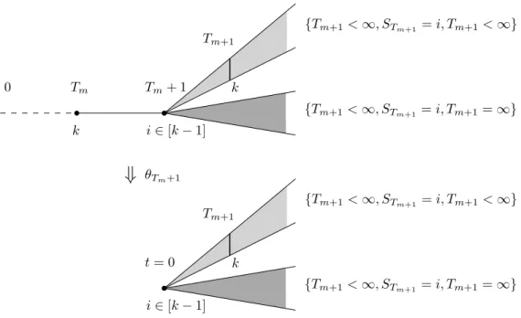
k Tm+ 1 i∈ [k − 1] {Tm+1<∞, STm+1= i, Tm+1=∞} {Tm+1<∞, STm+1 = i, Tm+1<∞} Tm+1 Tm t = 0 k k θTm+1
⇓
t = 0 i∈ [k − 1] {Tm+1<∞, STm+1= i, Tm+1=∞} {Tm+1<∞, STm+1 = i, Tm+1<∞} Tm+1 kFigure 1: The upper figure : The event tST
m`1“ i, Tm ă 8u consists of the plays that at time Tm visit state k for the mth time without ever visiting the states ą k before,
and at time Tm` 1 they visit state i, where i ă k. These plays are partitioned into two
sets. The set tTm`1 ă 8, STm`1 “ i, Tm ă 8u of plays that will visit k for the pm ` 1qth time and the set tTm`1 “ 8, STm`1 “ i, Tm ă 8u of the plays for which the mth visit in
k was the last one. The lower figure : The shift mapping θTm`1 “forgets” all the history
prior to the time Tm` 1.
Eσ‹,τ
k pϕ rk´1s
pr1,...,rk´1,η,rk`1,...,rnq˝ θTm`1| STm`1 “ i, Tmă 8q ě ξi´ δ, for all i ă k, (26) where θTm`1 is the shift mapping that deletes all history prior to the time Tm` 1.
Using the fact that for all events A and B and each integrable mapping f we have Epf | A, Bq ¨ P pAq “ Epf ¨ 1tAu| Bq we can rewrite (26) in the following form
Eσ‹,τ
k pϕ rk´1s
pr1,...,rk´1,η,rk`1,...,rnq˝ θTm`1¨1tSTm`1“iu| Tmă 8q ě
pξi´ δq ¨ Pσk‹,τpSTm`1 “ i | Tmă 8q, for i ă k. (27)
We shall prove that for i ă k, Eσ‹,τ k pϕ rk´1s pr1,...,rk´1,η,rk`1,...,rnq˝ θTm`1¨1tSTm`1“iu| Tmă 8q “ η¨Pσ‹,τ k pTm`1 ă 8, STm`1 “ i | Tm ă 8q`E σ‹,τ k pϕ rks r ¨1tTm`1“8u¨1tSTm`1“iu| Tmă 8q. (28)
Indeed the left-hand side of (28) is the sum of Eσ‹,τ k pϕ rk´1s pr1,...,rk´1,η,rk`1,...,rnq˝ θTm`1¨1tSTm`1“iu¨1tTm`1“8u| Tm ă 8q (29) and Eσ‹,τ k pϕ rk´1s pr1,...,rk´1,η,rk`1,...,rnq˝ θTm`1¨1tSTm`1“iu¨1tTm`1ă8u| Tmă 8q. (30) Consider first (30). For plays h belonging to the event tTm`1 ă 8, STm`1 “ iu, i ă k,
the shift θTm`1 removes all prefix history up to the time Tm` 1, see Figure 1. Since Tm`1ă 8 in the remaining suffix play θTm`1phq all visited states up to the next visit to
k are ă k. But for the plays that visit k at some moment and for which all states prior to this first visit to k are ă k the payoff ϕrk´1spr
1,...,rk´1,η,rk`1,...,rnq is constant and equal to
the reward η associated with k. Thus (30) is equal to η ¨ Pσ‹,τ
k pTm`1 ă 8, STm`1 “ i | Tmă 8q.
Let us examine now (29). The plays h belonging to the event tSTm`1 “ i, Tm`1 “ 8, Tm ă 8u have the following properties:
• at time Tm they visit k and all states visited prior to Tm are ď k,
• at time Tm` 1, just after the mth visit to k, they visit the state i,
• since Tm`1 “ 8 the suffix play θTm`1phq does not contain any occurrence of k (k is never visited for the pm ` 1qth time).
These properties assure that for such plays ϕrksr phq “ ϕrksr pθTm`1phqq. However, θTm`1phq has no occurrence of k, which implies for the resulting payoff it is irrelevant if k is stopping or not and what is the reward of k. Thus ϕrksr pθTm`1phqq “ ϕ
rk´1s
pr1,...,rk´1,η,rk`1,...,rnqpθTm`1phqq. This terminates the proof that (29) is equal to
Eσ‹,τ
k pϕ rks
r ¨1tTm`1“8u¨1tSTm`1“iu| Tmă 8q. This concludes also the proof of (28).
From (27) and (28) we obtain η¨Pσ‹,τ k pTm`1 ă 8, STm`1“ i | Tm ă 8q`E σ‹,τ k pϕ rks r ¨1tTm`1“8u¨1tSTm`1“iu| Tm ă 8q ě pξi´ δq ¨ Pσk‹,τpSTm`1 “ i | Tmă 8q. Summing both sides of this inequality for i ă k and rearranging the terms we obtain
ÿ iăk ξi¨ Pσk‹,τpSTm`1“ i | Tm ă 8q ď η ¨ P σ‹,τ k pTm`1 ă 8, STm`1ă k | Tmă 8q ` Eσk‹,τpϕrksr ¨1tTm`1“8u¨1tSTm`1ăku | Tm ă 8q ` δ ¨ Pσ‹,τ k pSTm`1ă k | Tmă 8q ď η ¨ Pσk‹,τpTm`1 ă 8, STm`1ă k | Tmă 8q ` Eσk‹,τpϕrksr ¨1tTm`1“8u¨1tSTm`1ăku | Tm ă 8q ` δ.
The last inequality, (24) and (25) yield η‹ ď η ¨ P σ‹,τ k pTm`1 ă 8, STm`1 ă k | Tm ă 8q `Eσk‹,τpϕrksr ¨1tTm`1“8u¨1tSTm`1ăku| Tm ă 8q `δ `η ¨ Pσk‹,τpSTm`1“ k | Tmă 8q `Eσ‹,τ k pϕ rks r ¨1tSTm`1ąku | Tm ă 8q. (31) Notice that Pσ‹,τ k pTm`1 ă 8, STm`1 ă k | Tm ă 8q ` Pkσ‹,τpSTm`1“ k | Tmă 8q “ Pσk‹,τpTm`1 ă 8 | Tm ă 8q (32)
which allows to regroup the first and the fourth summand of right-hand side of (31). Indeed, tTm`1 ă 8, Tmă 8u is the union of three disjoint events, depending on whether
the state visited at the next time moment Tm` 1 is ă k, “ k, or ą k. But for the second
of these events we have tTm`1 ă 8, Tm ă 8, STrksm`1“ ku “ tTmă 8, STrksm`1“ ku since
STrksm`1“ k implies that Tm`1 “ Tm` 1 ă 8.
And finally the third event tTm`1 ă 8, Tm ă 8, STrksm`1ą ku is empty since STrksm`1ą
k means that at time Tm`1 the game hits a stopping state thus the stopping state process
will never return to k, therefore Tm`1 “ 8. This terminates the proof of (32).
We can regroup also the second and the last summands of (31) since Pσ‹,τ
k pTm`1 “ 8, STm`1 ă k | Tm ă 8q ` Pkσ‹,τpSTm`1ą k | Tmă 8q
“ Pσ‹,τ
k pTm`1 “ 8 | Tmă 8q
We obtain this again by presenting the event tTm`1 “ 8, Tm ă 8u as the union of
three disjoint events depending on the value of STm`1. However, STm`1 “ k contradicts
Tm`1“ 8 and STm`1 ą k implies Tm`1“ 8.
Using these observations we deduce from (31) that η‹ď η ¨ P σ‹,τ k pTm`1ă 8 | Tm ă 8q ` Eσk‹,τpϕrksr ¨1tTm`1“8u| Tm ă 8q ` δ. (33)
Since ϕrksr ď 1, from (33) we obtain that
η ¨ Pσ‹,τ
k pTm`1 ă 8 | Tmă 8q ` Pkσ‹,τpTm`1 “ 8 | Tmă 8q ě η‹´ δ.
But Pσ‹,τ
k pTm`1 “ 8 | Tm ă 8q ` Pσk‹,τpTm`1 ă 8 | Tm ă 8q “ 1 thus the last
inequality yields Pσ‹,τ k pTm`1 ă 8 | Tm ă 8q ď 1 ` δ ´ η‹ 1 ´ η ă 1 ` pη‹´ ηq ´ η‹ 1 ´ η “ 1.
Therefore Pσ‹,τ k p@m, Tmă 8q “ limmÑ8P σ‹,τ k p@i ď m, Tiă 8q “ lim mÑ8P σ‹,τ k pT0 ă 8q ¨ m´1 ź q“0 Pσ‹,τ k pTq`1ă 8 | Tq ă 8q ď lim mÑ8 ˆ 1 ´ η‹` δ 1 ´ η ˙m´1 “ 0, (34)
i.e. if player Max uses the strategy σ‹ then with probability 1 the state k is visited
only finitely many times.
Multiplying both sides of (33) by Pσ‹,τ
k pTm ă 8q, taking into account that 0 ă δ ă
η‹´ η and rearranging we get
Eσ‹,τ k pϕ rks r ¨1tTm`1“8u¨1tTmă8uq ą η ¨ P σ‹,τ k pTmă 8q ´ η ¨ Pσk‹,τpTm`1 ă 8, Tm ă 8q “ η ¨ Pσ‹,τ k pTm`1 “ 8, Tm ă 8q. (35)
Since the events tTm`1 “ 8, Tm ă 8umě0 and t@m, Tm ă 8u form a partition of
the sets of plays but the last event has probability 0, summing up both sides of (35) for all m ě 1 we obtain Eσ‹,τ k pϕ rks r q ą η ą wk´ ε 2
which terminates the proof of the right-hand side inequality in (??).
6.2 ε{2-optimal strategy τ‹ for player Min when wk ě rk and k is the
starting state.
We assume that wk ě rk and ε ą 0. The aim of this section is to construct a strategy
τ‹ for player Min such that
Eσ,τ‹
k pϕ rks
r q ď wk` ε{2 (36)
for each strategy σ of Max.
The strategy τ‹ of player Min is constructed in the following way.
(i) If the current state is k then player Min selects actions with probability given by his optimal strategy in the one-day game Mkpw1, . . . , wk´1, wk, rk`1, . . . , rnq.
Thus the strategy of player Min at k is “locally memoryless”, the probability used to select actions to execute at k does not depend on the previous history.
(ii) During all stages j such that Tm ă j ă Tm`1 (between the mth and pm ` 1qth
visit to state k) player Min plays using his εm :“ ε{2m`1-optimal strategy in the
ϕrk´1spr
1,...,rk´1,wk,rk`1,...,rnq-game
6. In general the strategy played by Min between two
visits to state k is not memoryless because εm changes at each visit to k.
When player Min applies this strategy during all stages j, Tm ă j ă Tm`1, in
the ϕrksr -game then we assume tacitly that starting from stage Tm` 1 player Min
“forgets” all history preceding this stage and he plays this strategy as if the game started afresh at stage Tm` 1.
From the optimality of τ‹ in the one-day game Mkpw1, . . . , wk´1, wk, rk`1, . . . , rnq
we obtain ÿ jăk wj¨ Pσ,τk ‹pSTrksm`1“ j|Tm ă 8q ` wk¨ Pσ,τk ‹pS rks Tm`1“ k|Tmă 8q (37) `ÿ jąk rj¨ Pσ,τk ‹pSTrksm`1“ j|Tm ă 8q ď wk.
Indeed, at the time Tmthe current visited state is k and player Min selects actions
ac-cording to his optimal strategy in the one-day game Mkpw1, . . . , wk´1, wk, rk`1, . . . , rnq
and, by (16), the left-hand side of (37) gives the payoff in this one-day game while the right-hand side is the value of this game. Since he plays optimally the payoff cannot be greater than the value.
Let us consider the event
tTm ă 8, STm`1“ iu, where i ă k. (38)
This event, presented on the upper side of Figure 1, consists of plays h satisfying the following conditions:
(i) h visits k at least m times and prior to the m-th visit to k (which takes place at time Tm) the stopping states tk ` 1, . . . , nu were not visited, i.e. St P rks for all
t ă Tm,
(ii) at time Tm the game moves from k to i, i.e. STm`1“ i.
The definition of τ‹says that starting from time Tm`1, if the current state STm`1is ă
k and until the next visit to state k, player Min plays according to ε{2m`1-optimal
strat-egy in the ϕrk´1spr
1,...,rk´1,wk,rk`1,...,rnq-game. By (15), the value of the ϕ
rk´1s
pr1,...,rk´1,wk,rk`1,...,rnq -game starting at state i P rk ´ 1s is wi.
Thus if we consider the game that, in some sense, restarts afresh at state i at time Tm` 1 and we apply to such residual game the payoff ϕrk´1spr1,...,rk´1,wk,rk`1,...,rnq and we
assume that player Min plays τ‹ then the expected payoff will not be greater than
wi` ε{2m`1, i.e. Eσ,τ‹ k pϕ rk´1s pr1,...,rk´1,wk,rk`1,...,rnq˝ θTm`1 | STm`1“ i, Tmă 8q ď wi` ε{2 m`1. (39)
where f ˝ g denotes the composition of mapping f and g.
Now let us note that (37) closely resembles (24) while (39) resembles (26). What is different but symmetric is that the first two formulas concern strategies pσ‹, τ q and the
last two pσ, τ‹q. Moreover, the inequalities are reversed. The following table resumes the
correspondence between constants appearing in the formulas: Eq. (24), (26) Eq. (37), (39)
η wk
η‹ wk
ξi wi
δ ´εm
Thus exactly in the same way as we deduced (33) from (26) and (24) we can deduce from (37) and (39) the following formula analogous to (33) (just reverse the inequality and replace the constants as indicated above):
wk¨ Pσ,τk ‹pTm`1 ă 8 | Tmă 8q
`Eσ,τk ‹pϕrksr ¨1tTm`1“8u| Tm ă 8q ´εmď wk.
Rearranging the terms and multiplying by Pσ,τ‹
k pTm ă 8q we obtain from this inequality
that Eσ,τ‹ k pϕ rks r ¨1tTm`1“8u¨1tTmă8uq ď wk¨ P σ,τ‹ k pTm`1“ 8, Tmă 8q ` ε 2m`1 ¨ P σ,τ‹ k pTm ă 8q ď wk¨ Pσ,τk ‹pTm`1“ 8, Tmă 8q ` ε 2m`1.
The events tTm`1 “ 8, Tm ă 8u are pairwise disjoint and their union is equal to
tDm, Tm“ 8u thus summing over m ě 1 both sides of the inequality we obtain
Eσ,τ‹
k pϕ rks
r ¨1tDm,Tm“8uq ď wk¨ Pσ,τk ‹pDm, Tm“ 8q ` ε{2.
On the other hand, for all plays in t@m, Tm ă 8u the state k is visited infinitely often
thus ϕrksr is equal to rk. Thus Eσ,τ‹ k pϕ rks r q “ E σ,τ‹ k pϕ rks r ¨1tDm,Tm“8uq ` E σ,τ‹ k pϕ rks r ¨1t@m,Tm“8uq “ Eσ,τ‹ k pϕ rks r ¨1tDm,Tm“8uq ` rk¨ Pσ,τk ‹p@m, Tmă 8q ď wk¨ Pσ,τk ‹pDm, Tm“ 8q ` rk¨ Pσ,τk ‹p@m, Tmă 8q ` ε{2 ď wk` ε{2.
6.3 ε{2-optimal strategies for the other cases when the starting state is k
In Sections 6.1and6.2we have constructed ε{2-optimal strategies for player Max when wką rk and for player Min when wkě rk under the condition that Fixk´1pf qprq is the
value vector of the ϕrk´1sr -game.
But passing to the dual game, the last condition implies that Fixk´1
pf qprq is the value vector in the dual stopping game with payoff ϕrk´1sr .
Therefore, proceeding exactly as in Section 6.1, we can construct a strategy τ‹ for
player Max in the dual game with payoff ϕrksr such that
Eτk‹,σpϕrksr q ěwk´ ε{2 (40)
for all strategies σ of player Min if
wką rk. (41)
By duality of games and fixed points, Ekτ‹,σpϕrksr q “ 1 ´ Ekσ,τ‹pϕrksr q, wk“ 1 ´ wk and
rk“ 1 ´ rk. Thus (40) is equivalent to Eσ,τ
‹
k pϕ rks
r q ď wk` ε{2 and (41) is equivalent to
wkă rk, i.e. we get a ε{2-optimal strategy of player Min in the ϕrksr -game if wkă rk.
In the similar way, applying the construction of Section6.2to the dual game and com-ing back to the original game we get a strategy σ‹for player Max such that Eσ‹,τ
k pϕ rks r q ě
wk´ ε{2 if wk ď rk.
6.4 ε-optimal strategies for the ϕrksr -game starting at states ă k.
It remains to prove that
Fixkipf qprq :“ Fik´1pwk; rq
is the value of the ϕrksr -game starting in the state i ă k. To this end we must construct
strategies σ7 and τ7 for player Max and Min, respectively, such that
Eσ,τ7 i pϕ rks r q ď Fixkipf qprq ` ε and E σ7,τ i pϕ rks r q ě Fixkipf qprq ´ ε (42)
for all strategies σ, τ . We define only the strategy τ7 for player Min and prove the first
equation of (42). The definition of σ7 and the proof of the right-hand side of (42) are
symmetrical and are left to the reader.
Recall that T1 was defined as the (random) time of the first visit of the stopped
state process Strks to the state k, cf. (17). Let τ‹ be the strategy of player Min defined
at page 26 that satisfies (36), i.e τ‹ is an ε{2-optimal for player Min in the ϕ rks r -game
starting at the state k.
By the induction hypothesis, there exists an ε{2-optimal strategy α for player Min in the ϕrk´1spr
1,...,rk´1,wk,rk`1,...,rnq-game.
τ7pS1, A1, B1, ¨ ¨ ¨ , Smq “
#
αpS1, A1, B1, ¨ ¨ ¨ , Smq if T1 ą m,
τ‹pST1, AT1, BT1, ¨ ¨ ¨ , Smq if T1 ď m.
Intuitively, τ7 is the strategy such that player Min plays according to α until the first
visit to k and starting from the moment of the first visit to k he switches to τ‹. Moreover,
when he switches to τ‹ then he “forgets” all history prior to the moment T1 and behaves
as if the game have started afresh at k.
First we want to show that, for each strategy σ of player Max and for each state i ă k,
Eσ,τ7
i pϕrksr | T1 ă 8q “ E σ,τ7
i pϕrksr ˝ θT1 | T1 ă 8q ď wk` ε{2 where θT1 is the shift operation, cf. Definition12, and wk “ Fix
k
kpf qprq is the value of
k.
To justify the first equality let us notice that the plays with T1ă 8 do not visit the
stopping states, i.e. the states ą k, prior to T1. Therefore the payoff ϕrksr for such plays
is not modified if we shift them by T1.
The second inequality follows from the definition of τ7. When the game hits state k
at time T1player Min switches to strategy τ‹and forgets the history prior to T1. Since τ‹
is ε{2-optimal for player Min in the ϕrksr -game for plays starting at k, using this strategy
limits the payoff to at most wk` ε{2.
Now we examine the expected payoff for plays with T1 “ 8. Such plays never visit
k, therefore it is irrelevant for them if k is stopping or not like it is irrelevant what is the reward associated with k. Moreover, for such plays player Min plays according to strategy τ‹. For these reasons we have
Eσ,τ7 i pϕrksr | T1“ 8q “ Eσ,τi ‹pϕ rk´1s pr1,...,rk´1,wk,rk`1,...,rnq| T1 “ 8q. (43) From (43) we obtain Eσ,τ7 i pϕrksr q “ E σ,τ7 i pϕrksr | T1ă 8q ¨ P σ,τ7 i pT1 ă 8q ` Eσ,τi 7pϕrksr | T1“ 8q ¨ P σ,τ7 i pT1 “ 8q ď pwk` ε{2q ¨ P σ,τ7 i pT1 ă 8q ` Eσ,τi ‹pϕrk´1spr 1,...,rk´1,wk,rk`1,...,rnq| T1“ 8q ¨ P σ,τ7 i pT1 “ 8q. (44)
Since τ‹ is ε{2-optimal for player Min in the ϕ rk´1s pr1,...,rk´1,wk,rk`1,...,rnq-game we have Fik´1pwk; rq ` ε{2 ě Eσ,τi ‹pϕ rk´1s pr1,...,rk´1,wk,rk`1,...,rnqq “ Eσ,τi ‹pϕrk´1spr 1,...,rk´1,wk,rk`1,...,rnq| T1 ă 8q ¨ P σ,τ‹ i pT1ă 8q ` Eσ,τi ‹pϕrk´1spr 1,...,rk´1,wk,rk`1,...,rnq| T1 “ 8q ¨ P σ,τ‹ i pT1“ 8q.
![Figure 2: Game SKIRMISH [3].](https://thumb-eu.123doks.com/thumbv2/123doknet/14320414.496967/33.892.239.576.808.965/figure-game-skirmish.webp)
