HAL Id: hal-01447351
https://hal.archives-ouvertes.fr/hal-01447351
Submitted on 26 Jan 2017
HAL is a multi-disciplinary open access
archive for the deposit and dissemination of
sci-entific research documents, whether they are
pub-lished or not. The documents may come from
teaching and research institutions in France or
abroad, or from public or private research centers.
L’archive ouverte pluridisciplinaire HAL, est
destinée au dépôt et à la diffusion de documents
scientifiques de niveau recherche, publiés ou non,
émanant des établissements d’enseignement et de
recherche français ou étrangers, des laboratoires
publics ou privés.
Bayesian joint estimation of the multifractality
parameter of image patches using gamma Markov
Random Field priors
Sébastien Combrexelle, Herwig Wendt, Yoann Altmann, Jean-Yves Tourneret,
Stephen Mclaughlin, Patrice Abry
To cite this version:
Sébastien Combrexelle, Herwig Wendt, Yoann Altmann, Jean-Yves Tourneret, Stephen Mclaughlin, et
al.. Bayesian joint estimation of the multifractality parameter of image patches using gamma Markov
Random Field priors. IEEE International Conference on Image Processing (ICIP 2016), Sep 2016,
Phoenix, United States. pp. 4468-4472. �hal-01447351�
O
pen
A
rchive
T
OULOUSE
A
rchive
O
uverte (
OATAO
)
OATAO is an open access repository that collects the work of Toulouse researchers and
makes it freely available over the web where possible.
This is an author-deposited version published in :
http://oatao.univ-toulouse.fr/
Eprints ID : 17200
The contribution was presented at ICIP 2016 :
http://2016.ieeeicip.org/
To cite this version :
Combrexelle, Sébastien and Wendt, Herwig and Altmann,
Yoann and Tourneret, Jean-Yves and Mclaughlin, Stephen and Abry, Patrice
Bayesian joint estimation of the multifractality parameter of image patches using
gamma Markov Random Field priors. (2016) In: IEEE International Conference
on Image Processing (ICIP 2016), 25 September 2016 - 28 September 2016
(Phoenix, United States).
Any correspondence concerning this service should be sent to the repository
administrator:
staff-oatao@listes-diff.inp-toulouse.fr
BAYESIAN JOINT ESTIMATION OF THE MULTIFRACTALITY PARAMETER OF IMAGE
PATCHES USING GAMMA MARKOV RANDOM FIELD PRIORS
S. Combrexelle
1, H. Wendt
1, Y. Altmann
2, J.-Y. Tourneret
1, S. McLaughlin
2, P. Abry
31IRIT - ENSEEIHT, CNRS, Univ. of Toulouse, F-31062 Toulouse, France, firstname.lastname@enseeiht.fr 2School of Engineering and Physical Sciences, Heriot-Watt Univ., Edinburgh, UK, initial.lastname@hw.ac.uk 3CNRS, Physics Dept., Ecole Normale Sup´erieure de Lyon, F-69364 Lyon, France, patrice.abry@ens-lyon.fr
ABSTRACT
Texture analysis can be embedded in the mathematical frame-work of multifractal (MF) analysis, enabling the study of the fluctu-ations in regularity of image intensity and providing practical tools for their assessment, wavelet leaders. A statistical model for lead-ers was proposed permitting Bayesian estimation of MF parametlead-ers for images yielding improved estimation quality over linear regres-sion based estimation. This present work proposes an extenregres-sion of this Bayesian model for patch-wise MF analysis of images. Classi-cal MF analysis assumes space homogeneity of the MF properties whereas here we assume MF properties may change between texture elements and we do not know where the changes are located. This paper proposes a joint Bayesian model for patches formulated using spatially smoothing gamma Markov Random Field priors to coun-terbalance the increased statistical variability of estimates caused by small patch sizes. Numerical simulations based on synthetic multi-fractal images demonstrate that the proposed algorithm outperforms previous formulations and standard estimators.
Index Terms— Multifractal Analysis, Wavelet Leaders, Bayesian Estimation, Texture Analysis, Gamma Markov Random Field
1. INTRODUCTION
Context. Texture analysis is an important field in image process-ing conducted usprocess-ing various paradigms [1]. Among them, the math-ematical framework of multifractal analysis has recently proven to be particularly relevant, cf., e.g., [2, 3] and references therein. Mul-tifractal analysis describes the image texture in terms of the spatial fluctuations of the degree of smoothness of the image intensity at each point. More precisely, the texture of an image X is quantified by means of the multifractal spectrum D(h), which is defined as the Hausdorff dimension of the sets of points that possess the same pointwise H¨older regularityh, cf., e.g., [4–7].
Multifractal models are specific instances of scale invariant models and can be practically assessed by studying, over a range of scales 2j, the power law behaviors of the sample moments of suitably designed multiresolution quantities TX(j, k) of X (i.e., quantities that depend jointly on scale2jand spatial position k)
S(q, j), n1 j
X k
|TX(j, k)|q≃ (2j)ζ(q), j1≤ j ≤ j2 (1) wherenj = card(TX(j,·)) is the number of TX(j, k) at scale j. The multiresolution quantities used in this work are the wavelet
lead-This work was supported by ANR BLANC 2011 AMATIS BS0101102. S. Combrexelle was supported by the Direction G´en´erale de l’Armement (DGA). SML acknowledges the support of EPSRC via grant EP/J015180/1.
ersl(j, k) (defined in Section 2), which can be shown to be specifi-cally appropriate for multifractal analysis purposes [2, 5].
The scaling exponentsζ(q) characterizing the power law behav-ior in (1) are intimately tied to the multifractal spectrum of the image by a Legendre transform,D(h)≤ L(h) , infq∈R[2 + qh− ζ(q)], and this link enables the practical assessment of multifractal models. Specifically, it permits discrimination between the two most impor-tant classes of models: Self-similar models [8], which translate into a strictly linear behavior ofζ(q) in the neighborhood of q = 0; Mul-tifractal multiplicative cascade (MMC) based processes [9] which yield a strictly concave functionζ(q). This difference can be quanti-fied by considering the coefficients of a polynomial development of ζ(q) at the origin, ζ(q) =Pm≥1cmqm/m! [2, 10, 11]. In particu-lar, it can be shown that the second coefficientc2, called the
multi-fractality parameter, is identically zero for self-similar processes but strictly negative for MMC [5, 11]. It therefore enables us to decide which model is better adapted to data in applications, which renders its estimation a central element in multifractal analysis. The reader is referred to, e.g., [4–7], for further details on multifractal analysis. Estimation ofc2for image patches. The multifractality param-eterc2 can be shown to be directly linked to the variance of the logarithm of the multiresolution quantities [10]
C2(j), Var [ln l(j, k)] = c02+ c2ln 2j. (2) This leads to the definition of the standard estimation procedure for c2 as a linear regression of the sample variance dVar[·] of the log-leaders with respect to scalej
ˆ c2= 1 ln 2 j2 X j=j1 wjdVar[ln l(j,·)] (3) wherewj are appropriate regression weights [2, 12, 13]. While the simplicity of (3) is attractive, the estimator is known to yield poor performance (large variance) even for moderate image size, which strongly limits its relevance for the analysis of image patches.
An attempt to improve estimation performance was described in [14], which introduced an estimator based on the generalized method of moments. However, this estimator relies on fully parametric mod-els that are too restrictive for real-world images. More recently, Bayesian estimators ofc2have been investigated for images of rel-atively small sizes [3, 15]. At the core of this approach is a generic semi-parametric model for the statistics of the log-leaders whose variance-covariance structure is controlled byc2. This model leads to a likelihood that can be efficiently evaluated with a closed-form Whittle approximation. The Bayesian inference was achieved by a Markov chain Monte Carlo (MCMC) algorithm with a Metropolis-Hastings within Gibbs (MHG) sampler. In [16], an alternative data-augmented formulation for the Bayesian model was proposed which
complies with the use of conjugate priors, hence yielding a more effi-cient algorithm. While the method significantly improves estimation performance over (3), the variance of estimates for image patches is still too large for practical applications.
Goals and contributions. The goal of this paper is to devise a Bayesian procedure for the joint estimation ofc2for image patches which further improves the estimation performance of the Bayesian estimator introduced in [16] by exploiting the spatial dependence be-tween patches through appropriate priors, while inheriting the favor-able computational cost of [16]. Starting from the statistical model for a single image introduced in [3, 15, 16] (recalled in Section 2), the proposed procedure relies on the following original key ingredi-ents (detailed in Section 3). First, the joint likelihood of all image patches is expressed as the product of the augmented likelihood of each individual patch given by [16]. Then, a hidden gamma Markov random field (GMRF) [17] with four-fold spatial neighborhood is assigned as a joint prior for the multifractality parameters of the im-age patches. It relies on the use of a set of auxiliary variables that model positive dependence between the parameters of neighboring image patches. The GMRF prior and data augmentation scheme are designed in such a way that the conditional distributions of the re-sulting joint posterior can be sampled directly (and thus efficiently), without the need of Metropolis-Hastings steps. The computation of the Bayesian estimator associated with the proposed model is per-formed by means of an MCMC algorithm, which samples an appriate target distribution resulting from the data augmentation pro-cedure to then approximate Bayesian estimators of the variables of interest.
The performance of the joint estimation procedure of parametersc2 associated with image patches is studied in Section 4 by numeri-cal simulations conducted with synthetic multifractal images. These images have prescribed piece-wise homogeneous multifractal prop-erties yielding a controlled ground truth. The proposed method sig-nificantly outperforms the linear regression (3), reducing root mean squared error (RMSE) values by one order of magnitude, as well as the Bayesian estimators in [3, 15, 16]. It enables, for the first time, the reliable assessment of small local changes inc2between image patches.
2. STATISTICAL MODEL FOR LOG-LEADERS 2.1. Time-domain statistical model
Wavelet leaders. 2D wavelets are commonly defined as tensorial products of the scaling functionφ(x) and mother wavelet ψ(x) of a 1D multiresolution analysis,ψ(0)(x) = φ(x1)φ(x2), ψ(1)(x) = ψ(x1)φ(x2), ψ(2)(x) = φ(x1)ψ(x2), ψ(3)(x) = ψ(x1)ψ(x2) [18, 19]. Whenψ is suitably chosen, the dilated and translated templates denotedψ(m)j,k (x) = 2−j/2ψ(m)(2−jx− k) ψ(m), wherea = 2j and x = 2jk, k = (k
1, k2), form a basis of L2(R2). The L1 normalized discrete wavelet transform coefficients of an image X are defined asd(m)X (j, k) ="X, 2−j/2ψ(m)
j,k #, m = 0, . . . , 3 [18]. Letλj,kdenote the dyadic cube of side length2jcentred at k2j and3λj,k=!n1,n2={−1,0,1}λj,k1+n1,k2+n2the union with its eight
neighbors. The wavelet leaders are defined as the supremum of the wavelet coefficients within3λj,kover all finer scales [2, 5], i.e.,
l(j, k), sup m∈(1,2,3),λ′⊂3λ
j,k
|d(m)X (λ′)|. (4) Statistical model. We denote by ℓj the vector of all log-leaders ℓ(j,·) , ln l(j, ·) at scale j after mean subtraction (the mean does
not convey any information onc2). It has recently been shown that for MMC based processes, the statistics of ℓj can be well ap-proximated by a multivariate Gaussian distribution whose covari-anceCj(k, ∆k), Cov[ℓ(j, k), ℓ(j, k + ∆k)] is modeled by a ra-dial symmetric function parametrized only by θ= (c2, c02)
Cj(k, ∆k)≈ ̺j(||∆k||; θ) , " ̺0 j(||∆k||; θ) ||∆k|| ≤ 3 ̺1j(||∆k||; θ) 3 < ||∆k|| (5)
where|| · || is the Euclidian norm, ̺0
j(r; θ), ajln(1 + r) + c02+ c2ln 2j with aj , (̺1j(3; θ)− c02− c2ln 2j)/ln 4, ̺1j(r; θ) , c2ln(4r/√nj)I[0,√nj/4](r), IAis the indicator function of the set
A, cf., [3]. Under these assumptions, the likelihood of ℓjis given by p(ℓj|θ) ∝ |Σj,θ|− 1 2exp # −1 2ℓ T jΣ−1j,θℓj $ (6) where the covariance matrix Σj,θis defined by̺j(||∆k||; θ), | · | is denoting the determinant andT the transpose operator.
Whittle approximation. The evaluation of the above likelihood is problematic even for small images since it requires computing the matrix inverse Σ−1j,θ. Thus, it has been proposed in [3, 15] to approx-imate (6) with the asymptotic Whittle likelihood [20–24]
pW(ℓj|θ)=exp % −X m∈Jj ln φj(m; θ) + y∗j(m)yj(m) φj(m; θ) & . (7)
Here, m are the indices of the frequencies ωm = 2πm/√nj of the discrete Fourier transform for one Fourier half-plane1Jj, yj , F(ℓj) where the operatorF(·) computes and vectorizes the discrete Fourier transform coefficients contained inJjand∗stands for com-plex conjugation. The functionφj(m; θ) corresponds to the dis-cretized parametric spectral density associated with the model (5) and has a closed-form parametric expression given byφj(m; θ) = c2fj(m)+c02gj(m), where fjandgjdo not depend on θ and can be precomputed and stored in two vectors denoted as fj,(fj(m))m∈J
j
and gj,(gj(m))m∈J
j, see [15] for details. Furthermore,
indepen-dence is assumed between different scalesj, which leads to the fol-lowing Whittle likelihood for all log-leaders ℓ, [ℓT
j1, . . . , ℓ T j2] T pW(ℓ|θ) = j2 ' j=j1 pW(ℓj|θ). (8)
2.2. Data augmented statistical model in the Fourier domain The parameters θ are encoded implicitly in Σ−1j,θ, and their condi-tional distributions are thus not standard. Sampling the posterior distribution with an MCMC method would thus require accept/reject procedures, such as MHG moves [3]. To obtain a more efficient al-gorithm, (8) can be interpreted as a statistical model for the Fourier coefficients yj[16]. More precisely, (8) can be rewritten as
pW(ℓ|θ) =|Γθ|−1exp # −yHΓ−1θ y $ , (9) y, [yT j1, ..., y T j2] T, yj =F(ℓj)
whereHis the conjugate transpose operator and theNY× NY diag-onal covariance matrix Γθ, withNY , card(y), is given by Γθ , 1Note that due to properties of Fourier transform of real functions, only
c2F + c02G with F , diag (f), G , diag (g), f , [fjT1, ..., f T j2] T and g , [gT j1, ..., g T j2] T. Assuming that Γ θis positive definite, (9) amounts to modeling the Fourier coefficients y by a random vector with a centered circular-symmetric complex Gaussian distribution CN (0, Γθ) [25], hence to the use of the likelihood
p(y|θ) = |Γθ|−1exp #
−yHΓ−1θ y $
. (10) Reparametrization. The matrix Γθis positive definite as long as the parameters θ= (c2, c02) belong to the admissible set
A = {θ ∈ R−⋆×R+⋆|c2f(k)+c02g(k) > 0, k = 1, . . . , NY}. (11) It can be shown that∀k, c0
2g(k) > 0 (while∃k|f(k) < 0) [15] and hence that (11) can be transformed into independent positiv-ity constraints after reparametrization by the mapping θ 2→ v , (−c2, c02/γ + c2), where γ = supkf(k)/g(k) [16]. This map de-fines a one-to-one transformation from θ∈ A to v ∈ R+2
⋆ and (10) can be expressed with v as
p(y|v) ∝|Γv|−1exp # −yHΓ−1v y $ (12) Γv= v1F˜+ v2G,˜ F˜=−F + Gγ, G˜= Gγ. where the diagonal matrices ˜F , ˜G and Γv, for v ∈ R+2⋆ , are by construction positive definite.
Data augmentation. The likelihood (12) is finally extended using the model y|µ, v2∼ CN (µ, v2G), µ˜ |v1∼ CN (0, v1F˜), where µ is anNY × 1 vector of additional latent variables [16]. This model is associated with the extended likelihood
p(y, µ|v) ∝ v2−NY exp # −v1 2(y− µ) H˜ G−1(y− µ)$ × v1−NYexp # −v1 1µ H˜ F−1µ $ (13) from which (12) can be recovered by marginalization with respect to µ. One easily verifies that (13) leads to standard conditional distri-butions when inverse-gamma (IG) priors are used for vi∈ R+⋆.
3. BAYESIAN ESTIMATION FOR IMAGE PATCHES Based on the likelihood (13) for one single image (or patch), we now formulate our joint Bayesian model for image patches.
3.1. Likelihood
Denote as{Xk} a partition of the image X into non-overlapping patches Xk of sizeN × N, and as yk, µk and vkthe Fourier coefficients, latent variables and parameter vector associated with patch Xk. Let furthermore denote Y , {yk}, M , {µk}, and V , {V1, V2} with Vi, {vi,k}, i = 1, 2. With the assumptions of Section 2, the joint likelihood of Y can be written
p(Y , M|V ) ∝' k
p(yk, µk|vk). (14)
3.2. Gamma Markov random field prior
Inverse-gamma distributions IG(αi,k, βi,k) are conjugate priors for the parameters vi,k in (14), where i = 1, 2. We propose here to specify (αi,k, βi,k) such that the resulting prior for Vi is a hidden GMRF [17], which relies on the use of a set of
positive auxiliary variables Z = {Z1, Z2}, Zi = {zi,k}, to induce positive dependence between the neighbooring elements of Vi [17] and hence spatial regularization. More precisely, eachvi,k is connected to the four auxiliary variableszi,k′ > 0,
k′∈ Vv(k), {(k1, k2), (k1+1, k2), (k1, k2+1), (k1+1, k2+1)} (and thus, eachzi,k to vi,k′, k′ ∈ Vz(k) = {(k1 − 1, k2 −
1), (k1, k2− 1), (k1− 1, k2), (k1, k2)}), via edges weighted by ai, which act as a regularization parameters controlling the amount of spatial smoothness. This GMRF prior for(Vi,Zi) can be shown to be associated with the density [17]
p(Vi, Zi|ai) = C(ai)−1 '
ke
−(4ai+1) log vi,ke(4ai−1) log zi,k
× e− ai vi,k P k′ ∈Vv (k)zi,k′ (15) whereC(ai) is an (intractable) normalization constant.
Posterior. Assuming prior independence between(V1, Z1) and (V2, M , Z2), Bayes’ theorem yields the joint posterior distribution associated with the proposed model
p(V , Z, M|Y , a1, a2) ∝ p(Y |V2, M ) p(M|V1)
× p(V1, Z1|a1) p(V2, Z2|a2) (16) whereai,i = 1, 2, are fixed hyperparameters.
3.3. Bayesian estimators
Since we are interested in the parameters Vi only, we consider the marginal posterior mean estimator for Vi, denoted MMSE (minimum mean square error estimator) and defined as VMMSEi , E[Vi|Y , ai], where the expectation is taken with respect to the marginal posterior densityp(Vi|Y , ai). Note that the direct compu-tation of VMMSE
i is not tractable as it requires integrating the full pos-terior (16) over all other unknown variables. By considering a Gibbs sampler (GS) drawing samples ({V(k)i }, M(k),{Zi(k)})Nk=1mc asymptotically distributed according to (16), we can however ap-proximate VMMSEi using the samples V
(k) i [26] as VMMSEi ≈ (Nmc− Nbi)−1 XNmc k=Nbi V(k)i (17) whereNbiis the length of the burn-in period.
3.4. Gibbs sampler
The GS consists of successively generating samples from the con-ditional distributions associated with the target distribution, here the posterior [26]. The conditionals for (16) can be easily calculated
µk|Y ,V ∼CN # v1,kF Γ˜ −1vkyk, # (v1,kF˜)−1+(v2,kG)˜ −1 $−1$ (18a) v1,k|M,Z1∼IG ( NY+α1,k,||µk||F˜−1+β1,k ) (18b) v2,k|Y ,M,Z2∼IG ( NY+α2,k,||yk−µk||G˜−1+β2,k ) (18c) zi,k|Vi∼G(˜αi,k, ˜βi,k) (18d) where||x||Π,xHΠx, αi,k= ˜αi,k= 4ai,βi,k= aiPk′∈V
v(k)zi,k′
and ˜βi,k = (aiPk′∈V z(k)v
−1
i,k′)−1. Note that all conditionals
(18a–18d) are standard laws that can be sampled efficiently, without Metropolis-Hastings acceptance-reject steps.
Finally, note that it is easy to show that assuming independence between parametersvi,k, that have inverse-gamma priorsIG(ci, di) instead of (15), leads to a Bayesian model that can be sampled using GS steps defined in (18a–18c) with parametersαi,k= ciandβi,k= di. This model is equivalent to the one studied in [16].
Fig. 1. Mask of piecewise constant values ofc2∈ {−0.02, −0.04} (middle); one realization of MRW with the values ofc2displayed in the middle figure (right).
4. NUMERICAL EXPERIMENTS
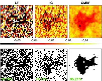
The proposed Bayesian estimator for the multifractality parameters associated with image patches (with spatial GMRF prior, denoted GMRF) was applied to independent realizations of 2D multifrac-tal random walks (MRWs) of size2048× 2048, with two distinct zones of homogeneous multifractality. MRWs are MMC processes that have multifractal properties similar to those of Mandelbrot’s log-normal cascades, with scaling exponentsζ(q) = (H− c2)q + c2q2 (cf., [27] for details). A typical realization is plotted in Fig. 1 (right) together with the zones of constant multifractality parameter used here (a polygon with c2 = −0.04 and a background with c2 = −0.02). This piece-wise constant spatial evolution of c2 is cho-sen here as a limit case test for GMRF (which is actually designed for smooth evolutions). We use non-overlapping patches of size N×N = 64×64 and compare the proposed estimator with its coun-terpart withIG prior of [16] (denoted IG) and the standard linear re-gression based estimator (using (3) with weightswj as in [2, 12, 13] and denoted as LF). The regularization parameters of GMRF have been fixed toai = 10 using cross-validation (note that results have been found to be robust with respect to the precise choice ofai). Illustration for a single realization. Fig. 2 (top row) shows patch-wise estimates ofc2obtained with LF, IG and GMRF (from left to right). Clearly, LF fails to reveal the two zones with distinct val-ues of c2 in the image. The Bayesian estimator IG improves the estimation quality significantly as compared to LF and enables the visual identification of the polygon. Yet, estimates obtained with IG still display strong variability. In contrast, the proposed Bayesian estimator with GMRF prior yields excellent estimates that closely reproduce the prescribed zones with constantc2. A more quanti-tative analysis is proposed in Fig. 2 (bottom row), which shows the results of a classification of the patch-wise estimates ofc2, ob-tained by histogram thresholding using the k-means algorithm with 2 classes. Classification performance is quantified as the percentage of correctly classified pixels in the image and is stated in color in the figure. The results further confirm the above conclusions: LF yields classification performance that is not better than that of random clas-sification; IG enables approximately three quarters of the pixels to be correctly classified; GMRF yields excellent classification results and 95% correctly classified pixels.
Estimation performance. The estimation performance is as-sessed through the bias, the standard deviation (STD) and the root mean squared error (RMSE) of the different estimators computed for 100 independent realizations and defined by b = *E[ˆc2]− c2, s= ( +Var[ˆc2])
1
2 and rms=,b2+ s2, respectively. Moreover, we
compute the average of correctly classified pixels (denoted ccp)
Fig. 2. Patch-wise estimation ofc2for a single realization of MRW (top; the ground truth and data are plotted in Fig. 1); k-means clas-sification of the estimates (bottom).
for k-means classification of patch-wise estimates as described in the previous paragraph. Results are summarized in Table 1 and strengthen the above conclusions. While the Bayesian estimator IG improves STD and RMSE values by a factor of3−4 as compared to LF as reported in [16], the proposed Bayesian estimator GMRF further and significantly improves STD and RMSE values to only 1/10th of those of LF. The excellent performance of GMRF is also reflected by the classification results: GMRF yields by far the best ccp equal to94.6%. Finally, note that these performance improve-ments are achieved at only≈ 5 times the computational time of LF.
|b| s rms ccp
LF 0.0055 0.0406 0.0413 54.2 IG 0.0018 0.0123 0.0125 76.5 GMRF 0.0027 0.0032 0.0044 94.6 Table 1. Estimation performance for100 independent realizations.
5. CONCLUSIONS AND FUTURE PERSPECTIVES This work investigated a Bayesian model that enables the joint esti-mation of the multifractality parametersc2 of image patches. This relied on the use of a recently proposed data augmented Whittle likelihood for log-leaders and on a suitable GMRF joint prior for the multifractality parameters. This prior efficiently counteracts the large statistical variability of estimates when using small patch sizes for the local assessment ofc2. The parameters of this model can be efficiently estimated using an MCMC algorithm. The proposed procedure yields excellent estimation performance, enabling for the first time the reliable assessment of small differences inc2between image patches. Future work will include incorporation of the regu-larization hyperparametersaiin the Bayesian model, including the possibility to letaitake different values for different patches, as well as application to remote sensing images.
6. REFERENCES
[1] R. M. Haralick, “Statistical and structural approaches to tex-ture,” Proc. of the IEEE, vol. 67, no. 5, pp. 786–804, 1979. [2] H. Wendt, S. G. Roux, S. Jaffard, and P. Abry, “Wavelet
lead-ers and bootstrap for multifractal analysis of images,” Signal
Process., vol. 89, no. 6, pp. 1100 – 1114, 2009.
[3] S. Combrexelle, H. Wendt, N. Dobigeon, J.-Y. Tourneret, S. McLaughlin, and P. Abry, “Bayesian estimation of the multi-fractality parameter for image texture using a Whittle approxi-mation,” IEEE T. Image Proces., vol. 24, no. 8, pp. 2540–2551, 2015.
[4] R. H. Riedi, “Multifractal processes,” in Theory and
applica-tions of long range dependence, P. Doukhan, G. Oppenheim, and M.S. Taqqu, Eds. 2003, pp. 625–717, Birkh¨auser. [5] S. Jaffard, “Wavelet techniques in multifractal analysis,” in
Fractal Geometry and Applications: A Jubilee of Benoˆıt Man-delbrot, Proc. Symp. Pure Math., M. Lapidus and M. van Frankenhuijsen, Eds. 2004, vol. 72(2), pp. 91–152, AMS. [6] J. F. Muzy, E. Bacry, and A. Arneodo, “The multifractal
for-malism revisited with wavelets,” Int. J. of Bifurcation and Chaos, vol. 4, pp. 245–302, 1994.
[7] R. Lopes and N. Betrouni, “Fractal and multifractal analysis: A review,” Medical Image Analysis, vol. 13, pp. 634–649, 2009. [8] B. B. Mandelbrot and J. W. van Ness, “Fractional Brownian
motion, fractional noises and applications,” SIAM Review, vol. 10, pp. 422–437, 1968.
[9] B. B. Mandelbrot, “A multifractal walk down Wall Street,” Sci.
Am., vol. 280, no. 2, pp. 70–73, 1999.
[10] B. Castaing, Y. Gagne, and M. Marchand, “Log-similarity for turbulent flows,” Physica D, vol. 68, no. 3-4, pp. 387–400, 1993.
[11] H. Wendt, S. Jaffard, and P. Abry, “Multifractal analysis of self-similar processes,” in Proc. IEEE Workshop Statistical
Signal Process. (SSP), Ann Arbor, USA, 2012.
[12] H. Wendt, P. Abry, and S. Jaffard, “Bootstrap for empirical multifractal analysis,” IEEE Signal Process. Mag., vol. 24, no. 4, pp. 38–48, 2007.
[13] P. Abry, R. Baraniuk, P. Flandrin, R. Riedi, and D. Veitch, “Multiscale nature of network traffic,” IEEE Signal Proc. Mag., vol. 19, no. 3, pp. 28–46, 2002.
[14] T. Lux, “Higher dimensional multifractal processes: A GMM approach,” J. Business & Economic Stat., vol. 26, pp. 194–210, 2007.
[15] S. Combrexelle, H. Wendt, J.-Y. Tourneret, P. Abry, and S. McLaughlin, “Bayesian estimation of the multifractality pa-rameter for images via a closed-form Whittle likelihood,” in
Proc. 23rd European Signal Process. Conf. (EUSIPCO), Nice, France, 2015.
[16] S. Combrexelle, H. Wendt, Y. Altmann, J.-Y. Tourneret, S. McLaughlin, and P. Abry, “A Bayesian framework for the multifractal analysis of images using data augmentation and a Whittle approximation,” in Proc. IEEE Int. Conf.
Acoust., Speech, and Signal Process. (ICASSP), Shanghai, China, March 2016.
[17] O. Dikmen and A.T. Cemgil, “Gamma markov random fields for audio source modeling,” IEEE Trans. Audio, Speech, and
Language Process., vol. 18, no. 3, pp. 589–601, 2010.
[18] S. Mallat, A Wavelet Tour of Signal Processing, Academic Press, 3rd edition, 2008.
[19] J.-P. Antoine, R. Murenzi, P. Vandergheynst, and S. T. Ali,
Two-Dimensional Wavelets and their Relatives, Cambridge University Press, 2004.
[20] P. Whittle, “On stationary processes in the plane,” Biometrika, vol. 41, pp. 434–449, 1954.
[21] M. Fuentese, “Approximate likelihood for large irregularly spaced spatial data,” J. Am. Statist. Assoc., vol. 102, pp. 321– 331, 2007.
[22] J. Beran, Statistics for Long-Memory Processes, vol. 61 of
Monographs on Statistics and Applied Probability, Chapman & Hall, New York, 1994.
[23] V. V. Anh and K. E. Lunney, “Parameter estimation of random fields with long-range dependence,” Math. Comput. Model., vol. 21, no. 9, pp. 67–77, 1995.
[24] T. S. Rao and R. E. Chandler, “A frequency domain approach for estimating parameters in point process models,” in Proc.
Athens Conf. Applied Probability and Time Series Analysis. Springer, 1996, pp. 392–405.
[25] N. R. Goodman, “Statistical analysis based on a certain multi-variate complex gaussian distribution (an introduction),” Ann.
Math. Stat., vol. 34, no. 1, pp. pp. 152–177, 1963.
[26] C. P. Robert and G. Casella, Monte Carlo Statistical Methods, Springer, New York, USA, 2005.
[27] R. Robert and V. Vargas, “Gaussian multiplicative chaos revis-ited,” Ann. Proba., vol. 38, no. 2, pp. 605–631, 2010.