Techno-economic analysis of second-life lithium-ion batteries integration in microgrids

(1)

EPE'20 ECCE Europe ISBN: 978-9-0758-1536-8 – IEEE: CFP20850-ART P.1

Techno-economic analysis of second-life lithium-ion batteries integration in

microgrids

Camille Birou, Xavier Roboam, Hugo Radet, Fabien Lacressonnière

Université de Toulouse, LAPLACE, UMR CNRS-INP-UPS, ENSEEIHT

Toulouse, France

Tel.: +33 / (0) –

534.32.23.91 Fax: +33 / (0) –

561.63.88.75 E-Mail: [email protected]

Keywords

«Microgrid», «Modelling», «Batteries», «Renewable energy systems», «Energy system management».

Abstract

Predicting ageing and performance of storage devices integrated in a global system is necessary to ensure the emergence of microgrids that promote grid services such as self-consumption. This paper deals with a techno-economic tool that allows to model a microgrid connected to the electrical grid and composed of photovoltaic solar panels, a second life Litihium ion battery and power consumers. This tool enables us to simulate the behaviour of the microgrid during a time scope of several years (life cycle based analysis). Economic indicators are also given in order to estimate the profitability of the overall system compared to the case where all the energy consumed would be purchased from the electricity grid. To achieve this, the tool has to be developed with a battery model that includes both a behavioural model (Tremblay-Dessaint) to simulate the evolution of voltage and state of charge, coupled with an ageing model to predict the capacity and power losses during cycling. The analysis highlights the strong sensitivity of storage performance and cost to economic parameters, the importance of degrading the model parameters with ageing and gives optimistic trends for the future of second-life batteries.

Introduction

Balancing electric power production vs demand becomes more and more complex due to the huge growth of alternative intermittent energies (solar and wind farms) and the increase of electric vehicles connected on the grid. In this context, grid services such as self-consumption, peak shaving and grid erasure become a prime necessity, which should lead to the emergence of smart microgrids, more performant if a storage device is used in order to guarantee a better autonomy and to limit power grid exchanges. Facing the constraints in the automotive industry, it is considered that batteries are no longer usable and must be replaced when it has reached 65% of its initial capacity. Instead of directly recycling batteries that still possess capacity, it is interesting to extend their lifespan with “a second life” on stationary applications, reducing the recycling cost for car manufacturers and lowering storage costs. The objective of this work is to design a techno-economic model of a microgrid composed of a second life battery in order to study the ageing of second life batteries for different solicitation profiles, but also to get an overview of the profitability of the storage device for the customers.

A) One case study for second life battery integration for microgrid analysis

Several applications for second-life batteries are conceivable. The aim is to extend the life of batteries from electric vehicles, which still have capacity in less restrictive applications such as in microgrids to limit the use on the grid via production-consumption balancing or to carry out grid services (peak shaving, clipping, etc.). In our case, we will focus on stationary applications in microgrids. These applications provide the advantage of being less constraining for batteries than in automotive applications because low current rates are typically required, and therefore a lower operating battery temperature, which slows down the ageing process. The installation of storage devices in a microgrid

(2)

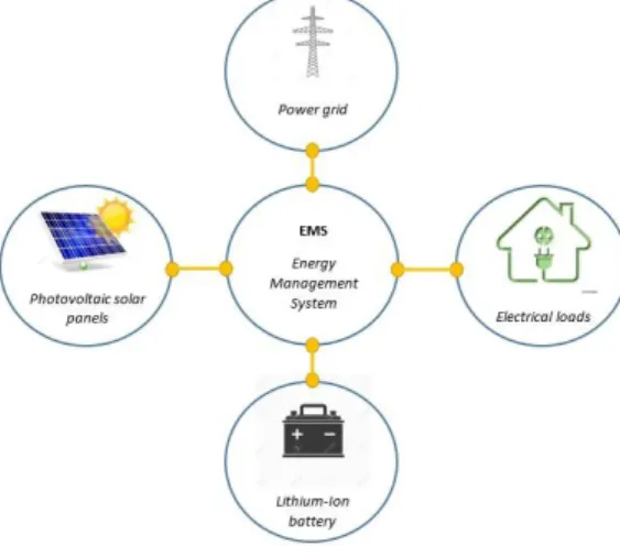
will make it possible to increase the self-consumed energy but also to mitigate the power variability on the grid due to the intermittent of renewable energies. In our case, an eco-district in Toulouse was considered, composed of twenty houses of 100 m2_{heated by heat pumps and equipped with} roof-mounted PV system and second life batteries. This microgrid is plugged into the electricity grid. The production and consumption data are normalized from the Homer software (synthetic data): production data for 1 kWp of photovoltaic panels in Toulouse and consumption data for a normalized residential type profile for an average daily consumption of 1 kWh. On the consumption profile, a peak in the evening is observed, when the solar panels no longer produce. Hence, in order to reduce the peak energy consumption on the grid, a storage is coupled on the microgrid (Fig. 1).

Fig. 1: Global synoptic of the microgrid

The grid service applied to the microgrid is related to the self-consumption with resale of the energy surplus as proposed in French policies for small producers (36 kWp<Pp<100 kWp). It is here possible to obtain a total 5-year photovoltaic investment bonus of 0.09 €/Wp paid annually over five years and to sell the surplus energy produced at a rate set at 0.06 €/kWh [1]. The energy purchased on the electricity grid will be invoiced at the standard Electricity of France (EDF) price of 0.147 €/kWh.

𝐶𝑜𝑠𝑡 = 𝐸𝑜𝑢𝑡 ⋅ €𝑜𝑢𝑡− 𝐸𝑖𝑛 ⋅ €𝑖𝑛 (1)

With:

 Eout energy injected into the electrical grid (kWh).

 €out grid injection price of energy at 0.06 €/kWh.

 Ein energy extracted from the electrical grid (kWh).

 €in purchase energy price at 0.147 €/kWh.

The objective of the microgrid is firstly to satisfy the needs of energy consumers by limiting grid impact. The Energy Management Strategy (EMS) is built on simple heuristic. The issue is to use the energy produced as much as possible to avoid buying it at more expensive price or to sell it at a low price. The battery is used as soon as consumption is different from production in order to readjust the production-consumption balance. In case of underproduction, the battery provides the missing energy until it reaches its minimum of State Of Charge (SOC), in which case it is necessary to buy energy from the electricity grid. In a case of overproduction, firstly, the battery is charged and when it reaches the maximum SOC, energy will be injected into the grid. Given photovoltaic production data (PPV) and consumption data (Pload) seen as the program inputs, the EMS will allocate power flows in the different devices of the microgrid while monitoring the state of the battery [i.e. both (SOC) and state of health (SOH)] to estimate the power (Preal) that it can actually deliver. In order to do this, it is necessary to have a battery model, which is presented in the next section.

𝑃𝑔𝑟𝑖𝑑 = 𝑃𝑙𝑜𝑎𝑑− 𝑃𝑃𝑉− 𝑃𝑏𝑎𝑡𝑡𝑒𝑟𝑦 (2)

𝑃𝑏𝑎𝑡𝑡𝑒𝑟𝑦= 𝑀(𝑃𝑙𝑜𝑎𝑑− 𝑃𝑃𝑉 ; 𝑃𝑟𝑒𝑎𝑙) (3)

With:

 Pload and PPV >0.

 Pgrid and Pbattery can be positive or negative : <0 in charge et >0 in discharge.

(3)

The objective of the techno-economic model developed on Matlab from previous works [2-4] is to simulate a microgrid, including a second life lithium-ion (Li-ion) battery over a long period of time (typically the microgrid lifecycle) to get technical and economic data. In order to do that, the tool proceeds in four steps: simulation data entry, technical simulation, economic simulation and results display. Table I presents the values of parameters set during the simulations.

Table I: Parameters set

Simulation time

Step time for technical simulation

Step time for economic simulation PV investment bonus Purchase energy price Redemption price of energy 30 years 10 minutes 1 year 0.09 €/Wp 0.147 €/kWh 0.06 €/kWh

B) Lithium-ion battery model

Storage elements are characterized by their energy density (Wh/kg) and power density (W/kg). Li-ion batteries have the advantage to have a higher energy density and power density than lead or nickel-based batteries. Li-ion technology has developed strongly since the 1980s with the first commercialization in 1991 by Sony Energitech. In this part, the modelling of Li-ion battery will be discussed. Two models [5] are used (Fig.2) to design the battery as well as possible:

 A behavioural model. It simulates the electrical behaviour of battery in order to calculate its SOC and its voltage. Hence, with these values, the EMS can control the battery level before allocating the power flows in the microgrid.

 An ageing model, which allows estimating the degradation of the battery in order to get its SOH.

Fig. 2: The battery model.

B.1) Characteristics of the tested battery

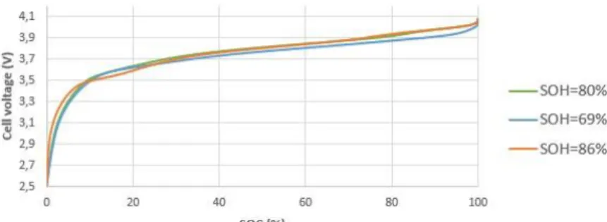
As part of this study, we focused on second-life Carbon - Lithium Manganese Oxide (C-LMO) Li-ion batteries from electric vehicles. It is composed of a negative carbon electrode (graphite) and a positive electrode based on spinel structures: lithium manganese oxide (LMO) using mainly manganese, which has the advantage of being available in large quantities [6]. The Aging model is based on the cycle to failure curve for a temperature at 25°C and a C/2 discharge regime. It allows to know, for a given depth of discharge (DOD), the maximum number of equivalent maximum cycles. To obtain the parameters of the behaviour model, C/2 discharge characteristics (Fig. 3) was used for three SOH: 86%, 80%, 69%.

Fig. 3: Discharge curves at C/2 for different SOH

As the electric vehicle market is particularly recent, many batteries are now arriving for recycling at high SOH levels (between 80 and 90%) due to accidents or manufacturer returns. Therefore, in this study, a high initial SOHini in second life was taken at 90%. In the future, this SOH before recycling will drop to the expected 65%. Table II presents the battery’s parameters set.

(4)

Table II: Battery parameters set

SOCmin SOCmax SOHini SOHlim Vmin Vmax C-ratemax Qnom

10 % 90 % 90 % 45 % 2.5 V 4.1 V C/2 50 Ah

B.2) The behaviour model

There are several types of battery models in the literature [3] [6]:

 Mathematical models (neural networks, fuzzy logic).

 Electrochemical models.

 Equivalent electrical circuit models.

For our application with a systemic vision of a microgrid, electrical circuit models seem to be the most suitable because they offer a good compromise between computation time and accuracy [2].

B.2.1) Description of the Tremblay-Dessaint model

The Tremblay-Dessaint [2-4] [7-8] model (Fig. 4) is a quasi-static model where voltage and current are separated. It comes from Shepherd’s work in 1965 and describes the battery operation from the discharge curve (taking into account the evolution of the voltage depending on the SOC) knowing the current and the SOC.

Fig. 4: Equivalent electrical circuit.

In the case of our study, the calculation time step is large enough Δt=10 min, it is possible to neglect the filtering effect modelled by C2 [2], so we take i instead of i*. The expressions of the Tremblay-Dessaint model can be written according to the SOC where the OCV is the open circuit voltage of the cell battery and R the resistive terms [8]:

OCV (SOC) =𝐸0+𝐴𝑒−𝐵𝑄𝑛𝑜𝑚(1−𝑆𝑂𝐶)−𝐾𝑄𝑛𝑜𝑚( 1 𝑆𝑂𝐶− 1) (4) 𝑉𝑏𝑎𝑡 𝑖𝑛 𝑑𝑖𝑠𝑐ℎ𝑎𝑟𝑔𝑒= 𝑂𝐶𝑉(𝑆𝑂𝐶) −𝑅1 𝑖 −𝑅2𝑖 ( 1 𝑆𝑂𝐶) (5) 𝑉𝑏𝑎𝑡 𝑖𝑛 𝑐ℎ𝑎𝑟𝑔𝑒 = 𝑂𝐶𝑉(𝑆𝑂𝐶) −𝑅1 𝑖 −𝑅2𝑖 ( 1 1.1−𝑆𝑂𝐶) (6)

It is necessary to identify the Tremblay-Dessaint parameters model [E0, A, B, K, R1, R2] from a cell characteristics.

B.2.2) Evolution of parameters with ageing

It is important to investigate the evolution of the parameters of this model with ageing in order to modify the parameters of the Tremblay-Dessaint model. In the literature [9], OCV characteristics according to the SOC for (C-LMO) cells for different SOH are presented in Fig. 5.

(5)

It can be noted from Fig. 5 that, for a given SOC, the value of the OCV remains almost identical regardless of the SOH of the cell. Therefore, in the OCV equation, it is assumed that the parameters [E0, A, B, K] remain constant despite ageing.

However, ageing mainly affects two factors: a decrease in capacity and an increase of the internal resistance of the battery as shown in Fig. 6 [6]. Hence, the SOC takes into account the ageing of the battery cell with the value Qdeg which represents the real capacity of the cell at a given instant tk:

𝑆𝑂𝐶𝑘+1= 𝑆𝑂𝐶𝑘−

∫𝑡𝑘+1𝑖 𝑑𝑡 𝑡𝑘

𝑄𝑑𝑒𝑔 𝑘

(7)

Fig. 6: Evolution of capacity and internal resistance with ageing [6]

In order to take into account the increase on internal resistance with ageing, it will then be necessary to modify the value of the internal resistance R1 in the Tremblay-Dessaint model. From the observations

of the work carried out by Akram Eddahech [6], a linear evolution of the internal resistance seems more suitable for low temperatures.

B.2.3) Method for identifying parameters

In order to identify the parameters of the Tremblay-Dessaint model [E0, A, B, K, R1, R2] of the cell, an optimization algorithm is required: the non-linear least squares method was used. It consists in minimizing the error between the experimental data (yi) and the model (f).

S(θ) = ∑𝑁𝑖=1(𝑦𝑖− 𝑓(𝑥𝑖 ; 𝜃))2 (8)

With in our case:

 N: number of cell voltage measurement points.

 xi: inputs of the Tremblay-Dessaint model at point i, namely the current and the SOC.

 : unknowns of the Tremblay-Dessaint [E0, A, B, K, R1, R2].

For the identification process, we decided to use the following method. First, the OCV parameters were obtained from OCV characteristic (Fig. 5). Then R1 (with an ageing law) and R2 parameters were determined from discharge curves (Fig. 3).

Table III presents the accuracy performance of the model for the discharge curves studied (SOH=86%, 80% and 69%).

Table III: Errors between model and data

SOH=86% SOH=80% SOH=69%

Mean-squared error 0.60 mV 0.79 mV 0.86 mV

Average relative error 0.52 % 0.45 % 0.5 %

B.3) The ageing model: “exchangeable energy model”

The ageing model allows to estimate the SOH of the battery cell. For batteries oriented energy, the SOH can be calculated as the ratio between the actual capacity of the battery and its maximal capacity. There are two types of ageing that occur in the battery operation [6]:

(6)

 Calendar ageing which corresponds to the cell performance degradation over time when the battery not operates.

 Ageing in cycling which refers to the cell performance degradation when a battery current circulate in the battery.

In the literature, there are three types of ageing models: physical, mathematical or fatigue models. In our case, with a systemic approach of a microgrid, the fatigue models seem to be the most adapted because they present a good compromise between calculation time/accuracy. Hence, the issue was simplified by considering the “exchangeable energy model” which consists in calculating the battery degradation as a function of the amount of energy (in charge and discharge) that the battery can exchange with the system throughout its life (between SOHini and SOHlim [2-3]. This maximum amount of exchangeable energy is estimated [2-3] from the "cycle to failure" curve where it is possible to read the maximum number of cycles according to the chosen discharge depth:

𝐸𝑒𝑥𝑐ℎ 𝑚𝑎𝑥 = 2. 𝑁 𝑐𝑦𝑐𝑙𝑒𝑠 𝑚𝑎𝑥(𝐷𝑂𝐷𝑐ℎ𝑜𝑠𝑒𝑛 ). 𝐷𝑂𝐷𝑐ℎ𝑜𝑠𝑒𝑛. 𝐸𝑖𝑟𝑎𝑡𝑒𝑑 (9)

With:

 Erated: rated energy of the battery for SOHini.

 DODchosen desired depth of discharge for the battery cycle (between 0 and 1).

 Ncycles max: maximum number of cycles for a DOD set to DODchosen.

 Eexch max: maximum amount of energy that can be exchanged by the battery during a certain period of its life (between SOHini and SOHlim).

Finally, the SOH is determined at the next step from the energy exchanged during a time step according to the formula below:

𝑆𝑂𝐻𝑘+1= 𝑆𝑂𝐻𝑖𝑛𝑖+ 𝑆𝑂𝐻_𝑙𝑖𝑚−𝑆𝑂𝐻_𝑖𝑛𝑖 𝐸_{𝑒𝑥𝑐ℎ 𝑚𝑎𝑥} ∗ ∑ |𝐸𝑒𝑥𝑐ℎ (𝑖)| 𝑘+1 𝑖=1 (10) With |𝐸𝑒𝑥𝑐ℎ| = ∫ |𝑃𝑏𝑎𝑡 (𝑡)| 𝑡+𝛥𝑡 𝑡 𝑑𝑡 (11)

C) Economic Model

In order to assess a techno economic analysis, it is necessary to calculate economic indicators to estimate the whole cost of the microgrid over its life cycle (i.e. the NPV, for Net Present Value is defined below). This latter is based on cash flows, noted Fm for the year m. Cash flows take into account the incomes

due to the chosen self-consumption strategy (𝑐𝑓𝑔𝑟𝑖𝑑 𝑚 ) with resale of the power surplus for small

producers (see part II in the case of French policies), to which the operating and maintenance costs (OPEX) must be deducted. To adjust the elements to the current value of costs for the year under consideration, it is required to multiply by (1+e)m_{with e the inflation rate.}

𝐹 𝑚 = 𝑐𝑓𝑔𝑟𝑖𝑑 𝑚 − 𝑂𝑃𝐸𝑋𝑚 (12)

𝑐𝑓𝑔𝑟𝑖𝑑 𝑚 = (𝐸𝑜𝑢𝑡 ⋅ €𝑜𝑢𝑡− 𝐸𝑖𝑛 ⋅ €𝑖𝑛) ⋅ (1 + 𝑒)𝑚 (13)

𝑂𝑃𝐸𝑋𝑚 = (1 + 𝑒) 𝑚⋅ 𝑂𝑃𝐸𝑋 (14)

In our case, the CAPital Expenditure (CAPEX) takes into account the investment related to the photovoltaic production source CAPEXPV (development costs, purchase and delivery of equipment (solar panels, inverters, etc.), installation and connection) and that concerning the means of storage CAPEXBAT. The investment is considered to be fully paid the first year (no loan). To stay in a simple economic vision, investment costs were estimated in €/kWp for the photovoltaic production source and in €/kWh for the battery system. Regarding the OPEX, there are estimated as percentage rOM each year of the initial CAPEX investment. However, to be more precise, the OPEX of the battery is divided into two parts: a fixed part which will be a percentage of the CAPEX each year of the battery life and a variable part to take into account the extra cost when replacing the battery. The variable part is expressed as the cost (CAPEXbat – rRep . nbmodule €) by replacing of all the batteries with rRep the cost (€) that can be saved per module compared to the initial price of the battery (recovery of certain elements, in particular electronic devices such as BMS).

In a project, the net present value (NPV) is used to account for the overall cost of the microgrid over its lifetime by integrating its energy management strategy and its environment (solar irradiation, grid

(7)

policies and rates). To do this, year by year, the cash flow is discounted to current value using the actual discount rate d [2].

𝑁𝑃𝑉 = −𝐶𝐴𝑃𝐸𝑋 + ∑ 𝐹𝑚 (1+𝑑)𝑦𝑒𝑎𝑟 𝑁

𝑦𝑒𝑎𝑟=1 (15)

Table IV: set of economic parameters

Inflation rate Discount rate PV CAPEX

OPEX for PV Battery CAPEX

OPEX for Battery e = 2 % d = 3 % Cinv PV =

1.2 €/Wp of CAPEX PV rOM PV = 2.5 % / year

cinv bat =

200€/kWh Fixed part : rCAPEX battery / year OM bat = 2% of

Variable part : rRep = 70€ saved / module replaced In the economic model implemented to analyse the microgrid performance, the objective is to self-consume as much energy as possible (self-consumption case). That is why the microgrid does not allow to earn money. It is more convenient to compare the case of the microgrid with a “reference case” for which 100% of consumed energy is purchased from the electricity grid at a fixed price. The interest is to analyse if it is economically more profitable to create your microgrid (with corresponding investments and to self-consume your own energy as much possible) than to purchase energy from the grid at fixed price. In our analysis, the first key indicator will be the “relative NPV” (ΔNPV) which is the difference between the microgrid NPV (including a certain sizing of both the solar array and the storage device) and a reference system NPVref, which will obviously be negative, which would include neither storage device nor PhotoVoltaic (PV) source and which would lead to purchase the total consumed energy to the grid by considering the actual purchase rates €in. Thus, the microgrid is profitable if:

𝛥𝑁𝑃𝑉 = 𝑁𝑃𝑉 − 𝑁𝑃𝑉𝑟𝑒𝑓 > 0 (16) 𝑊𝑖𝑡ℎ 𝑁𝑃𝑉𝑅𝐸𝐹= ∑ −𝐸𝑐𝑜𝑛𝑠𝑢𝑚𝑒𝑑 . €𝑖𝑛 (1+𝑑)𝑦𝑒𝑎𝑟 𝑁 𝑦𝑒𝑎𝑟=1 (17)

To take account for the profitability of the microgrid in relation to the reference case, two typical economic indicators are calculated: the return on investment time (ROIT) and the profitability index (PI). The ROIT (years) represents the time from which the invested capital is recovered, i.e. when the cumulative NPV of the microgrid becomes higher than that of cumulative reference NPVref. The PI is the ratio between the financial gain at the end of the migrogrid lifetime and the CAPital Expenditure (CAPEX):

𝑃𝐼𝑟𝑒𝑓 = 𝛥𝑁𝑃𝑉

𝐶𝐴𝑃𝐸𝑋 (18)

D) Some analysis results and discussion

With the emerging smart grids integrating intermittent renewable power sources, new pricing policies would appear to encourage renewable energy plants (solar, wind) coupled with storage to limit the use of the grid. As energy indicator, we know the “degree of autonomy” defined as the ratio between the energy produced and the energy consumed. But this latter indicator does not differ depending if the consumption takes place during production or outside production phases, thus neglecting the constraints of the grid (line congestion, etc). To quantify more conveniently the level of grid constraint, a new indicator called “degree of grid usage” (DGU) is defined as the ratio at each time step between the average grid energy (whatever if it is injected or extracted) and the energy consumed (excluding battery consumption):

DGU (in %) = 100*𝑀𝑒𝑎𝑛 𝑘=1𝑁 (

𝐺𝑟𝑖𝑑 𝑒𝑛𝑒𝑟𝑔𝑦 𝑘

𝐶𝑜𝑛𝑠𝑢𝑚𝑒𝑑 𝑒𝑛𝑒𝑟𝑔𝑦 𝑘)

(19)

with k the step time and N the number of points.

The issue about this indicator is linked with the fact that grid power must be balanced in both ways, over production as well as over consumption

A first interesting analysis aims at assessing both the peak power of the photovoltaic installation and the total stored energy for the Li-ion battery with respect to the policies and grid services with that

(8)

microgrid. It is necessary to look for the best configuration in order to maximize the ΔNPV or to minimize the DGU. To do this, the mapping of figure 7 allows having a trend on the profitability and the grid usage according to the investments (sizing of devices). The following maps are obtained with Enom (battery sizing) on the x-axis and PPV (solar panels sizing) on the y-axis. The scale color represents the value of ΔNPV on the left and DGU on the right with in yellow the highest values and in blue the lowest values.

Fig. 7: Maps of the ΔNPV and the DGU versus both device sizing

It can be noted that the pairs with the best ΔNPV (yellow part) are located at high installed peak power and with a storage capacity of less than 400 kWh with assumptions made in the model. Indeed, with this strategy, the optimal point to maximize ΔNPV is: ΔNPV=199k€ for PPV=100kWp and Enom=198kWh. With this sizing of photovoltaic panels and based on the assumptions taken from the model, a case with storage is more profitable than a case without storage. Thus, with such grid policies and economic assessments, there is a benefit with storage by using the energy produced during the day and by postponing it to the evening to avoid buying expensive energy from the electrical grid. Even if the DGU (equal to 71.3% for the techno economic optimum point) is smaller than if the consumers would buy all the energy needs, this parameter may be improved with other battery sizing making the microgrid more and more autonomous. Looking at the Degree of Grid Usage (DGU) map (on the right), we notice that the optimal point in terms of DGU is: DGU=37%, obtained for PPV=68kWp and with the maximal storage capacity Enom on this map: Enom=798kWh. But the ΔNPV= -4 227 € is here really negative with such a storage device: we can have here an “idea of the cost for full autonomy with stand alone microgrids”. With this funding strategy, both indicators (ΔNPV and DGU) are not compatible (the yellow area on the left does not overlap the blue area on the right).

D.1) Analysis at the maximum ΔNPV point

D.1.1) Analysis of the battery performance degradation over the life cycle

Thereafter, the techno-economic analysis is carried out for the optimal sizing in terms of ΔNPV (i.e. PPV = 100kWp and Enom=198kWh). For this simulation, the battery model parameters change with the battery ageing (R1 and Q). Looking at the evolution on the battery State Of Health (SOH) over the full lifetime of the microgrid (in our case 30 years), it appears that it is not necessary to change the battery as the SOH reaches 59% after 30 years. From an economic point of view, the microgrid costs more money each year than it brings us (Net Present Value (NPV)= -333.3k€<0). However, analysing the relative evolution of the cumulative ΔNPV observed by comparing the net present value of the microgrid with that of the reference case (with neither PV nor storage), the obtained Return On Investment Time is less than 12 years meaning that the microgrid costs less than buying all energy from the grid. Compared to this reference, the microgrid investments will be profitable and will save 199k€ after 30 years.

D.1.2) Comparison of analysis with and without battery performance degradation

With the same optimal sizing, it is possible to compare the previous results with the ones obtained without taking into account the degradation of battery performance due to the ageing (capacity and power losses), i.e there is no loopback of SOH on behavioural model parameters (R and SOC). In this latter case, the ageing model only allows to estimate the State Of Health (SOH) in order to calculate the cashflow (taking into account the cost of battery changes when they take place). The comparative analysis between the two cases are below.

(9)

ΔNPV (k€) NPV (k€) SOH end (%) Qth cell (kAh)

Without degradation 208.9 -323.3 55.5 534

With degradation 198.9 -333.3 59.2 477.6

Error (%) 5 3 6 12

After 30 years, without considering the degradation of battery performance, it can be observed that more ampere hours (Qth cell) are exchanged with the storage device. Indeed, the battery without accounting the degradation (with a constant capacity) is able to maintain the exchanged energy during cycle as in its initial conditions. This will result in a lower SOH than if the degradation is taken account.

The relative error between both cases (with and without accounting the degradation) is significant on technical data: 6% on SOH and 12% on Qth (Ampere-hour exchanged by the battery). However, at the economic level, the error is decreasing with only 3% on NPV and 5% on ΔNPV.

Setting the simulation time at 20 years, the error on NPV is reduced by half. Let notice that taking into account ageing on the battery's behaviour improves accuracy of analysis but increases the computation time.

D.2) Discussion

The previous results show a favorable trend towards the development of renewable sources (solar PV) and the implementation of storage devices in microgrids. This trend exists not only from an economic point of view (i.e. the ΔNPV is more important than without storage at the optimal sizing point) but also from a technical point of view (limitation of grid usage with a smart energy management, etc.). However, these results should be taken with some caution because we have placed ourselves in a very particular case study, dealing with an eco-neighbourhood with an Electricity of France (EDF) contract for the resale of the power surplus. The techno-economic model is built from hypotheses and simple models. In our case study, it is assumed that the contract for reselling the surplus with EDF remains valid for the entire life (30-years) of the microgrid (roughly corresponding with the solar panel life time), whereas it is a 20-year contract. In our model, the parameter set at the beginning of the simulation will remain the same during the 30 years, being just subject to the inflation rate (set here at 2%). However, it is obvious that certain parameters, such as the purchase price of energy, are likely to increase significantly in the next thirty years. It is thus difficult to predict economic parameters over a long period of time. For this reason, a sensitivity analysis was carried out to determine the parameters that have the greatest impact on the final ΔNPV. The sensitivity analysis revealed that the parameters which have a strong influence on ΔNPV are the inflation rate, the discount rate and the purchase price of energy from the grid. In addition, the cell temperature is considered constant around 25°C because of the low current regimes (C/2) recommendation to limit battery heating and therefore ageing. It is not necessary here to change the batteries for 30 years because the second life of the batteries was here started at high initial State Of Health (SOHini = 90%). Moreover, in our model, the efficiency of power electronic devices are not taken into account and it is assumed that a perfect balancing of the cells was performed (SOH of a cell = SOH of the battery pack) thanks to the balancing system of the Battery Management System (BMS). However, in reality, there can be a significant dispersion of the capacity of the different cells constituting the battery, all the more for second life batteries (with different first lifes).

In this work, the exchangeable energy model has been retained to take into account the battery ageing during cycling by neglecting the calendar ageing. Two different approaches were discussed: the first one was to consider that the ageing model has an impact only on economic indicators via the estimation of the battery SOH without considering the degradation of battery performance. Reasoning on global systems, the objective here was to estimate the qualitative trends of ageing in order to know which parameters were the most sensitive with the greatest impact on life expectancy. The second approach has considered that the ageing model has an impact, not only on economic indicators via the SOH, but also on technical performance (by coupling ageing effects on certain battery model parameters: R1 and Q). This approach allows to have a better accuracy on analysis but the calculation time is much more important because it is necessary to carry out the technical simulation on all years of the microgrid life. On the contrary, with the first approach, it is possible to simulate the behavior of the battery over one typical year and to consider that this year is repeated on the life time. This first qualitative analysis allows to save in computing time by going from a few minutes to a few seconds.

(10)

Conclusion

This study was essentially based on the modelling of a battery within a microgrid especially in the case of second life batteries. It provides a first simplified version of a techno-economic tool for microgrid analysis which will be developed further in the future. Such tools are needed to better understand how to improve the device sizing in microgrids, the competitiveness of battery technologies and to predict their ageing in a global system. In the particular case of second life batteries, the techno economic analysis is of prime necessity. The advantage of this tool is that it is easily scalable and allows adding quickly new features or testing different case studies.

Through this first study and with the hypotheses considered, an eco-neighbourhood composed of 20 houses was analysed and showed that it was possible to take advantage of the installation of a second-life battery both from a technical point of view to reduce grid dependence and also from an economic point of view to improve profitability. In addition, the sensitivity analysis revealed that the economic parameters having a strong influence on the profitability of the microgrid ΔNPV are the inflation rate, the discount rate and the purchase price of energy from the grid. The modeling of the second life battery includes two models: a Tremblay-Dessaint behavioral model whose parameters were identified on discharge curves of second life batteries at different SOH and an exchangeable energy ageing model (taking into account the ageing in cycling and not calendar ageing). In this work, two different approaches were processed: with and without taking into account the battery degradation on model parameters. Between the two cases, it is a compromise between precision (increase of 12% for certain technical data such as Ah exchanged) and calculation time (switch from few minutes to few seconds) that needs to be made.

For the future, the challenge is to include more complex energy management strategies, but most of all to improve the accuracy of the tool by refining hypothesis for example by taking into account the losses due to power electronics, the ageing of the various components of the microgrid (production sources, power electronics, etc.), the performance losses of batteries due to the dispersion of the cells’ capacity in a module over time, but also the uncertainty of the evolution of the economic parameters over the years. To improve these studies, it will be also necessary in the future to develop more complex and precise ageing models (e. g. electrochemical) to better take into account the phenomena occurring within second life batteries (impact on second-lifetime of SOH and resistance values at the end-of-first-life, related to first-life use).

References

[1] EDF ENR, Une prime pour encourager l’autoconsommation solaire, 10th december 2018, Electronic version:

https://www.edfenr.com/actualites/ prime-encourage-autoconsommation/

[2] Minh, Rapport de synthèse des activités de recherche au sein du Laboratoire LAPLACE dans le cadre du lot 3.5 : Optimisation technico économique, October 2016.

[3] R. Rigo-Mariani, Méthodes de conception intégrée « dimensionnement-gestion », doctoral thesis at the University of Toulouse, 2014.

[4] Andy Varais, Modèles à échelle réduite en similitude pour l'ingénierie système et l'expérimentation simulée "temps compacté": application à un micro-réseau incluant un stockage électrochimique, doctoral thesis at the University of Toulouse, 2019.

[5] Charles Delacourt, Vieillissement des accumulateurs lithium-ion dans l’automobile, Techniques de l’ingénieur re231, July 2014.

[6] Akram Eddahech, Modélisation du vieillissement et détermination de l’état de santé de batteries lithium-ion pour application véhicule électrique et hybride, doctoral thesis at the University of Bordeaux, 2014. [7] O. Tremblay et L.-A. Dessaint, Experimental Validation of a Battery Dynamic Model for EV Applications, World Electric Vehicle Journal, vol. 3, 2009.

[8] Javier M. Cabello, Battery dynamic model improvement with parameters estimation and experimental validation, University of Toulouse and National University of Rosario, 2015.

[9] Caiping Zhang, Jiuchun Jiang, Linjing Zhang, Sijia Liu, Leyi Wang and Poh Chaing Loh, A Generalized SOC-OCV Model for Lithium-Ion Batteries and the SOC Estimations for LNMCO Battery , November 2016.