HAL Id: hal-01373190
https://hal-amu.archives-ouvertes.fr/hal-01373190
Submitted on 1 Jun 2017
HAL is a multi-disciplinary open access
archive for the deposit and dissemination of
sci-entific research documents, whether they are
pub-lished or not. The documents may come from
teaching and research institutions in France or
abroad, or from public or private research centers.
L’archive ouverte pluridisciplinaire HAL, est
destinée au dépôt et à la diffusion de documents
scientifiques de niveau recherche, publiés ou non,
émanant des établissements d’enseignement et de
recherche français ou étrangers, des laboratoires
publics ou privés.
Selection of variables structured by regularization in a
multi-task framework
Antoine Bonnefoy, Ismael Ouamlil, Jean-Baptiste Veyrieras, Pierre Mahé
To cite this version:
Antoine Bonnefoy, Ismael Ouamlil, Jean-Baptiste Veyrieras, Pierre Mahé. Selection of variables
struc-tured by regularization in a multi-task framework. Conférence francophone sur l’apprentissage
au-tomatique (CAp), Jul 2016, Marseille, France. �hal-01373190�
Sélection de variables structurée par régularisation jointe dans un
cadre multi-tâches
Antoine Bonnefoy
1, Ismael Ouamlil
2, Jean-Baptiste Veyrieras
2, et Pierre Mahé
2 1Université Aix-Marseille, Laboratoire d’Informatique Fondamentale, Marseille, France.
2
bioMérieux, Bioinformatics Research Department, Marcy L’Etoile, France.
14 avril 2016
Résumé
Motivated by diagnostic applications in the field of clinical microbiology, we introduce a joint in-put/output regularization method to perform struc-tured variable selection in a multi-task setting where tasks can exhibit various degrees of correlation. Our ap-proach extensively relies on the tree-structured group-lasso penalty and explicitly combines hierarchical structures defined across features and task by means of the Cartesian product of graphs to induce a global hierarchical group structure. A vectorization procedure is then used to solve the resulting multi-task problem with standard mono-task optimization algorithms de-veloped for the overlapping group-lasso problem. Ex-perimental results on simulated and real data demons-trate the interest of the approach.
1 Introduction
Several studies have recently demonstrated the fea-sibility of predicting the antibiotic resistance of a mi-croorganism from its genome, where a good concor-dance was observed between predicted and reference resistance phenotypes, the later being determined ex-perimentally by assessing their ability to develop in presence of antiobiotic (e.g. Gordon et al., 2014). Our work is motivated by these latter proofs of concept. More precisely, starting from a large list of candidate antibiotic resistance markers extracted from microor-ganisms genomes, we aim to learn sparse predictive mo-dels of their resistance profile, that is, their resistance to several antibiotics. We target sparse models because we expect the underlying biological mechanisms to in-volve a limited number of genetic determinants, and
we want to retain some level of interpretability in the models obtained. From the statistical learning perspec-tive, we are facing a multi-task learning issue, where the tasks —antibiotics in our case— can exhibit va-rious degrees of correlation, since in practice we may be interested in several groups of antibiotics targeting distinct resistance mechanisms. Moreover, as it will be described in Section 6, the candidate genetic markers we consider can naturally be categorized in a hierar-chy, organized for instance as genes and mutations wi-thin genes. Taking into account both of these struc-tures, across tasks, and markers, as prior knowledge for learning may lead to better models. On the one hand, multi-task learning has been shown to be relevant in va-rious situations to consider dependency between tasks. In particular, in cases where tasks present several de-grees of similarity, Kim and Xing (2010) proposed an approach to leverage a hierarchical structure encoding the similarity between tasks to learn sparse multi-task models. The method is based on a specific group-lasso penalty involving tree-structured overlapping groups, and can be seen as an extension of a common multi-task approach consisting in learning jointly several models sharing the same support (Obozinski et al., 2008). On the other hand, considering the categorization of the features can lead to a principled strategy to include features in the model, that can be beneficial in terms of performance and interpretability (Zhao et al., 2009; Jenatton and Mairal, 2010; Jenatton et al., 2011).
We propose in this work to take into account both structures to define a joint regularizer. By doing so, we aim to impose a hierarchical constraint on the support of each model, while maintaining the flexibility of the structured multi-task approach. We introduce for this purpose a new group-lasso regularizer explicitly combi-ning the input and output hierarchical structures, and
propose a simple vectorization procedure allowing to cast this multi-task problem into a mono-task one. Ex-perimental results on simulated and real data demons-trate the interest of the approach.
2 Background on tree-structured
group lasso
In this section, we introduce the notations that will be used throughout the document and provide some background about the tree-structured group-lasso pe-nalty, and its application to structured variable selec-tion and to multi-task learning.
2.1 Notation
The notation are given for any (m, p) 2 N2. For any
vector w 2 Rp, the i-th component of w is denoted
by wi, and for any q 1, kwkq = (Ppi=1|wi|q) 1/q
de-notes the `q-norm of w. For any matrix M 2 Rm⇥p
and any pair of groups (g, h) ✓ [1, m] ⇥ [1, p] we de-note the sub-matrix Mg,h = [Mi,j](i,j)2g⇥h. This
no-tation extends to any set c of couples of indices :
Mc= [Mi,j](i,j)2c. Using a dot in this notation means
that the corresponding matrix dimension is not sub-sampled, i.e. Mg,· = [Mi,j](i,j)2g⇥[1,p]. This notation
extends to vectors wg = [wi]|i2g. The set of vertices
and edges of a tree T are denoted as V(T ) and E(T ), respectively.
2.2 Tree-structured group lasso for
structured variable selection
We first consider a mono-task setting where we want to learn a linear model, defined by a vector w 2 Rp,
from observations (xi, yi)
2 Rp
⇥ Y, for i = 1, ..., n, where Y = R in a regression setting and Y = {+1, 1} for binary classification. The p input features are as-sumed to be organized in a directed rooted tree T : each feature is affected to a single node of the tree, which can be either an internal or a leaf node. For each node v 2 V(T ) we denote F(v) ✓ [1, · · · , p] its set of affected features. {F(v)}v2V(T ) is then a partition of
[1, . . . , p]. Each node v of the tree T induces a group gv defined as the set of features affected to v and its
descendants. Letting D(v) be the set of children of the node v 2 V(T ), the group gv is formally defined as :
gv =F(v) [ 8 < : [ u2D(v) gu 9 = ; (1)
This procedure therefore defines a hierarchical and overlapping set of groups, a group defined at a given node of the tree —except the root— being included in the groups of its ancestors, which can then be used to define a group-lasso penalty
⌦I(w) =
X
v2V(T )
⌘v||wgv||q. (2)
The parameter ⌘v allows to control the penalization of
the group gv and q is usually set to 2 or to +1, (Zhao
et al., 2009; Jenatton et al., 2011).
The group-lasso penalty has the effect of setting to zero entire groups of variables, and the hierarchical de-finition of the groups leads to the following effect : a group can only be selected provided that all its ances-tors are selected as well, or, equivalently, any group is set to zero together with its descendants. As a result, this penalty imposes a hierarchical constraint on the support of the model : if variables are affected to inter-nal nodes of the tree, they enter the model whenever one of their descendants is selected.
Remark. This hierarchical group structure extends straightforwardly to a forest of trees. It only requires to connect all the roots to a newly added – global – root with no affected features and a weight set to zero.
2.3 Tree-structured group lasso for
multi-task learning
In a multi-task setting, we want to learn T linear models, defined by vectors w1, ..., wT 2 Rp, using
multi-task observations (xi,
{yi
1, ..., yiT}) 2 Rp⇥YT, for
i = 1, ..., n. An early approach to learn sparse multi-task models defined the following penalty :
⌦S(W) = p
X
j=1
||Wj,·||q, (3)
where W = [w1, ..., wT]is a p⇥T matrix in which each
column corresponds to a model (Tropp, 2006; Obo-zinski et al., 2008). This penalty induces sparsity on W at the row level, hence has the effect of grouping features across tasks : whenever a feature is selected, it is selected simultaneously for all models at the same time. While this is a natural consideration for strongly related tasks, it may not be appropriate to jointly learn tasks exhibiting various degrees of similarity. In such a case, indeed, it may be expected to select globally more features than required individually for each task. Kim and Xing (2010) proposed to extend this approach by
considering a hierarchical structure reflecting the de-gree of correlation between tasks. A hierarchical group-lasso penalty is then defined in the same manner as in the previous section, and the global lq penalty defined
at the row level in (3) is replaced by the corresponding group-lasso penalty : ⌦O(W) = p X j=1 X v2V(T ) ⌘v||Wj,gv||q. (4)
Each feature is therefore penalized according to this group-lasso penalty, defined across tasks, which has the effect of inducing sparsity also within rows of W. A feature is therefore not systematically introduced in all models, which allows to control the inclusion of a given feature in multiple models, according to the relatedness of the corresponding tasks. Strongly related tasks can therefore be enforced to share a large fraction of their supports, while allowing them to maintain their own specificity. Conversely, tasks showing a lesser level of correlation can still be learned jointly, with a lower incentive to share common variables. The definition of the weights ⌘v is critical in this respect, and will be
further discussed in Section 4.3.
3 A joint input/output
regulari-zation method
The problem of combining input and output struc-ture has been addressed by Lee and Xing (2012) and Chen et al. (2012) who proposed joint regularizers de-fined as the sum of input and output regularizers. In this section, we propose an alternative definition that combines the input and output structures into a global one by means of the Cartesian product of graphs. Since this construction takes into account the coupling effect between the input and output structures, we shall re-fer to it as the coupled input/output tree-structured group lasso regularization, as opposed to the decou-pled approaches proposed by Lee and Xing (2012) and Chen et al. (2012). The two following sections respec-tively define this coupled approach and point out its advantages with respect to the decoupled one.
3.1 Definition
Given two hierarchical structures TI and TO
res-pectively defined across features and tasks, toge-ther with their associated sets of groups {gu}u2V(TI),
{gv}v2V(TO) defined according to (1) and
correspon-ding weights {⌘u}u2V(TI), {⌘v}v2V(TO), we define the
□
=
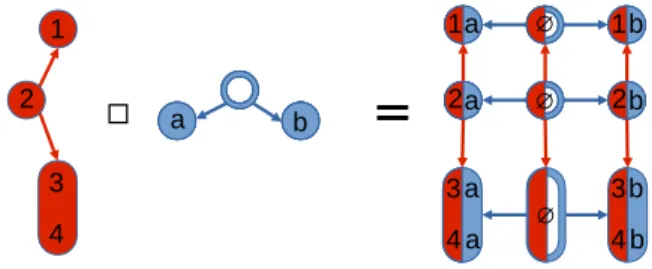
1 2 3 4 a b 2 3 4 1 2 3 4 1 a a a a b b b b ∅ ∅ ∅Figure 1: Cartesian product of tree. Each feature – integer– and task –letter– is associated to a node of the input and output tree structures, respectively. The DAG resulting from their Cartesian product is shown on the right.
coupled input/output tree-structured regularizer as : ⌦I⇤O(W) = X u2V(TI) X v2V(TO) ⌘u⌘vkWgu,gvkq. (5)
This overlapping group-lasso regularizer involves |V(TI)|⇥|V(TO)| groups, each group of the input
struc-ture defining as many groups as the output strucstruc-ture contains. This set of groups can be embedded in a unique hierarchical structure based on the Cartesian product of the input and output trees, as we now des-cribe.
Definition 1 (Product graph of hierarchical-tree structures). Given two trees TI and TO, we define
their Cartesian product TI⇤TO following the usual
definition in which V(TI⇤TO) = V(TI) ⇥ V(TO) is
the set product of V(TI)and V(TO), and two vertices
(u, v), (u0, v0)2 E(T
I⇤TO)are connected if either u =
u0 and (v, v0)2 E(T
O), or v = v0 and (u, u0)2 E(TI).
For a given vertex w = (u, v) 2 V(TI⇤TO), we define
its weight ⌘w as ⌘u⇥ ⌘v, and its set of associated
fea-tures F((u, v)) ✓ [1, · · · , p]⇥[1, · · · , T ] as F(u)⇥F(v). Definition 1 is illustrated in Figure 1. The Carte-sian product of two trees is a Directed Acyclic Graphs (DAG). A hierarchical group structure on TI⇤TO can
therefore be defined according to (1). We can now state the following result, whose proof is post-poned to Ap-pendix A.
Proposition 1. Let TI and TO be two trees and
TI⇤TO their Cartesian product according to Definition
1. Let {gu}u2V(TI), {gv}v2V(TO) and {gw}w2V(TI⇤TO)
be their hierarchical sets of groups defined according to (1). Then, for any w = (u, v) 2 V(TI⇤TO), we have
g(u,v)= gu⇥ gv.
With this property in hand, we can finally state the following result.
Proposition 2. The regularization defined in (5) is equivalent to a hierarchical group-lasso regularization on groups defined on the product graph TI⇤TO :
⌦I⇤O(W) = X u2V(TI) X v2V(TO) ⌘u⌘vkWgu,gvkq (6) = X w2V(TI⇤TO) ⌘wkWgwkq. (7)
Démonstration. This result follows directly from Pro-position 1 by noting that the set of vertices of V(TI⇤TO) is equal to V(TI)⇥ V(TO), hence that the
terms of the double sum over V(TI)and V(TO)can be
evaluated by summing over V(TI⇤TO). The result is
obtained by the definition of ⌘w as ⌘u⇥ ⌘v.
The following section discusses the effects of the pro-posed regularization with respect to that introduced in Lee and Xing (2012).
3.2 Benefits
As mentioned previously, Lee and Xing (2012) and Chen et al. (2012) proposed decoupled joint in-put/output regularizers defined as the sum of input and output regularizers. In particular, the definition consi-dered in Lee and Xing (2012) is based on a overlapping group-lasso penalty hence bears strong similarity with the one proposed in the previous section. Using the notations introduced previously, it writes as :
⌦I+O(W) = p X i=1 X v2V(TO) ⌘v||Wi,gv||q + T X j=1 X u2V(TI) ⌘u||Wgu,j||q (8)
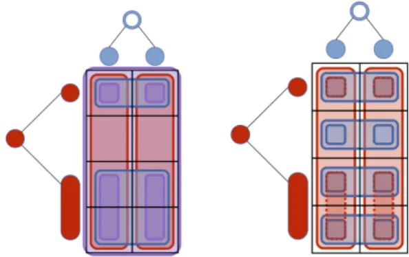
This construction has a very intuitive interpretation : it consists in repeating the output group structure for each input variable, on the one hand, and in repea-ting the input group structure for each task on the other. It is illustrated in Figure 2 using the same input and output tree structures considered to illustrate the product-graph construction.
Interestingly, we can note several differences, high-lighted in Figure 2, between the proposed coupled regu-larization (5) and the decoupled one (8). Indeed, a clo-ser look at the nature of the groups induced highlights the following disadvantages of the decoupled strategy : Redundant groups : groups associated to leaf nodes of each tree are repeated. They therefore enter twice the group-lasso definition, which adds an unne-cessary computational complexity if not properly taken
Figure 2: Comparison of the groups generated by the coupled —left— and decoupled —right— regulariza-tions, resulting from the same input and output trees.
into account.
Hierarchical and group constraints not ensu-red : the output —resp. input— group structure is re-peated for variables that are affected to internal nodes of the input —resp. output— structure. As a result, the hierarchical constraint on the support definition is not enforced anymore : a group corresponding to an internal node can be turned off without necessarily tur-ning off its descendants. Likewise, if several variables are affected to the same group, some can be set to zero without turning off the entire group.
Missing coupling effects : finally, each node in the coupled structure generates a group across tasks and features. In particular, the group defined as the entire set of input and output variables, resulting from the coupling of the two root nodes, is not included in the decoupled construction.
Remark. Several structured-sparsity problems can be seen as special cases of the coupled formulation. For instance the lasso, the simultaneous sparse coding Tropp (2006), the hierarchical sparse coding Jenatton et al. (2011) and the tree-guided group-lasso Kim and Xing (2010) can be obtained by using a trivial flat structure, defined as a collection of isolated nodes, when either tasks or features are unstructured.
4 Implementation
From a training set of multi-task observations (xi,
{yi
1, ..., yiT}) 2 Rp⇥ YT, for i = 1, ..., n, the joint
regularizer introduced in Section 3 can be used to learn multi-task models via the general formulation :
W?= arg min W2Rp⇥T n X i=1 T X t=1 l(yit, w|txi) + ⌦I⇤O(W), (9)
where l is a loss function quantifying the divergence between the prediction w|txi and the observation yit,
and is a regularization parameter controlling the trade-off between data-fitting and regularization terms. In this section we discuss implementation issues. We first introduce a simple vectorization procedure allo-wing to cast the multi-task problem into a mono-task one. We then discuss the choice of the norm to consi-der for the group-lasso penalty, and present the output groups weighting strategy.
4.1 A vectorization procedure
We now present a procedure to handle the minimi-zation problem with this joint input/output regula-rization. The base idea is to construct an equivalent vectorized version of the problem, so that its resolu-tion can be straightforwardly handled using standard proximal methods. In order to construct the equiva-lent vectorized problem, we resort to the vectorizing operator "vec" and the Kronecker product ⌦, allowing, for three matrices A, B, C, to write the following rela-tion(Petersen et al., 2006) :
vec(ABC) = (C|⌦ A) vec(B) (10) We now reformulate Problem (9) using the separa-bility of the loss function over each sample i = 1, . . . , n and task t = 1, . . . , T . Defining X = [xi]|i=1,...,n and
Y = [yt]t=1,...,T, with yt= [yit]i=1,...,n, we can write (9)
as : W?= arg min W2Rp⇥T n X i=1 T X t=1
l([Y]i,t, [XW]i,t) + ⌦I⇤O(W)
= arg min
W2Rp⇥T
nT
X
i=1
l([vec(Y)]i, [(IdT⌦ X) vec(W)]i)
+ ⌦I⇤O(W).
We then introduce the following function : ⌦vec(w) = X v2TI X t2TO ⌘v⌘tk[wi+(j 1)p]|(i,j)2gv⇥gtkq
One can easily check using the definition of vectori-zing operator that we have ⌦I⇤O(W) = ⌦vec(vec(W)).
As a result, the multi-task problem of interest (9) can be stated as an higher dimensional mono-task problem where the regularization has been modified to keep the cross-variable and cross-task structures :
w?= arg min w2RpT nT X i=1 l([vec(Y)]i, [(IdT ⌦ X)w]i) + ⌦vec(w), (11)
Remark. Note tat the manipulation of missing values is straightforward in this formulation, as it only re-quires to remove them from vec(Y) and the correspon-ding lines in IdT ⌦ X.
4.2 Choice of the group-lasso norm
Problem (11) is a special instance of group-lasso with overlapping groups. This problem is actually not easy to solve since the proximal operator of the regulariza-tion funcregulariza-tion has no analytical soluregulariza-tion. Ad hoc algo-rithms therefore have to be deployed, that depend on the choice of q and on the group structure. Fortuna-tely, an efficient polynomial time algorithm has been proposed by Mairal et al. (2011) to solve the overlap-ping group lasso for the `1-norm when the groups are
structured in a DAG. In this study, we therefore used the implementation this network-flow algorithm, which is available in the SPAMS toolbox.
4.3 Defining weights
To obtain a coherent group structure in the solution the weighting strategy is critical. Regarding the output structure, Kim and Xing (2010) proposed a data-driven strategy allowing to set the weights of the nodes so that each task is regularized equally. In this method, the output structure is built from the data by applying a hierarchical agglomerative clustering algorithm to the observation matrix Y. The result of this operation is a binary tree in which each internal node splits the tasks into two subsets. A pair of features sv and tv is
then assigned to each node v depending on its height in the tree. The value sv quantifies how its two children
subsets should be set to zero separately in the support and tv, defined as 1 sv, quantifies how they should be
kept together. The group weights are then defined as
⌘v= tv⇧v02Ancestors(v)sv, and it can then be shown that
for each leaf l of the tree, that is, for each task of the problem, we have Pv2Ancestors(l)[{l}⌘v = 1, meaning
that each task is penalized equally irrespective of its position in the tree.
Kim and Xing set the svvalue of each node according
to the normalized height of the node, leaf nodes ha-ving a height equal to zero. High nodes in the tree will therefore tend to treat their two children groups inde-pendently, hence have a lesser incentive to active them simultaneously. We refer to this strategy as absolute-height weighting and propose here a simple relative-height weighting alternative intended to better handle cases where many tasks can show very similar level of correlation, i.e. when nodes in the tree have very
si-Figure 3: Comparing the two weighting strategy on a hierarchical clustering on 10 tasks. For each node of the tree the height is given prefixed with H —except for the leaves which have 0 height—, the relative-height weight in the bottom-red rectangle and the absolute weight in the top-blue rectangle.
milar height. In this approach, we set the tv value of
each internal node as the difference between the height of its parent and its own height, and set it to 0 for the root and to 1 for the leaves. Figure 3 illustrates the weights obtained by the two strategies in a 10-task pro-blem with two groups of 5 correlated tasks. The simple intuition that large weights tend to strongly group no-des’ children may help to comprehend Figure 3. We see indeed in Figure 3 that the relative strategy tends to set bigger weights only at the top node of each of the two tasks clusters, here at height 0.42 and 0.326, which is precisely the expected behavior according to the above intuition. In contrast, we see that the nodes between the leaf nodes and these two nodes are given very small weights, and in particular smaller weights than the absolute-height strategy, meaning that they practically have no effect on the regularization. Finally, we note that the relative-height strategy regularizes tasks more homogeneously within each of the 5-task clusters, which also seems natural. As a final remark, we note that node weights could easily be used to devise a pruning strategy meant to simplify the tree-structure by removing nodes with weights smaller than a given threshold. Figure 3 suggests that such a pruning would better gather the structure of the tree if it was based on the relative height weights.
5 Simulation Experiments
We present here some simulation experiments to show the interest of our approach. We aim to evaluate the performance of the approach in terms of support recovery and denoising performance in the context of least-square regression. Our synthetic data is construc-ted as follows. Each column of the input matrix X is drawn from the centered Normal distribution N (0, In)
and normalized. The target structured and sparse ma-trix W that we seek to recover is constructed from the input tree Ti and output tree To, whose
defini-tions are given afterward. We first draw its coefficients as [W]i,j ⇠ 1 + N (0,12). We then draw random pairs
of nodes (u, v) 2 V(Ti)⇥ V(To) and set the variables
in gu⇥ gv to 0. This is repeated until less than 10%
of non-zero coefficients are remaining. We also ensure that every column of W has at least 1 non-zero coef-ficient. The matrix Y is then set as Y = XW, and each column of Y is finally corrupted some Gaussian noise to reach a given SNR level. We consider ba-lanced trees as input and output hierarchical struc-tures. A balanced tree can be defined completely by two lists : (i) a first list C that gives the number of children for each depth in the tree, (ii) a second list V that gives the number of (consecutive) variables that are affected to each node at a given depth. The in-put tree is defined as Ti :{C = [4, 3, 0], V = [0, 5, 5]},
meaning that its root has 4 children whom have 3 children each. For every child v of the root we have |F(v) = 5|, and for each grand child of the root w we have |F(w)| = 5. The output-tree is defined as To : {C = [4, 3, 0], V = [0, 0, 5]}. The problem hence
involves 80 features and 60 tasks. The input tree is assumed to be known for the estimation of W, as it represents the knowledge we can have about our fea-tures. Its weights are set to 1. The output tree, on the other hand, is obtained from Y using the clustering and weighting method detailed in Section 4.3.
The support recovery performance are measured by ROC curves which are shown in Figure 4 for two SNR values. Five regularizations strategies are considered : the proposed Coupled one, resulting from the Cartesian product of the input and output trees ; the Decoupled one that is the sum the the input-tree and output-tree regularizations ; the Input and Output regularization, taking into account only the input or the output tree structure and finally the Lasso that does not consider any structure. We observe that considering solely the output structure offers a marginal gain over the Lasso in terms of support recovery. The input structure, on
Figure 4: ROC curves of the support recovery, each marker is a given value of . The scatterplot for each regularization have been smoothed via a LOWESS re-gression (Cleveland, 1981). Note that the scale of the x-axis is linear for x 10 2and logarithmic afterwards
for better readability.
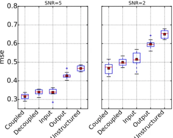
Figure 5: MSE values obtained two SNR values.
the other hand, markedly improves the results, even considered alone. Considering in addition the estima-ted output structure is beneficial only for the coupled regularization, and the improvement increases with the noise level.
To assess the denoising performance of the various regularization strategies, we repeat 10 times a process in which we generate a training dataset as described above, compute the model supports over a logarith-mic grid of values, perform a debiasing step on the resulting performance, and assess the predictive perfor-mance on independent samples, simulated by the same model. We then extract, for each repetition and each method, the smallest MSE obtained across values and show the resulting distributions in Figure 5. We
note that the coupled approach also gives better perfor-mance for the denoising task. The decoupled approach shows slightly better performance than the input only strategy for a high noise level, which may be due to a better support recovery of this method for specificity values close to one in Figure 4 for SNR=2. Further ex-periments shown in Supplementary Materials indicate that the coupled approach can further benefit from the knowledge of the actual output tree structure, highligh-ting the fact that estimahighligh-ting it accurately is important.
6 Experimental Evaluation
In this section we evaluate the relevance of the ap-proach on two real datasets involving the bacterial spe-cies Pseudomonas aeruginosa, an important human pa-thogen involved, in particular, in hospital-acquired in-fections. The first dataset is public and is described in Kos et al. (2015). It involves 390 strains characterized for three antibiotics, Amikacin, Levofloxacin and Mero-penem, belonging to three distinct families. The second dataset involves 282 strains characterized for three an-tibiotics, Meropenem, Doripenem and Imipenem, belonging to the same family —the class of penems -lactams. The level of correlation between tasks is the-refore higher in the latter dataset. In the first (resp. se-cond) database, each strain is characterized by a set of 4579 (resp. 4564) features related to 97 (resp. 95) genes involved in antibiotic resistance. These features encode the presence of absence or predefined genetic determi-nants. Most of them —4516 (resp. 4510)— correspond to the presence of a specific mutation within one of these genes, and the 63 (resp. 54) remaining ones cor-respond to the presence of some of these genes —the 34 (resp. 41) other genes being present in all the strains. These features are organized in a two-level hierarchy in which the first level corresponds to the genes. For the first dataset for instance, the root node of the tree has 97 children corresponding each to one of the genes involved in the strains characterization. Whenever a feature explicitly encodes the presence or absence of a gene —that is, for 63 of the 97 genes—, it is affected to its corresponding node. The second level corresponds to the within-gene genetic variants : each node of the first level has a various number of children equal to the number of mutations that may be observed within the corresponding gene. Finally, the output structure and associated groups weights are obtained by applying an agglomerative clustering operation on the matrix of re-sistance phenotypes, as described in Section 4.3. Note however that we consider a continuous measure of
bac-terial resistance, the Minimum Inhibitory Concentra-tion (MIC), corresponding to the smallest antibiotic concentration required to inhibit the growth of the mi-croorganism in an in vitro experiment, to build this hierarchical structure. Note also that we focus on dis-criminating between resistant and susceptible strains and discard strains of intermediate resistance.
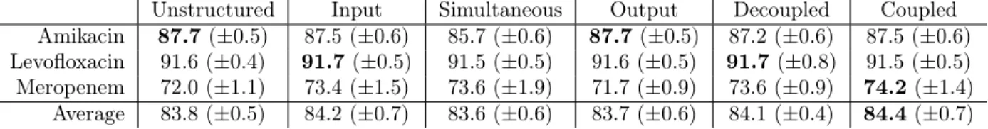
To evaluate the predictive performance of our ap-proach, we proceed by cross-validation. We consider a 10-fold cross-validation process where the regulariza-tion parameter is chosen, within each fold, by means of an internal 10-fold cross-validation process, as the value maximizing the classification accuracy over a grid of 60 candidate values. This process is repeated 5 times and is done on a task by task basis in order to stratify the folds according to the relative proportions of resistant and susceptible strains, that can vary from one anti-biotic to the other. Results are shown in Tables 1 and 2, in which we compare our approach to the four alter-native strategies described in the previous section, and to the simultaneous sparse-coding approach that forces the tasks to share the same support (Tropp, 2006).
The main conclusion that can be drawn from these tables is that the various approaches considered exhibit in general comparable performances. On the Kos data-set, in particular, all strategies provide similar perfor-mances for the Amikacin and Levofloxacin antibiotics. For the last drug, Meropenem, considering the input structure, either alone or in combination with the out-put structure, is beneficial and allows to improve the accuracy by up to 2 points. Interestingly, we note that the performances obtained on this dataset match those recently reported by Drouin et al. (2016) using a to-tally different approach, which therefore validates the use of penalized regression models in this context, as well as our list of candidate antibiotic-related genes. On the Penems dataset, the input structure also seems to have a positive impact on the classification perfor-mance. Albeit marginal (less than 1 point per antibiotic in average), the gain is systematic for the three anti-biotics. Approaches considering the output structure alone show in general lesser performance than the un-structured baseline. Consequently, joint input/output methods do not improve over the approach based on the input structure only.
We note however that although the various strate-gies lead to comparable classification performance, the nature of the supports obtained can be quite different. This is illustrated in Figure 6 that shows, for each re-gularizer, the number of active features and genes as a function of the regularization parameter. These num-bers were computed on the Kos dataset, and were
ave-raged across tasks. Note that the grid of regularization parameter is sorted in a decreasing order, and is not strictly the same across methods. It is indeed defined adaptively, starting from the minimum value of lea-ding to a non null solution. We note indeed that in terms of features, the unstructured and output strate-gies lead to the smallest supports. As can be expec-ted, the strategies taking into account the input struc-ture lead to larger supports, due to the grouping ef-fect among mutations related to a given gene. The size of the supports provided by the coupled input/output strategy is very close to that provided by the input stra-tegy, while the decoupled input/output strategy shows slightly smaller supports, probably due to the fact that the hierarchical constraint on the nature of the support is not maintained anymore. The simultaneous sparse coding strategy shows an in-between behavior. Consi-dering the number of genes activated in the supports reveals that the strategies taking into account the input structure select fewer genes than the other approaches. For practical applications, this behavior can be interes-ting to design targeted tests focusing on a more limited number of genes. Conversely, each of the unstructured, output and simultaneous strategies seems to activate a comparable number of features and genes. We note fi-nally that the simultaneous sparse-coding strategy sys-tematically activates more genes, which is probably due to the fact that the three antibiotics involved in the Kos dataset have different mechanisms of actions, hence in-volve different resistance mechanisms. As a result, since the simultaneous strategy leads to a common support across antibiotics, it is much larger than necessary for each antibiotic taken individually. The same observa-tions can be made on the Penems dataset. In this case, however, the gap between the simultaneous and the other strategies in terms of genes activated is lesser, reflecting the fact that the tasks are more correlated in this dataset.
7 Discussion
We have introduced a new multi-task regularizer combining hierarchical structures defined across fea-tures and tasks, which allows to perform structured va-riable selection when tasks can exhibit various degrees of similarity. We have demonstrated the relevance of this approach by simulation studies. Experiments car-ried out on two real datasets related to microbial anti-biotic resistance lead to mixed results, suggesting that this application does not benefit from multi-task lear-ning. Further experiments involving a greater number
Unstructured Input Simultaneous Output Decoupled Coupled Amikacin 87.7 (±0.5) 87.5 (±0.6) 85.7 (±0.6) 87.7 (±0.5) 87.2 (±0.6) 87.5 (±0.6) Levofloxacin 91.6 (±0.4) 91.7 (±0.5) 91.5 (±0.5) 91.6 (±0.5) 91.7 (±0.8) 91.5 (±0.5) Meropenem 72.0 (±1.1) 73.4 (±1.5) 73.6 (±1.9) 71.7 (±0.9) 73.6 (±0.9) 74.2 (±1.4) Average 83.8 (±0.5) 84.2 (±0.7) 83.6 (±0.6) 83.7 (±0.6) 84.1 (±0.4) 84.4 (±0.7) Table 1: Kos study. Average accuracies observed across repetitions of the cross-validation process, together with their standard deviation.
Unstructured Input Simultaneous Output Decoupled Coupled Doripenem 85.5 (±0.5) 85.9 (±0.6) 84.5 (±1.0) 83.6 (±1.2) 85.4 (±0.6) 85.2 (±0.6)
Imipenem 73.9 (±1.3) 75.5 (±1.4) 72.7 (±0.7) 73.4 (±1.0) 74.7 (±0.7) 74.9 (±0.8) Meropenem 80.2 (±0.7) 81.0 (±0.6) 81.8 (±1.1) 80.8 (±1.0) 81.0 (±1.1) 80.9 (±0.6) Average 79.9 (±0.5) 80.8 (±0.6) 79.7 (±0.8) 79.3 (±0.7) 80.4 (±0.4) 80.3 (±0.5) Table 2: Penems study. Average accuracies observed across repetitions of the cross-validation process, together with their standard deviation.
average # features vs lambda
lambda index 0 10 20 30 40 50 60 1 2 5 10 20 50 100 200 flat input simultaneous output input_output_d input_output_c
average # genes vs lambda
lambda index 0 10 20 30 40 50 60 0.5 1.0 2.0 5.0 10.0 20.0 50.0
Figure 6: Nature of the supports identified. Left and right : number of active features and genes vs regulari-zation parameter. Note that the grid of regulariregulari-zation parameter is sorted in a decreasing order.
of strains and antibiotics will be necessary to confirm the results obtained in this small scale study. This new regularizer may nevertheless be useful for other appli-cations in different domains.
We see several perspectives to this work. From the methodological standpoint, an extended empirical eva-luation would be required to assess the merits of the proposed output groups weighting strategy with res-pect to the strategy proposed in Kim and Xing (2010). We also note that we essentially chose the `1norm for
the groups for computational reasons. The overlapping `2-group lasso is indeed challenging for arbitrary
hie-rarchical graph structures, but it would be interesting to investigate whether we can exploit the particular structure of the Cartesian product of trees to devise efficient algorithms, as it is done for trees, or if we can benefit from inexact proximal methods (Schmidt
et al., 2011; Machart et al., 2012). Regarding the issue of predicting antibiotic resistance from genotypes, seve-ral natuseve-ral extensions of this work could be envisioned. We first note that finer structures could be considered to categorize the genomic features. One may for ins-tance consider the positions of mutations within the genes sequences to better account for linkage disequili-brium, which can be expected to induce local correla-tion patterns. Moreover, although we have focused in this study on a categorical resistant/susceptible phe-notype, the primary measure of antibiotic resistance is continuous. It is indeed defined as the smallest an-tibiotic concentration required to inhibit the growth of the microorganism in an in vitro experiment. Its characterization process usually proceeding by succes-sive antibiotic dilutions, leading actually to a pseudo-continuous or ordinal measure. Our future work will notably aim to carry out this regularization approach in the framework of penalized ordinal regression.
A Proof of Proposition 1
To prove g(u,v) = gu⇥ gv for any vertex (u, v) 2
V(TI⇤TO), we proceed by recursion on the height h
of the vertex. The height is defined as the length of the smallest directed path separating the considered vertex to any vertex with no outgoing edges. For h = 0 we apply the hierarchical definition of group (1) and obtain the desire relation as vertex of height 0 has no child :
g(u,v)=F((u, v)) = F(u) ⇥ F(v) = gu⇥ gv
We now assume that the property is true for h = n, and consider a vertex (u, v) of height n + 1, then (1)
gives : g(u,v)=F(u) ⇥ F(v) [ 8 < : [ w2D((u,v)) gw 9 = ; (12) From Definition 1 we obtain :
[ w2D((u,v)) gw= [ u02D(u) g(u0,v)[ [ v02D(v) g(u,v0),
applying the recursion we can simplify it into : [ w2D((u,v)) gw= 8 < : [ u02D(u) gu0 9 = ;⇥ gv[ gu⇥ 8 < : [ v02D(v) gv0 9 = ;. Since {F(v)}v2TI and {F(v)}v2TO are partitions of
[1, . . . , p]and [1, . . . , T ], respectively, we have : [
w2D((u,v))
gw={gu\ F(u)} ⇥ gv[ gu⇥ {gv\ F(v)}
= gu⇥ gv\ F(u) ⇥ F(v) (13)
Finally from (12) and (13) we obtain the desired re-sult.
Références
X. Chen, X. Shi, X. Xu, Z. Wang, R. Mills, C. Lee, and J. Xu. A two-graph guided multi-task lasso ap-proach for eqtl mapping. In International Conference on Artificial Intelligence and Statistics (AISTATS), 2012., pages 208–217, 2012.
W. S. Cleveland. LOWESS : A Program for Smoo-thing Scatterplots by Robust Locally Weighted Re-gression. Am. Stat., 35(1) :829–836, 1981.
A. Drouin, G. Sébastien, M. Déraspe, M. Marchand, M. Tyers, V. G. Loo, A.-M. Bourgault, F. Laviolette, and J. Corbeil. bioRxiv, 2016.
N. C. Gordon, J. R. Price, K. Cole, R. a. M. Everitt, F. Finney, A. M. Kearns, B. Pichon, B. Young, D. J. Wilson, M. J. Llewelyn, J. Paul, T. E. A. Peto, D. W. Crook, A. S. Walker, and G. T. Prediction of Staphy-lococcus aureus Antimicrobial Resistance by Whole-Genome Sequencing. Journal of Clinical Microbio-logy, 52(4) :1182–1191, 2014.
R. Jenatton and J. Mairal. Proximal methods for sparse hierarchical dictionary learning. In Interna-tional Conference on Machine Learning, 2010.
R. Jenatton, J. Mairal, G. Obozinski, and F. Bach. Proximal methods for hierarchical sparse coding. J. Mach. Learn. Res., 12 :2297–2334, July 2011. ISSN 1532-4435.
S. Kim and E. P. Xing. Tree-guided group lasso for multi-task regression with structured sparsity. In In-ternational Conference on Machine Learning, pages 543–550, 2010.
V. N. Kos, M. Déraspe, R. E. McLaughlin, J. D. Whiteaker, P. H. Roy, R. A. Alm, J. Corbeil, and H. Gardner. The Resistome of Pseudomonas aeru-ginosa in Relationship to Phenotypic Susceptibility. Antimicrobial Agents and Chemotherapy, 59(1) :427– 436, 2015.
S. Lee and E. Xing. Leveraging input and output structures for joint mapping of epistatic and margi-nal eQTLs. Bioinformatics, 28(12) :i137–i146, June 2012. ISSN 1367-4811. doi : 10.1093/bioinformatics/ bts227.
P. Machart, L. Baldassarre, and S. Anthoine. Opti-mal Computational Trade-Off of Inexact ProxiOpti-mal Methods. In Multi-Trade-offs Mach. Learn., 2012. J. Mairal, R. Jenatton, G. Obozinski, and F. Bach.
Convex and network flow optimization for structured sparsity. J. Mach. Learn. Res., 12 :2681–2720, Nov. 2011. ISSN 1532-4435.
G. Obozinski, M. J. Wainwright, and M. I. Jordan. High-dimensional support union recovery in multiva-riate regression. In Advances in Neural Information Processing Systems, pages 1217–1224, 2008.
K. B. Petersen, M. S. Pedersen, J. Larsen, K. Strim-mer, L. Christiansen, K. Hansen, L. He, L. Thibaut, M. Barão, S. Hattinger, V. Sima, and W. The. The matrix cookbook. Technical report, 2006.
M. Schmidt, N. L. Roux, and F. Bach. Convergence Rates of Inexact Proximal-Gradient Methods for Convex Optimization. In Adv. Neural Inf. Process. Syst., number 2, pages 1–9, 2011.
J. A. Tropp. Algorithms for simultaneous sparse ap-proximation. Part II : Convex relaxation. Signal Pro-cessing, 86(3) :589–602, Mar. 2006. ISSN 01651684. doi : 10.1016/j.sigpro.2005.05.031.
P. Zhao, G. Rocha, and B. Yu. The composite ab-solute penalties family for grouped and hierarchical variable selection. The Annals of Statistics, 37(64) : 3468–3497, 2009.