Classification performance of support vector machines on genomic data utilizing feature space selection techniques

Classification Performance of Support

Vector

Machines on Genomic Data utilizing Feature

Space Selection Techniques

by

Jason P. Sharma

Submitted to the Department of Electrical Engineering and Computer

Science

in partial fulfillment of the requirements for the degree of

Masters of Engineering in Electrical Engineering and Computer

Science

at the

MASSACHUSETTS INSTITUTE OF TECHNOLOGY

January 2002

@

Massachusetts Institute of Technology 2002. All rights

Author

.

reserved.

MASSACHUSETTS tNSTITUTE OF TECHNOLOGY

JUL

3

1

2002

LIBRARIES

Department of Electrical Engineering and Computer Science

Jan 18, 2002

Certified by...

Bruce Tidor

Associate Professor, EECS and BEH

Thesis Supervisor

Accepted by...

Arthur C. Smith

Chairman, Department Committee on Graduate Students

BARKER 4

Classification Performance of Support Vector Machines on

Genomic Data utilizing Feature Space Selection Techniques

by

Jason

P. Sharma

Submitted to the Department of Electrical Engineering and Computer Science on Jan 18, 2002, in partial fulfillment of the

requirements for the degree of

Masters of Engineering in Electrical Engineering and Computer Science

Abstract

Oligonucleotide array technology has recently enabled biologists to study the cell from a systems level by providing expression levels of thousands of genes simultaneously. Various computational techniques, such as Support Vector Machines (SVMs), have been applied to these multivariate data sets to study diseases operated at the tran-scriptional level. One such disease is cancer. While SVMs have been able to provide decision functions that successfully classify tissue samples as cancerous or normal based on the data provided by the array technology, it is known that by reducing the size of the feature space a more generalizable decision function can be obtained. We present several feature space selection methods, and show that the classification per-formance of SVMs can be dramatically improved when using the appropriate feature space selection method. This work proposes that such decision functions can then be used as diagnostic tools for cancer. We also propose several genes that appear to be critical to the differentiation of cancerous and normal tissues, based on the computational methodology presented.

Thesis Supervisor: Bruce Tidor

Acknowledgments

I would like to first thank my thesis advisor, Prof. Bruce Tidor, for providing me the

opportunity to get involved in the field of bioinformatics with this thesis. In the course of working on this project, I learned much more than bioinformatics. The list is too extensive to describe here, but it starts with a true appreciation and understanding for the research process.

Many thanks go to all the members of the Tidor lab, who quickly became more than just colleagues (and lunch companions). Relating to my project, I would like to thank Phillip Kim for his help and advice throughout my time in the lab. I would also like to thank Bambang Adiwijaya for providing me access to his pm-mm pattern technique.

I am also indebted to my friend and roommate, Ashwinder Ahluwalia. His

en-couragement and support was critical to the completion of this project.

Final thanks go to Steve Gunn for providing a freely available matlab implemen-tation of the soft margin SVM used in this project.

Contents

1 Introduction 11

1.1 M otivation . . . . 11

1.1.1 Cancer Mortality . . . . 11

1.1.2 Usage and Availability of Genechip Data . . . . 13

1.2 Related Array Analysis . . . . 13

1.2.1 Unsupervised Learning Techniques . . . . 14

1.2.2 Supervised Learning Techniques . . . . 18

1.3 Approach to Identifying Critical Genes . . . . 19

2 Background 23 2.1 Basic Cancer Biology . . . . 23

2.2 Oligonucleotide Arrays . . . . 25

2.3 Data Set Preparation . . . . 28

2.4 Data Preprocessing Techniques . . . . 29

3 Visualization 33 3.1 Hierarchical Clustering . . . . 34

3.2 Multidimensional Scaling (MDS) . . . . 36

3.3 Locally Linear Embedding (LLE) . . . . 38

3.4 Information Content of the Data . . . . 43

4 Feature Space Reduction 45 4.1 Variable Selection Techniques . . . . 46

4.1.1 Mean-difference Statistical Method . . . .

4.1.2 Golub Selection Method . . . . 4.1.3 SNP Detection Method . . . .

4.2 Dimension Reduction Techniques . . . . 4.2.1 Principal Components Analysis (PCA) . . 4.2.2 Non-negative Matrix Factorization (NMF) 4.2.3 Functional Classification . . . .

5 Supervised Learning with Support Vector Machines 5.1 Support Vector Machines . . . .

5.1.1 Motivation for Use . . . .

5.1.2 General Mechanism of SVMs . . . .

5.1.3 Kernel Functions . . . .

5.1.4 Soft Margin SVMs . . . .

5.2 Previous Work Using SVMs and Genechips . . . . 5.3 Support Vector Classification (SVC) Results . . . . .

5.3.1 SVC of Functional Data Sets . . . .

5.3.2 SVC of NMF & PCA Data Sets . . . .

5.3.3 SVC of Mean Difference Data Sets . . . .

5.3.4 SVC of Golub Data Sets . . . .

5.4 Important Genes Found . . . .

6 Conclusions . . . . 46 . . . . 49 . . . . 5 1 . . . . 54 . . . . 55 . . . . 57 . . . . 58 63 64 64 64 68 69 70 73 75 76 77 78 79 83

List of Figures

2-1 Histogram of unnormalized gene expression for one array . . . . 31

2-2 Histogram of log normalized gene expression for same array . . . . 31

3-1 Experiments 1, 2, 8, and 10 are normal breast tissues. Hierarchical clustering performed using euclidean distance and most similar pair replacem ent policy . . . . 35

3-2 Well clustered data with large separation using log normalized breast tissue data set . . . . 38

3-3 Poorly separated data, but the two sets of samples are reasonably clustered. . . .... . . . .. .. . . ... . . . . .. . . . 39

3-4 LLE trained to recognize S-curve [20] . . . . 40

3-5 Branching of data in LLE projection . . . . 42

3-6 MDS projections maintain relative distance information . . . . 42

3-7 Possible misclassified sample . . . . 44

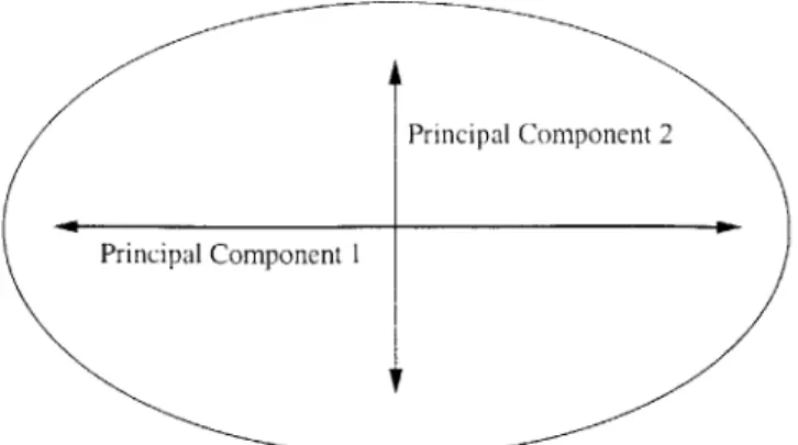
4-1 Principal components of an ellipse are the primary and secondary axis 55 4-2 Functional Class Histogram . . . . 60

5-1 A maximal margin hyperplane that correctly classifies all points on either half-space [191 . . . . 65

List of Tables

2.1 Tissue D ata Sets . . . . 29

3.1 Linear Separability of the Tissue Data . . . . 43

4.1 Genes Selected by Mean Difference Technique . . . . 61

5.1 Jack-knifing Error Percentages... ... 80

Chapter 1

Introduction

1.1

Motivation

Oligonucleotide array technology has recently been developed, which allows the mea-surement of expression levels of thousands of genes simultaneously. This technology provides biologists with an opportunity to view the cell at a systems level instead of one subsystem at a time in terms of gene expression. Clearly, this technology is suited for study of diseases that have responses at the transcriptional level.

One such disease is cancer. Many studies have been done using oligonucleotide arrays to gather information about how cancer expresses itself in the genome. In the process of using these arrays, massive amounts of data have been produced.

This data has, however, proven difficult for individuals to just "look" at and extract significant new insights due to its noisy and high dimensional nature. Com-putational techniques are much better suited, and hence are required to make proper use of the data obtained using oligonucleotide arrays.

1.1.1 Cancer Mortality

Cancer is the second leading cause of death. Nearly 553,000 people are expected to (lie of cancer in the year 2001 [21]. Efforts on various fronts utilizing array technology are currently underway to increase our understanding of cancer's mechanism.

One effort is focused on identifying all genes that are related to the manifestation of cancer. While a few critical genes have been identified and researched (such as

p53, Ras, or c-Myc), many studies indicate that there are many more genes that are

related to the varied expression of cancer. Cancer has been shown to be a highly differentiated disease, occurring in different organs, varying in the rate of metastasis, as well as varying in the histology of damaged tissue. It has been hypothesized that different sets of "misbehaving" genes may be causing these variances, but as of yet these genes have not yet been identified for many of the different forms of cancer. Identifying these various genes could aid us in understanding the mechanism of cancer, and potentially lead to new treatments. Monitoring the expression of several thousands of genes using oligonucleotide arrays has increased the probability of finding cancer causing genes.

Another effort has focused on utilizing oligonucleotide arrays as diagnosis tools for cancer. Given our current methods of treatment, it has been found that the most effective way of treating cancer is to diagnose its presence as early as possible and as specifically as possible. Specific treatments have been shown to perform significantly better on some patients compared to others, and hence the better we are able to identify the specific type of cancer a patient has, the better we are able to treat that patient. A diagnosis tool that can accurately and quickly determine the existence and type of cancer would clearly be beneficial. Again, because cancer has been shown to be a genetic disease, many efforts have been made to provide a cancer diagnosis tool that measures the expression of genes in cells. Since such technologies have been recently developed, most of the focus has been on finding a set of genes which accurately determine the existence of cancer.

The goal of this thesis is to aid in both of the efforts mentioned above, namely to discover "new" genes that are causes of various types of cancers, and using these genes provide an accurate cancer diagnosis tool.

1.1.2

Usage and Availability of Genechip Data

The usage of oligonucleotide arrays is not limited to the study of cancer. Oligonu-cleotide arrays have been used to study the cell cycle progression in yeast, specific cellular pathways such as glycolysis, etc. In each case, however, the amount of data is large, highly dimensional, and typically noisy. Computational techniques that can extract significant information are extremely important in realizing the potential of the array technology.

Therefore, an additional goal of this thesis was to contribute a new process of array analysis, using a combination of computational learning techniques to extract significant information present in the oligonucleotide array data.

1.2

Related Array Analysis

Because cancer is primarily a genetic disease (See Ch 2.1), there have been numer-ous studies of varinumer-ous types of cancer using oligonucleotide arrays to identify can-cer related genes. The typical study focuses on one organ-specific cancan-cer, such as prostate cancer. First, tissue samples from cancerous prostates (those with tumors) and healthy prostates are obtained. The mRNA expression levels of the cells in each of the samples is then measured, using an oligonucleotide array per sample. The resulting data set can be compactly described as an expression matrix V, where each column represents the expression vector C of an experiment, and each row represents the expression vector ' of a gene. Each element Vj is a relative mRNA expression level of the 7'h gene in the Jth sample.

UVii V₁₂ - - - Vn

- V_{2 1} V22 . .. V2 n

\

0

n1 Vn2 . . Vnmn

The study then introduces a new computational technique to analyze the data gathered. The ability of the technique to extract information is first validated, by analyzing a known data set and/or by comparing the results obtained through other traditional techniques. Typically, the new technique is then used to make new asser-tions, which may be cause for future study. All of the techniques can be classified in two categories: unsupervised and supervised learning techniques. A description of the techniques applied to array data follows.

Unsupervised learning techniques focus on finding structure in the data, while supervised learning techniques focus on making classifications. The main difference between unsupervised and supervised learning techniques is that supervised learning techniques use user-supplied information about what class an object belongs to, while unsupervised techniques do not.

1.2.1

Unsupervised Learning Techniques

Unsupervised learning techniques focus on discovering structure on the data. The word "discover" is used because unlike supervised learning techniques, unsupervised techniques have no prior knowledge (nor any notion) about what class a sample belongs to. Most of the techniques find structure in the data based on similarity measures.

Clustering

One major class of unsupervised learning techniques is known as clustering. Clus-tering is equivalent to grouping similar objects based on some similarity measure.

A similarity function

f(Y,

z) is typically called repeatedly in order to achieve the

final grouping. In the context of arrays, clustering has been used to group similar experiments and to group similar genes. Researchers have been able to observe the expression of cellular processes across different experiments by observing the expres-sion of sets of genes obtained from clustering, and furthermore associate functions for genes that were previously unannotated. By clustering experiments, researchers

have, for example, been able to identify new subtypes ofcancers. Three algorithms that have been utilized to do clustering on genomic data are hierarchical clustering, k-means clustering, and Self Organizing Maps (SOMs).

Hierarchical clustering was first applied to oligonucleotide array data by Eisen

et al. [6]. The general algorithm uses a similarity metric to determine the highest

correlated pair of objects among the set of objects to be clustered C. This pair is then

clustered together, removed from the set C, and the average of the pair is added to

C. The next iteration proceeds similarly, with the highest correlated pair in C being

removed and being replaced by a single object. This process continues until C has only

one element. The clustering of pairs of objects can be likened to leaves of a tree being joined at a branch, and hence a dendrogram can be used to represent the correlations between each object. Eisen et al. used several similarity measures and tried different remove/replace policies for the algorithm. They were able to demonstrate the ability of this technique by successfully grouping genes of known similar function for yeast. Specifically, by clustering on 2,467 genes using a set of 12 time-course experiments that measured genomic activity throughout the yeast cell cycle, several clusters of genes corresponding to a common cellular function were found. One cluster was comprised of genes encoding ribosomal proteins. Other clusters found contained genes involved in cholesterol biosynthesis, signaling and angiogenesis, and tissue remodeling and wound healing.

K-means clustering is a technique that requires the user to input the number of expected clusters, and often, the coordinates of the centroids in n dimensional space (where n corresponds to the number of variables used to represent each object). Once this is done, all points are assigned to their closest centroid (based on some similarity metric, not necessarily euclidean distance), and the centroid is recomputed

by averaging the positions of all the points assigned to it. This process is repeated

until each centroid does not move after recomputing its position. This technique effectively groups objects together in the desired number of bins.

Self Organizing Maps (SOMs) is another clustering technique that is quite similar to k-means [23]. This technique requires al input: the geometry in which the number

of expected clusters in the data is expected. For example, a 3x2 grid means that a total of six clusters are expected in the data. This grid is then used to calculate the positions of six centroids in n dimensional space. The SOM algorithm then randomly selects a data point and moves the closest centroid towards that point. As the distance between each successive (randomly selected) data point and the closest centroid decreases, the distance the centroid moves decreases. After all points have been used to move the centroids, the algorithm is complete. This technique was used to cluster genes and identify groups of genes that behaved similarly for yeast cell cycle array data. SOMs were able to find clusters of yeast genes that were active in the respective G1,S, G2, and M phases of the cell cycle when analyzing 828 genes over 16 experiments using a 6x5 grid. While the obtained clusters were desirable, the selection of the grid was somewhat arbitrary and the algorithm was run until results matching previous knowledge were obtained.

As noted above, clustering can be performed by either clustering on genes or clustering on experiments. When both clusterings are performed and the expression matrix is rearranged accordingly, this is known as two-way clustering. Such an anal-ysis was done on cancerous and non-cancerous colon tissue samples [1]. The study conducted by Alon et al. was the first to cluster on genes (based on expression across experiments) and cluster on experiments (based on expression across genes). Given a data set of 40 cancererous and 22 normal colon tissue samples on arrays with 6500 features, the clustering algorithm used was effective at grouping the cancer and nor-mal tissues respectively. Alon et al. also attempted to use a method similar to that described in Ch 4.1.1 to reduce the data set and observe the resulting classification performance of the clustering algorithm.

Dimension Reduction

Dimension reduction is a type of technique that reduces the representation of data by finding a few components that are repeatedly expressed in the data. Linear dimension reduction techniques use linear combinations of these components to reconstruct the original data. Besides finding a space saving minimal representation, such techniques

are useful because by finding the critical components, they essentially group together dimensions that behave consistently throughout the data.

Given V as the original data, dimension reduction techniques perform the

follow-ing operation: V ~ W * H. The critical components are the columns of the matrix

W. Given an expression matrix V, each column of W can be referred to as a "basis array". Each basis array contains groupings of genes that behave consistently across each of the arrays. Just as before, since the genes are all commonly expressed in the various arrays, it is possible that they are functionally related. If a basis array is rela-tively sparse, it can then be interpreted to represent a single cellular processes. Since an experiment is a linear combination of such basis arrays, it can then be observed which cellular processes are active in an experiemnt.

There are several types of linear dimension reduction techniques, all using the notion of finding a set of basis vectors that can be used to reconstruct the data. The techniques differ by placing different constraints to find different sets of basis vectors. For more details, please see Ch 4.2.

The most common technique used is Principal Components Analysis (PCA). PCA decomposes a matrix into the critical components as described above (known as eigen-vectors), but provides an ordering of these components. The first vector (principal component) is in the direction of the most variability in the data, and each successive component accounts for as much of the remaining variability in the data as possible. Alter et al. applied PCA to the expression matrix, and were able to find a set of principal components where each component represented a group of genes that

were active during different stages of the yeast cell cycle [2]. Fourteen time-course

experiments were conducted over the length of the yeast cell cycle using arrays with 6,108 features. Further study of two principal components were able to effectively represent most of the cell cycle expression oscillations.

Another method known as Non-negative Matrix Factorization (NMF) has been used to decompose oligonucleotide array into similarly interesting components that represent cellular processes (Kim & Tidor, to be published). NMF places the con-straint that each basis vector has only positive values. PCA, in contrast, allows for

negative numbers in the eigenvectors. NMF leads to a decomposition that is well suited for oligonucleotide array analysis. The interaction between the various basis vectors is clear: it is always additive. With PCA, some genes may be down-regulated in a certain eigenvector while they maybe be up-regulated in another. Combining two eigenvectors can cancel out the expression of certain cellular processes, while com-bining two basis vectors from NMF always results in the expression of two cellular processes. In this sense, NMF seems to do a slightly better job selecting basis vectors that represent cellular processes.

Other methods of dimensionality reduction exist as well, such as Multidimensional Scaling (MDS) and Locally Linear Embedding (LLE, a type of non-linear dimen-sionality reduction) [10, 20]. Both of these techniques are more commonly used as visualization techniques. See Ch 3.1 and 3.2 for more details.

1.2.2

Supervised Learning Techniques

Supervised learning techniques take advantage of user provided information about what class a set of objects belong to in order to learn which features are critical to the differentiation between classes, and often to come up with a decision function that distinguishes between classes. The user provided information is known as the training set. A "good" (generalizable) decision function is then able to accurately classify samples not in the training set.

One technique that focuses on doing feature selection is the class predictor method-ology developed by Golub et al.

[9]

that finds arbitrarily sized sets of genes that could be used for classification. The technique focuses on finding genes that have an ideal-ized expression pattern across all arrays, specifically genes that have high expression among the cancerous arrays and low expression among the non-cancerous arrays. These genes are then assigned a predictive power, and collectively are used to decide whether an unknown sample is either cancerous or non-cancerous (refer to Ch 4.2 for more details of the algorithm). Golub et al. were able to use the above technique to distinguish between two types of leukemias, discover a new subtype of leukemia, and to determine the class of new leukemia cases.

One technique that seeks to solve the binary classification problem (classification into two groups) is the Support Vector Machine (SVM). The binary classification problem can be described as finding a decision surface (or separating hyperplane)

in iL dimensions that accurately allows all samples of the same class to be in the

same half-space. The Golub technique is an example of a linear supervised learning method, because the decision surface described by the decision function is "flat". In contrast, non-linear techniques create decision functions with higher-order terms that correspond to hyperplanes which have contours. SVMs have the ability to find such non-linear decision functions.

Several researchers have utilized SVMs to obtain good classification accuracy using oligonucleotide arrays to assign samples as cancerous or non-cancerous [4, 8, 17]. This computational technique classifies data into two groups by finding the "maximal margin" hyperplane. In a high dimensional space with a few points, there are many hyperplanes that can be used to distinguish two classes. SVMs choose the "optimal" hyperplane by selecting the one that provides the largest separation between the two groups. In the case where a linear hyperplane can not be found to separate the two groups, SVMs can be used to find a non-linear hyperplane by projecting the data into a higher dimensional space, finding a linear hyperplane in this space, and then projecting the linear hyperplane into the original space which causes it to be non-linear. See Ch 5 for more details.

1.3

Approach to Identifying Critical Genes

In order to extract information from the data produced by using oligoiucleotide arrays, computational techniques which are able to handle large, noisy, and high dimensional data are necessary. Since our goal is two-tiered:

" to discover new genes critical to cancer

" to create a diagnosis tool based on measurements of expression of a small set of

our proposed solution is two-tiered as well:

" use various feature selection techniques to discover these cancer causing genes " use a supervised learning technique to create a decision function that can serve

as a diagnosis tool, as well as to validate and further highlight cancer-related genes

One of several feature selection methods will be used to reduce the dimensionality of a cancer data set. The dimensionally reduced data set will then be used as a training set for a support vector machine, which will build a decision function that will be able to classify tissue samples as "cancerous" or "normal". The success of the feature selection method can be tested by observing the jack-knifing classification performance of the resulting decision function. Also, the decision function can be further analyzed to determine which variables are associated the heaviest "weight" in the decision function, and hence are the most critical differentiators between cancerous and non-cancerous samples.

Pre-Processing

Visualization

Feature Space Reduction

Support Vector Classification

The feature selection method will not only find critical cancer-causing genes, but will reduce the dimensionality of the data set. This is critical because it has been

shown that when the number of features is much greater than the number of

sam-ples, the generalization performance of the resulting decision function suffers. The feature selection method will be used to improve the generalizability of the decision function, while the generalization performance of the SVM can also be used to rank the effectiveness of each feature selection method.

Besides providing a potential diagnosis tool, analysis of a highly generalizable decision function found by SVMs may also highlight critical genes, which may war-rant future study. SVMs were the chosen supervised learning method due to their ability to deterministically select the optimal decision function, based on maximizing the margin between the two classes. The maximal margin criteria has been proven to have better (or equivalent) generalization performance when compared to other supervised learning methods, such as neural nets, while the decision function's form (linear, quadratic, etc.) can be easily and arbitrarily selected when using SVMs. This increases our ability to effectively analyze and use the resulting decision function as a second method of feature selection.

Chapter 2

Background

The first section of this chapter will describe the basic mechanisms of cancer, as well as demonstrate the applicability of oligonucleotide arrays to the study of cancer. The second section discusses how the array technology works, its capabilities, and its limitations. Our specific datasets will be described, and then the various techniques commonly used to prepare array data will also be presented.

2.1

Basic Cancer Biology

Cancer is Primarily a Genetic Disease

Cancer is caused by the occurrence of a mutation that causes the controls or regulatory elements of a cell to misbehave such that cells grow and divide in an unregulated fashion, without regard to the body's need for more cells of that type.

The macroscopic expression of cancer is the tumor. There are two general cate-gories of tumors: benign, and malignant. Benign tumors are those that are localized and of small size. Malignant tumors, in contrast, typically spread to other tissues. The spreading of tumors is called metastasis.

There are two classes of gencs that have been identified to cause cancer: oncogenes, and tunior-suppressor genes. An oncogene is defined as any gene that encodes a protein capable of' transforming cells in culture or inducing cancer in animals. A

tumor-suppressor gene is defined as any gene that typically prevents cancer, but when mutated is unable to do so because the encoded protein has lost its functionality.

Development of cancer has been shown to require several mutations, and hence older individuals are more likely to have cancer because of the increased time it typically takes to accumulate multiple mutations.

Oncogenes

There are three typical ways in which oncogenes arise and operate. Such mutations result in a gain of function [15]:

" Point mutations in an oncogene that result in a constitutively acting (constantly

"on" or produced) protein product

" _{Localized gene amplification of a DNA segment that includes an oncogene,} leading to over-expression of the encoded protein

" Chromosomal translocation that brings a growth-regulatory gene under the

con-trol of a different promotor and that causes inappropriate expression of the gene

Tumor-Suppressor Genes

There are five broad classes of proteins that are encoded by tumor-suppressor genes. In these cases, mutations of such genes and resulting proteins cause a loss of function

[15]:

* Intracellular proteins that regulate or inhibit progression through a specific stage of the cell cycle

* Receptors for secreted hormones that function to inhibit cell proliferation * Checkpoint-control proteins that arrest the cell cycle if DNA is damaged or

chromosomes are abnormal

* Proteins that promote apoptosis (programmed cell death) " Enzymes that participate in DNA repair

2.2

Oligonucleotide Arrays

The oligonucleotide array is a technology for measuring relative mRNA expression levels of several thousand genes simultaneously [14]. The largest benefit of this is that all the gene measurements can be done under the same experimental conditions, and therefore can be used to look at how the whole genome as a system responds to different conditions.

The 180 oligonucleotide arrays that compose the data set which I am analyzing were commercially produced by Affymetrix, Inc.

Technology

GeneChips, Affymetrix's proprietary name for oligonucleotide arrays, can be used to determine relative levels of mRNA concentrations in a sample by hybridizing complete cellular mRNA populations to the oligonucleotide array.

The general strategy of oligonucleotide arrays is that for each gene whose expres-sion is to be measured (quantified by its mRNA concentration in the cell), there are small segments of nucleotides anchored to a piece of glass using photolithography techniques (borrowed from the semiconductor industry, hence the name GeneChips). These small segments of nucleotides are supposed to be complementary to parts of the gene's coding region, and are known as oligonucleotide probes. In a certain area on the piece of glass (specifically, a small square known as a feature), there exist hun-dreds of thousands of the exact same oligonucleotide probe. So, when a cell's mRNA is washed over the array using a special procedure with the correct conditions, the segments of mRNA that are complementary to those on the array will actually hy-bridize or bind to one of the thousands of probes. Since the probes on the array are designed to be complementary to the mRNA sequence of a specific gene, the overall amount of target mRNA (from the cell) left on the array gives an indication of the mRNA cellular concentration of such a gene.

In order to actually detect the amount of target mRNA hybridized to a feature on the array, the target mRNA is prepared with fluorescent material. Since all the probes

for a specific gene are localized to a feature, the amount of fluorescence emitted from the feature can be measured and then interpreted as the level of hybridized target mRNA.

Genechips

Affymetrix has developed their oligonucleotide arrays with several safeguards to im-prove accuracy. Because there may be other mRNA segments that have comple-mentary nucleotide sequences to a portion of a probe, Affymetrix has included a "mismatch" probe which has a single nucleotide inserted in the middle of the original nucleotide sequence. The target mRNA (for the desired gene) should not bind to this mismatch probe. Hence, the amount of binding mRNA to the mismatch probe is supposed to represent some of the noise that also binds to portions of the match probe. By subtracting the amount of mRNA hybridized to the mismatch probe from the amount of mRNA hybridized to the match probe, a more accurate description of the amount of the target gene's mRNA should be obtained.

Since the oligonucleotide probes are only approximately 25 nucleotides in length and the target gene's mRNA is typically 1000 nucleotides in length, Affymetrix selects multiple probes that hybridize the best to the target mRNA while hybridizing poorly to other mRNA's in the cell. The nucleotide sequences for the probes are not released

by Affymetrix. Overall, to measure the relative mRNA concentration of a single gene,

approximately 20 probe pairs (20 match probes and 20 mismatch probes) exist on the chip.

A measure provided by Affymetrix uses the 20 probe pairs and computes an overall

expression value for the corresponding gene is known as the "average difference". Most techniques utilize the average difference value instead of analyzing the individual intensity values observed at each of the 40 probes. The measure is calculated as

follows

average difference =

n

vector, and mrA is the mismatch probe set expression vector.

Capabilities

A major benefit of oligonucleotide arrays is that they provide a snapshot view of nearly

an entire system by maintaining the same set of experimental conditions for each measurement of each gene. This lends itself to analysis of how different components interact among each other. Another important benefit is that the use of the arrays produces a large amount of data quickly. Previously, experiments to measure relative mRNA expression levels would go a few at time. Using the arrays, thousands of measurements are quickly produced. From an experimental point of view, another benefit of using oligonucleotide arrays is that the method requires less tedious steps such as preparing clones, PCR produces, or cDNAs.

Limitations

There are several problems with the usage of oligonucleotide arrays. Some issues related to the oligonucleotide technology are:

" the manner in which expression levels are measured lacks precision (via

fluo-rescence), because genes with longer mRNA will have more fluorescent dyes attached than those genes with shorter mRNA, resulting in higher fluorescence for genes with longer mRNA

* absolute expression levels cannot be interpreted from the data

" no standards for gathering samples for gene chips, and hence conditions in which

the experiments are done are not controlled

" probes used may not accurately represent a gene, or may pick up too much

noise (hybridization to mRNA of genes other than the target gene) resulting in negative average difference values

Another issue related to using oligonucleotide arrays is that some important or critical genes may not be on the standard genechips, made by Affymetrix. A more

general issue is that while mRNA concentrations are somewhat correlated to the asso-ciated protein concentrations, it is not understood to what degree they are correlated. Also, some proteins are regulated at the transcription level, while some are regulated at the translation level. Ideally, there would be arrays that measured protein concen-trations of all the proteins in the organism to be studied. Analyzing relative amounts of mRNA (at the transcription level) is basically one step removed from such desired analysis.

2.3

Data Set Preparation

Two sets of oligonucleotide array data have been provided for analysis by John B. Welsh from the Novartis Foundation. Both sets use Affymetrix genechips, but each set has used a different version of the cancer genechip, which contains genes that are

(in the judgment of Affymetrix) relevant to cancer and its cellular mechanisms. The first data set uses the HuGeneFL genechip from Affymetrix, which contains probes with length of 25 nucleotides. These chips contain over 6000 probe sets, with 20 (perfect match, mismatch) probe pairs per probe set. Each probe set corresponds to a gene. The data set is composed of 49 such arrays, with 27 arrays used to measure the expression patterns of cancerous ovarian tissue, and 4 arrays used to measure the expression patterns of normal ovarian tissue. The rest of the arrays were used to test the expression patterns of cancer cell lines, as well as to perform duplicate experiments. The method of preparation of these experiments was published by Welsh et al. [25]. 1

The second data set uses the U95avl and U95av2 genechip from Affymetrix. The two versions each contain probe sets for over 12,000 genes. Each probe set contains

16 probe pairs of probes of length 25. The two chips differ only by 25 probe sets,

and hence by using only the common sets, the experiments can be treated as being from one type of genechip. This data set is composed of 180 genechip experiments,

'While the HuGeneFL genechips were used for initial analysis, all the analysis included in this thesis is performed on the second data set.

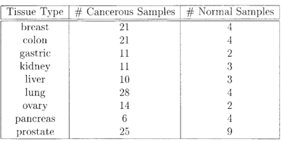
Table 2.1. Tissue Data Sets

Tissue Type

#

Cancerous Samples

#

Normal Samples

breast 21 4 colon 21 4 gastric 11 2 kidney 11 3 liver 10 3 lung 28 4 ovary 14 2 pancreas 6 4 prostate 25 9

from 10 different cancer tissues. There are approximately 35 normal tissue samples, and 135 cancerous tissue samples. The various tissues include breast, colon, gastric, kidney, liver, lung, ovary, pancreas, and prostate.

It is important to note that the number of cancerous samples is in almost all cases, much larger than the number of normal samples. Ideally, these numbers would be equal to each other. Also, the tissue data sets themselves are not particularly large. They might not be able to provide a generalizable diagnostic tool because of the limited size of the training set. One last issue is that the "normal" tissue samples are not from individuals who are without cancer. Tissue samples are "normal" if they do not exhibit any metastasis or tumors. Often the normal samples are taken from individuals with a different type of cancer, or just healthy parts of the tissue that contains tumors.

2.4

Data Preprocessing Techniques

Various preprocessing techniques can affect the ability of an analysis technique sig-nificantly. Using genechips, there are three common ways of preprocessing the data that have been used in the analysis of the above data sets. Additionally, there are some preprocessing techniques which were used to remove poor quality data.

Removal of "Negative" Genes

The first major concern regarding the quality of the data sets above is that there are large numbers of genes with negative average difference values. Clearly, negative expression of a gene has no meaning. Negative average difference values mean that among all probe pairs in a probe set, there is more binding to the mismatch probe than there is to the match probe on average. Ideally, the probes would have been selected such that this would not happen. The exact biological explanation for such behavior is not known, and hence it is unclear whether to interpret the target gene as present or not since the same nonspecific mRNAs that hybridized to the mismatch probe could be hybridized to the respective perfect match probe as well, causing the perfect match probe to have a high fluorescent intensity.

One approach is to remove any genes which have any negative average difference values from consideration. Hence, when comparing arrays using computational tech-niques, any gene which has had a negative average difference value in any array will be removed and hence that dimension or variable will not be used by the technique to differentiate between arrays.

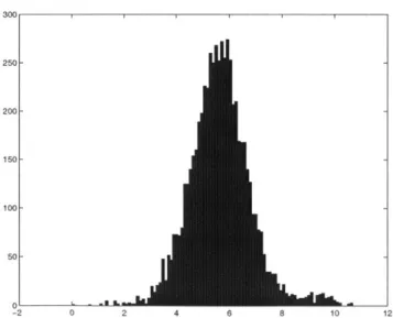
Log Normalization

The log function has the interesting property that given a distribution, it has the abil-ity to make it appear more gaussian. Gaussian distributions have statistical properties such that the statistical significance of a result can be established.

As can be seen from the figures above, log normalizing the data has the effect of compressing the data close to the intervals, while stretching out the data in the middle of the original distribution. One issue is that the log of a negative number is not defined, which is another reason to remove genes with negative average difference values.

40UU I I I I 4000 3500 3000 2500 2000 1500 1000 500 0 0 0.5 1 1.5 2 2.5 3 3.5 4 4.5 x 10" Figure 2-1. Histogram of unnormalized gene expression for one array

250- 200- 150- 100-50 0L ' - " -2 0 2 4 6 8 10 12

Global Scaling

When making preparations for a genechip experiment, many variables can affect the amount of mRNA which hybridizes to the array. If differences in the preparation exist, they should have a uniform effect on the data such that one experiment's average difference values for all genes would be, for example, consistently higher than those for another experiment's. When doing analysis on the arrays, it is desirable to eliminate these effects so the analysis can be focused on "real" variations in the cell's behavior, not differences in the preparation of the experiment.

One common way to do this is to scale each array such that the means of the average difference values are equal to each other, some arbitrary number c. This is illustrated below for an array with expression vector Y with n average difference values:

C * X* _{( n}

-n

This effectively removes the effects of variation in the preparation of the experiments.

Mean-Variance Normalization

Another technique used to transform the data and remove the effects of the prepara-tion of the experiment is to mean-variance normalize the data. In order to do this, the mean pu and standard deviation o- for each array Y is calculated. Each average difference value xi is transformed:

xi - px

The resulting number represents the number of standard deviations the value is from the mean (commonly known as a z-score). An important result of this type of nor-malization is that it also removes the effects of scaling.

Chapter 3

Visualization

To better understand the information content in the oligonucleotide array data sets, the first goal was to attempt to visualize the data. Since many computational tech-niques focus on grouping the data into subgroups, it would be useful to see 1) how well the traditional grouping techniques such as hierarchical/k-means clustering perform 2) how the data looks projected into dimensions that can be visualized by humans easily (specifically, three dimensions). By visualizing the data, we can understand how much noise (relative to the information) is in the data, possibly find inconsisten-cies in the data, and predict which types of techniques might be useful in extracting information from the data.

Visualization techniques also enable us to understand how various transformations on the data affect the information content. Specifically, in order to understand how each preprocessing technique (described in Ch 2.4) affects the data, we can apply the preprocessing technique to the data, and observe the effect by comparing the original data visualization versus the modified data visualization.

3.1

Hierarchical Clustering

Technique Description

Hierarchical clustering is an unsupervised learning technique that creates a tree which shows the similarity between objects. Sub-trees of the original tree can be seen as a group of related objects, and hence the tree structure can indicate a group-ing/clustering of the objects.

Nodes of the tree represent subsets of the input set of objects S. Specifically, the set S is the root of the tree, the leaves are the individual elements of S, and the internal nodes represent the union of the children. Hence, a path down a well constructed tree should visit increasingly tightly-related elements [7]. The general algorithm is included below:

" calculate similarity matrix A using set of objects to be clustered

" while number of columns/rows of A is > 1

1. find the largest element Aj

2. replace objects i and

j

by their average in the set of objects to be clustered 3. recalculate similarity matrix A with new set of objects

Variations on the hierarchical clustering algorithm typically stem from which sim-ilarity coefficient is used, as well as how the objects are joined. Euclidean distance, or the standard correlation coefficient are commonly used as the similarity measure. Objects or subsets of objects can be joined by averaging all their vectors, or averaging two vectors from each subset which have the smallest distance between them.

Expected Results on Data Set

Ideally, using the hierarchical clustering technique we would obtain two general clus-ters. One cluster would contain all the cancer samples, and another cluster would contain all the normal sample. Since the hypothesis is that cancer samples should have roughly similar expression pattern across all the genes, all these samples should be

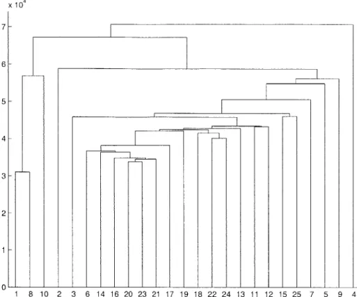
x 104 7- 6- 5- 4- 3- 21 - 0-1 8 10 2 3 6 14 16 20 23 21 17 19 18 22 24 13 11 12 15 25 7 5 9 4

Figure 3-1. Experiments 1, 2, 8, and 10 are normal breast tissues. Hierarchical clustering performed using euclidean distance and most similar pair replacement policy

grouped together. Similarly, normal samples should be grouped together. Although using the hierarchical clustering algorithm the sets of cancer and normal samples will be joined at a node of the tree, ideally the root of the tree would have two children, representing the cancer and normal sample clusters. This would show that the dif-ference between cancer and normal samples is on average larger than the variation inside each subset.

Results

Four different variations of hierarchical clustering were performed on 4 expression matrices per tissue. The 4 variations of clustering resulting from utilizing 2 different similarity metrics (euclidean distance, and pearson coefficient) with 2 remove/replace policies (removing the most similar pair and replacing with the average, removing the most similar pair and replacing with the sample that was most similar to the remaining samples).

For each tissue, the original expression matrix (after removing negative genes, see

Ch 2.4) was clustered on as well as three other pre-processed expression matrices.

Log normalization, mean-variance normalization, and global scaling were all applied and the resulting expression matrices were clustered.

For most of the tissues, across all the different variations of clustering and the differently processed data sets, the desired results were obtained. The normal samples were consistently grouped together, forming a branch of the resulting dendrogram. However, the set of cancer samples and set of normal samples were never separate branches that joined at the root. This would have indicated that for each sample in each set, the most dissimilar object within the set was still more similar than a sample from the other set. Apparently, the amount of separation between the sets of cancer and normal samples is not large enough to give this result.

3.2

Multidimensional Scaling (MDS)

Technique Description

Each multidimensional object can be represented by a point in euclidean space. Given several objects, it is often desirable to see how the objects are positioned in this space relative to each other. However, visualization beyond 3 dimensions is typically non-intuitive. Multidimensional scaling (MDS) is a technique that can project multidi-mensional data into an arbitrary lower dimension. The technique is often used for visualizing the relative positions of multidimensional objects in 2 or 3 dimensions.

The MDS method is based on dissimilarities between objects. The goal of MDS is to create a picture in the desired n dimensional space that accurately reflects the dissimilarities between all the objects being considered. Objects that are similar are shown to be in close proximity, while objects that are dissimilar are shown to be distant. When dissimilarities are based on quantitative measures, such as euclidean distance or the correlation coefficient, the MDS technique used is known as metric

" use euclidean distance to create a dissimilarity matrix D

" scale the above matrix: A = -0.5 * D2

* center A : a = A-(row means of A)-(column means of A)-+(mean of all elements of A) " obtain the first n eigenvectors and the respective eigenvalues of a

" scale the eigenvectors such that their lengths are equal to the square root of their respective eigenvalues

" if eigenvectors are columns, then points/objects are the rows, and plot

Typically, euclidean distance is used as the dissimilarity measure. MDS selects n dimensions that best represent the differences between the data. These dimensions are the eigenvectors of the scaled and centered dissimilarity matrix with the n largest eigenvalues.

Expected Results on Data Set

By looking at the 3-dimensional plot produced by MDS, the most important result to observe is that cancer samples group together and are separable in some form from the normal samples. Given that the two sets do separate from each other in 3 dimensions, the next step would be to see what type of shape is required to separate the data. It would be helpful to note whether the cancer and normal samples were linearly separable in 3 dimensions, or required some type of non-linear (e.g. quadratic) function for separation. The form of this discriminating function would then be useful when choosing the type of kernel to be used in the support vector machine (Ch 5.1).

Results

MDS was used to project all nine tissue expression matrices into 3 dimensions. For each tissue, the original data (without any negative genes, see Ch 2.4) was used to create one plot. To explore the utility of the other pre-processing techniques described in Ch 2.4, three additional plots were made. Log normalization, mean-variance normalization, and global scaling were all applied to the expression matrices

MDS into 3 Dimensions of 25 breast samples x cancerous sample 0 non-cancerous sample 20, 15, 0 0 10, 5, X 0 X -5 X X -10 * -15, X -20 x x -25 30 20 10 40 0 20 -10 0 -20 -20 -30 -40

Figure 3-2. Well clustered data with large separation using log normalized breast tissue data set

(without negative genes), and then the resulting expression matrices were projected into 3 dimensions.

The first observation is that in most of the 3-D plots, the cancer samples and normal samples group well together. In some cases, however, the separation of the two sets can not be clearly seen. The linear separability of such tissues will be determined when SVMs are used to create decision functions with a linear kernel (see

Ch. 5.3). Please refer to Ch 3.4 for a summary of which tissues are linearly separable,

and the apparent margin/separation between the cancer and normal samples.

Another general observation is that log transforming the data seems to improve in separating the data sets the best among the pre-processing techniques, although mean-variance normalization also often increases the margin of separation.

3.3

Locally Linear Embedding (LLE)

Technique Description

Like MDS and hierarchical clustering, locally linear embedding (LLE) is a unsuper-vised learning algorithm, i.e. does not require any training to find structure in the

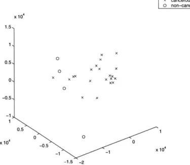
MDS into 3 Dimensions of 25 colon samples cancerous sample OX non-cancerous sample x 104 1.5, 0x X 0.5, OX 0 X X X o, xx _)O x 0 -0.5, x x -1 0.5 0 0 x 104 -0.5 ₀ -1 -1 10 -1.5 -2

Figure 3-3. Poorly separated data, but the two sets of samples are reasonably clustered.

data [20]. Unlike these two techniques, LLE is able to handle complex non-linear rela-tionships among the data in high dimensions and map the data into lower dimensions that preserve the neighborhood relationships among the data.

For example, assume you have data that appears to be on some type of nonlinear manifold in a high dimension like an S curve manifold. Most linear techniques that project the data to lower dimensions would not recognize that the simplest represen-tation of the S curve is just a flat manifold (the S curve stretched out). LLE however is able to recognize this, and when projecting the higher dimensional data to a lower dimension, selects the flat plane representation.

This is useful because LLE is able to discover the underlying structure of the manifold. A linear technique such as MDS would instead show data points that are close in euclidean distance but distant in terms of location on the manifold, as close in the lower dimension projection. Specifically relating to the cancer and normal oligonucleotide samples, if the cancer samples were arranged in some high dimensional space on a non-linear manifold, LLE would be able to project the data into a lower dimensional space while still preserving the locality relationships from the higher dimensions. This could provide a more accurate description of how the cancer and

4 + + +4: + +* + ++ t4 + A 1 * + +**4. + ++ 444

Figure 3-4. LLE trained to recognize S-curve [20]

normal samples cluster together.

The basic premise of LLE is that on a non-linear manifold, a small portion of the manifold can be assumed to be locally linear. Points in these locally linear patches can be reconstructed by the linear combination of its neighbors which are assumed to be in the same locally linear patch. The coefficients used in the linear combination can then be used to reconstruct the points in the lower dimensions. The algorithm is included below:

* for each point, select K neighbors

+2

* minimize the error function E(W) = >ji Xi -

Z

₃ Wi~ , where the weights

Wig represent the contribution of the jth data point to the ith reconstruction,

with the following two constraints:

1. W7i, is zero for all Xy that are not neighbors of Xi

2. EZ Wi = 1

* map Xi from dimension D to Yi of a much smaller dimension d using the

Wij's obtained from above by minimizing the embedding cost function <D(Y) =

2

The single input to the LLE algorithm is K, the number of neighbors used to re-construct a point. It is important to note that in order for this method to work, the manifold needs to be highly sampled so that a point's neighbors can be used to reconstruct the point through linear combination.

Expected Results on Data Set

If the normal and cancer samples were arranged on some type of high dimensional

non-linear manifold, it would be expected that the visualization produced by LLE would show a more accurate clustering of the samples to the separate sets. However, since there are relatively few data points, the visualization might not accurately represent the data.

Results

LLE was performed in a similar fashion as MDS on the nine tissues, with four plots

produced for each tissue corresponding to the original expression matrix, log normal-ized matrix, mean-variance normalnormal-ized matrix, and globally scaled matrix (where all matrices have all negative genes removed).

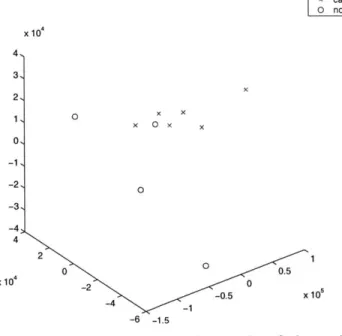
LLE in general produces 3-d projections quite similar to those produced by MDS.

However, one notable difference is the tendency of LLE to pull samples together. This effect is also more noticable as the number of samples is large. This is clearly an artifact of the neighbor-based nature of algorithm.

The LLE plots reinforce the statements regarding the abilities of the pre-processing techniques to increase the separation between the cancer and normal samples. While log normalizing the data produces good separation, inean-variance normalizating seems to work slightly better. Nonetheless, both log normalization and mean-variance normalization both seem to be valuable pre-processing techniques according to both projection techniques.

LLE (w/5 nearest neighbors) into 3-D of 32 lung samples x cancerous sample 0 non-cancerous sample 2, 1, 0. -11 -2. 3 xX xx 0 0 0 0 x 0 3i x 2 X x 2 1 0 0 -2 -1-4

Figure 3-5. Branching of data in LLE projection

MDS into 3 Dimensions of 32 lung samples

cancerous sample 0 non-cancerous sample x 104 5, 4., 3,. 2, 1 . -11 -2, -3 1 x x x XX X X x X xx x x x x x 0 0 0 4 0 2 15 0 x104 -2 10 -4 5 X 104 -6 0 -8 -5

Figure 3-6. MDS projections maintain relative distance information x

x x x x

3.4

Information Content of the Data

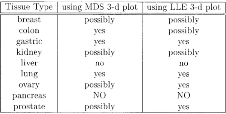
After observing each of the plots produced by both LLE and MDS, we are able to draw some conclusions about the separability of each tissue data set. In Table 3.1, the overall impression regarding the separability of the data is summarized:

Table 3.1. Linear Separability of the Tissue Data

Several of the tissue data sets are clearly linearly separable in 3 dimensions, while a few are not as clearly separable due to the small separation between the two sets of samples even though the cancer and normal samples cluster well, respectively. This may be an indication of the amount of noise present in the data that causes the smaller separation of the clusters. These data sets, however, may just require an additional dimension to better describe the data and possibly increase the margin of the two clusters.

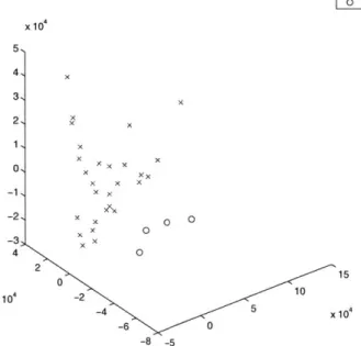
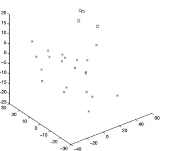
The visualizations of the pancreas data set seem to indicate that there may be a possible misclassification of single "normal" sample, which is consistently among a subset of the cancer samples. Also bothersome is the complete dispersion of the cancer samples. There is no tight cluster of cancer samples.

Overall, most of the data sets (especially the lung data set) are well suited for analysis. The cancer and normal samples cluster well respectively, and there is a reasonably specific dividing line between the two clusters. Now that it is established that most of the data sets contain genomic measurements that separate the cancer

Tissue Type using MDS 3-d plot using LLE 3-d plot

breast possibly possibly

colon yes possibly

gastric yes yes

kidney possibly possibly

liver no no

lung yes yes

ovary possibly yes

pancreas NO NO

MDS into 3 Dimensions of 10 pancreas samples x cancerous sample 0 non-cancerous sample x 104 4, 3, 2, 1 0 x x x 0 x x 01 -1, -2, -3, -4 4 2 S00.5 x104 -2 0 -0.5 x 10 _1 -6 -1.5

Figure 3-7. Possible misclassified sample

and normal samples, feature space reduction techniques are required to identify those genes that cause this separation.