The sensitivity of aerosol in Europe to two different emission inventories and temporal distribution of emissions

(1)

HAL Id: hal-00296034

https://hal.archives-ouvertes.fr/hal-00296034

Submitted on 25 Sep 2006

HAL is a multi-disciplinary open access

archive for the deposit and dissemination of

sci-entific research documents, whether they are

pub-lished or not. The documents may come from

teaching and research institutions in France or

abroad, or from public or private research centers.

L’archive ouverte pluridisciplinaire HAL, est

destinée au dépôt et à la diffusion de documents

scientifiques de niveau recherche, publiés ou non,

émanant des établissements d’enseignement et de

recherche français ou étrangers, des laboratoires

publics ou privés.

emission inventories and temporal distribution of

emissions

A. de Meij, M. Krol, F. Dentener, E. Vignati, C. Cuvelier, P. Thunis

To cite this version:

A. de Meij, M. Krol, F. Dentener, E. Vignati, C. Cuvelier, et al.. The sensitivity of aerosol in Europe

to two different emission inventories and temporal distribution of emissions. Atmospheric Chemistry

and Physics, European Geosciences Union, 2006, 6 (12), pp.4287-4309. �hal-00296034�

(2)

www.atmos-chem-phys.net/6/4287/2006/ © Author(s) 2006. This work is licensed under a Creative Commons License.

Chemistry

and Physics

The sensitivity of aerosol in Europe to two different emission

inventories and temporal distribution of emissions

A. de Meij1, M. Krol1,*, F. Dentener1, E. Vignati1, C. Cuvelier1, and P. Thunis1

1_{Institute for Environment and Sustainability, Joint Research Centre, European Commission, Ispra, Italy} *_{now at: SRON, Utrecht, the Netherlands, and Wageningen University, The Netherlands}

Received: 7 December 2005 – Published in Atmos. Chem. Phys. Discuss.: 18 April 2006 Revised: 11 July 2006 – Accepted: 18 September 2006 – Published: 25 September 2006

Abstract. The sensitivity to two different emission

inven-tories, injection altitude and temporal variations of anthro-pogenic emissions in aerosol modelling is studied, using the two way nested global transport chemistry model TM5 fo-cussing on Europe in June and December 2000. The simu-lations of gas and aerosol concentrations and aerosol optical depth (AOD) with the EMEP and AEROCOM emission in-ventories are compared with EMEP gas and aerosol surface based measurements, AERONET sun photometers retrievals and MODIS satellite data.

For the aerosol precursor gases SO2 and NOx in both months the model results calculated with the EMEP inven-tory agree better (overestimated by a factor 1.3 for both SO2 and NOx) with the EMEP measurements than the simulation with the AEROCOM inventory (overestimated by a factor 2.4 and 1.9, respectively).

Besides the differences in total emissions between the two inventories, an important role is also played by the vertical distribution of SO2and NOxemissions in understanding the differences between the EMEP and AEROCOM inventories. In December NOx and SO2from both simulations agree within 50% with observations.

In June SO=₄ evaluated with the EMEP emission inventory agrees slightly better with surface observations than the AE-ROCOM simulation, whereas in December the use of both inventories results in an underestimate of SO4 with a factor 2. Nitrate aerosol measured in summer is not reliable, however in December nitrate aerosol calculations with the EMEP and AEROCOM emissions agree with 30%, and 60%, respec-tively with the filter measurements. Differences are caused by the total emissions and the temporal distribution of the aerosol precursor gases NOxand NH3. Despite these differ-ences, we show that the column integrated AOD is less sensi-tive to the underlying emission inventories. Calculated AOD

Correspondence to: A. de Meij

([email protected])

values with both emission inventories underestimate the ob-served AERONET AOD values by 20–30%, whereas a case study using MODIS data shows a high spatial agreement.

Our evaluation of the role of temporal distribution of an-thropogenic emissions on aerosol calculations shows that the daily and weekly temporal distributions of the emissions are only important for NOx, NH3and aerosol nitrate. However, for all aerosol species SO=₄, NH+₄, POM, BC, as well as for AOD, the seasonal temporal variations used in the emission inventory are important. Our study shows the value of in-cluding at least seasonal information on anthropogenic emis-sions, although from a comparison with a range of measure-ments it is often difficult to firmly identify the superiority of specific emission inventories, since other modelling un-certainties, e.g. related to transport, aerosol removal, water uptake, and model resolution, play a dominant role.

1 Introduction

Greenhouse gases and aerosols play an important role in climate change (Charlson et al., 1991; Kiehl and Briegleb, 1993). Greenhouse gases reduce the emission of long wave radiation back to space, leading to a warming of the at-mosphere. Aerosol can change the atmosphere’s radiation budget by reflecting or absorbing incoming radiation (direct effect) and by modifying cloud properties (indirect effect). Quantification of the role of aerosols on the Earth’s radia-tion balance is more complex than for greenhouse gases, be-cause aerosol mass and particle number concentrations are highly variable in space and time, and the optical properties of aerosol are uncertain.

A good estimate of the emissions of aerosol precursor gases and primary aerosols in the emission inventories is therefore crucial for estimating aerosol impacts on air quality and climate change, and evaluating coherent reduction strate-gies.

(3)

Two major uncertainties of the current regional and global scale emission inventories comprise the accurate estimation of the quantity of the aerosols and precursor emissions, and the role of the temporal distribution of the emissions in the inventories.

Whereas some work on the impact of the temporal distri-bution of emissions on photochemistry in regional and urban areas has been performed (e.g. Pont and Fontan, 2001; Pryor and Steyn, 1995; Jenkin et al., 2002), to our knowledge no studies have been devoted to evaluate its impact on aerosol surface concentrations and mid-visible aerosol optical depths (AODs). The latter is an important parameter that is needed to calculate the Angstrom parameter, which provides infor-mation on the size of the particles in a given atmospheric column.

This study has two main objectives. The first objective is to evaluate uncertainties in gas, aerosol and aerosol optical depth calculations, resulting from two widely used emission inventories focussing on Europe. To this end we performed with the global transport chemistry TM5 model simulations using a zoom over Europe, for which we had two differ-ent emission invdiffer-entories available, EMEP and AEROCOM. The European scale EMEP inventory has been used for many years in the evaluation of emission reduction strategies, and contains reported emissions by member countries, as well as expert estimates. The AEROCOM project provided a com-pilation of recommended global scale aerosol and precursor emission inventories for the year 2000 and was used in the recent AEROCOM global aerosol module intercomparison (Kinne et al., 2006; Textor et al., 2006; Dentener et al., 2006). The second objective is to evaluate the role of the tempo-ral and height distribution of the emissions on aerosol (pre-cursor) concentrations and AOD calculations. For this we performed simulations using the EMEP inventory, with the standard recommendations on the temporal distribution of emissions (including seasonal variability) and compared it to a simulation ignoring daily emissions variations and another simulation that used annual averaged emissions.

The model performance was evaluated comparing aerosol precursor gases (NOx, SO2, NH3)and aerosols components (SO=₄, NH+₄, NO−₃, black carbon (BC) and particulate or-ganic matter (POM)) to the EMEP network surface observa-tions and to AERONET and MODIS AOD focussing on June and December 2000, over Europe.

Section 2 deals with the description of the simulations, model and emission inventories. In Sect. 3 a description of the remote sensing data and measurement data is given. In Sect. 4 the results are presented. We discuss the results in Sect. 5 and we finish with conclusions in Sect. 6.

2 Methodology

Using the two way nested global chemistry transport model TM5, we performed four simulations for the year 2000.

Out-put was analyzed for a summer (June) and winter (Decem-ber) month to highlight the seasonal dependency of emis-sions and their interaction with the different meteorological conditions prevailing in summer and winter.

The first simulation (further denoted as SEMEP)uses the EMEP inventory for the European domain, including their temporal (including, daily, weekly and seasonal variability) and height distribution. The second simulation SAERO used the AEROCOM recommended emission inventory. The third simulation, SEMEP c, ignored the weekly and daily tempo-ral distribution of emissions, but seasonal tempotempo-ral distribu-tions are still included. Finally we performed a simulation for which a seasonally constant temporal distribution was imple-mented, SEMEP c annual.

2.1 The nested TM5 model

The TM5 model is an off-line global transport chemistry model (Bergamaschi et al., 2005; Krol et al., 2005; Peters et al., 2004) driven by meteorological ECMWF (European Centre for Medium-Range Weather Forecasts) data. The presently used configuration of TM5 has a spatial global res-olution of 6◦×4◦and a two-way zooming algorithm that al-lows resolving regions, e.g. Europe, Asia, N. America and Africa, with a finer resolution of 1◦×1◦. A domain of 3◦×2◦ has been added, to smooth the transition between the global and finer region. The zooming algorithm gives the advantage of a high resolution at measurement locations. The vertical structure has 25 hybrid sigma-pressure layers. In this study the 1◦×1◦resolution was used for Europe/North African re-gion spanning from 21◦W to 39◦E and from 12◦S to 66◦N. Transport, chemistry, deposition and emissions are solved using the operator splitting. The slopes advection scheme (Russel and Lerner, 1981) has been implemented and deep and shallow cumulus convection is parameterised according to Tiedtke (1989).

The gas phase chemistry is calculated using the CBM-IV chemical mechanism (Gery et al., 1989a, b) solved by means of the EBI (Eulerian Backward Iterative) method (Hertel et al., 1993), like in the parent TM3 model, which has been widely used in many global atmospheric chemistry studies (Houweling et al., 1998; Peters et al., 2002; Dentener et al., 2003). In the current model version CO, NMVOC, NH3, SO2 and NOx gas phase, and BC (black or elemental car-bon), POM (particulate organic matter), mineral dust, sea salt (externally mixed), SO=₄, NO−₃, NH+₄ aerosol components were included. Mineral dust and sea salt (SS) were described using a log-normal distribution (3 for SS, 2 for dust) and their aerosol number and mass were separately transported using a fixed standard deviation of the size distribution (Vi-gnati et al., 2005). The aerosol components SO=₄, methane sulfonic acid (MSA) NO−₃, NH+₄, POM, and BC, were in-cluded assuming that they were entirely present in the ac-cumulation mode and externally mixed. In this first aerosol version of TM5, aerosol dynamics (coagulation, nucleation,

(4)

condensation and evaporation) are not included. However, gas-aerosol equilibrium of inorganic salts and water up-take is considered using the Equilibrium Simplified Aerosol Model (EQSAM version v03d, Metzger, 2000; Metzger et al., 2002a, b). This model allows non-iterative calculation of the equilibrium partitioning of major aerosol compounds of the ammonia (NH4), nitric acid (NO3), sulphuric acid (SO4)and water system. EQSAM assumes internally mixed aerosols and that the water activity of an aqueous aerosol is equal to the ambient RH (relative humidity). Hence, aerosol water is a diagnostic rather than transported model parame-ter. Water uptake on SS, is calculated using the description of Gerber et al. (1985).

Formation of secondary organic aerosol was not explicitly described, but included as pseudo organic aerosol emissions for the AEROCOM simulation but not for the simulation us-ing EMEP emissions (see Sect. 2.3.2).

Dry deposition is parameterized according to Ganzeveld (1998). In-cloud as well as below-cloud wet removal are parameterized differently for convective and stratiform pre-cipitation, building on the work of Guelle et al. (1998), and Jeuken et al. (2001).

For BC and POM we assume 100% hydrophilic properties in our model, and hence we assume that BC/POM is removed by wet and dry depositional processes like soluble inorganic aerosol (SO=₄). TM5 utilized information from the 6-h IPS forecast on 3-D cloud cover and cloud liquid water content, convective and stratiform rainfall rates at the surface, and sur-face heat fluxes to calculated convection.

Removal by convective clouds is taken into account by re-moving aerosols and gases in convective updrafts- with a cor-rection for sub-grid effects on the larger model scale.

Removal by stratiform clouds considers precipitation for-mation and evaporation, and cloud cover, and takes into ac-count a grid-dependency. Effectively rain-out on smaller grids works more effectively than on larger grids. Removal of gases further take their Henry solubility into account. For aerosol we used an in-cloud wet removal efficiency of 70% for the soluble aerosols and a below cloud removal efficiency of 100%. Sedimentation was only taken into account for dust and sea salt (large particles) and is considered to be negligi-ble for the sub-micron accumulation mode.

2.2 Aerosol size distribution and AOD calculation

For optical calculations, the accumulation mode aerosol, comprising sulphate, nitrate, ammonium, aerosol water, POM and BC, is described by a fixed Whitby lognormal dis-tribution, using a dry particle median radius of 0.034 µm and standard deviation (σ ) 2.0. As mentioned before, dust and sea salt are described with multi-model lognormal distribu-tion. Aerosol mass and number are transported separately, and as a consequence, the size distribution is allowed to change due to transport and deposition. Two modes are con-sidered for anthropogenic dust (accumulation, σ =1.59 and

coarse, σ =2.0) and three modes for sea salt (Aitken, σ =1.59, accumulation, σ =1.59 and coarse, σ = 2.0). As described be-fore, water uptake by the aerosol is taken into account and modify the above mentioned diameters.

To calculate aerosol optical depth (AOD) at 550 nm, we use the Mie code provided by O. Boucher (2004, personal communication) to pre-calculate a look-up table for a number of refractive indices and lognormal distributions. The optical properties of these lognormal distributions are determined by numerical interpolation in discrete size intervals corre-sponding to the median diameter. In Table S1 of the elec-tronic supplement (ES, http://www.atmos-chem-phys.net/6/ 4287/2006/acp-6-4287-2006-supplement.pdf) the densities and optical properties that are used for the optical calcula-tions are listed.

2.3 Emission data

In this study we used two independent emission invento-ries for aerosol and aerosol precursor gases for the year 2000. (i) The 50 km×50 km European scale EMEP in-ventory, which is widely used for air quality studies in Europe, and (ii) the 1◦×1◦ global AEROCOM inventory, which is used for climate modelling studies. Below, a brief description of the two emission inventories is given, to-gether with the major differences between the two inven-tories. In ES Table S2 (http://www.atmos-chem-phys.net/ 6/4287/2006/acp-6-4287-2006-supplement.pdf), we present an overview of the species which are included in the two emission inventories.

2.3.1 EMEP emission inventory

The Co-operative Programme for Monitoring and Evaluation of the Long-range Transmission of Air Pollutants in Europe (EMEP) evaluates air quality in Europe by operating a mea-surement network, as well as performing model assessments. The EMEP emission inventory (http://aqm.jrc.it/eurodelta and http://webdab.emep.int/) contains reported anthro-pogenic emission data for each European country, comple-mented by expert judgements when incomplete or erroneous data reports are detected. The 50 km×50 km emission in-ventory contains SO2, NOx(as NO2), NH3, NMVOC, CO, PM2.5 and PMcoarse for 11 CORINAIR source sectors. The emissions are temporally distributed per source sector us-ing time factors. We consider hourly (a multiplication fac-tor that changes each hour and modifies the daily emission), daily (a factor that changes the weekly emissions) and sea-sonally (a factor that changes each month, thus altering the seasonal distribution). For instance, it is important for traf-fic to include rush-hours and weekday-weekend driving pat-terns, and also the intensity of domestic heating differs from winter to summer. To match the PM2.5 emissions with the components used in TM5 we assumed the following mass fractions: POM 35%, anthropogenic dust 15%, BC 25% and

(5)

sulphate 25%, based on Putaud et al. (2003). PM coarse is assumed to contain dust only. We added from the global AEROCOM emission inventory biomass burning, natural dust, sea salt and volcanic emissions for the year 2000 (see Sect. 2.3.2). Outside Europe we also use the AEROCOM inventory. ES Table S3 (http://www.atmos-chem-phys.net/ 6/4287/2006/acp-6-4287-2006-supplement.pdf) provides an overview of the 11 CORINAIR source sectors, together with the emissions per sector. Gas and PM emissions are dis-tributed to different height levels based on the sector they belong to. Point sources and volcanoes are added to the appropriate height, see ES Table S4. Note that unlike for the AEROCOM inventory, we did not consider pseudo-SOA emissions.

2.3.2 AEROCOM emission inventory

AEROCOM (an AEROsol module inter-COMparison in global models, see http://nansen.ipsl.jussieu.fr/AEROCOM) evaluates aerosol concentrations, optical properties, and re-moval processes in 21 global models (Kinne et al., 2006; Textor et al., 2006). AEROCOM experiment B aims at con-straining the models by providing a prescribed set of global natural and anthropogenic emissions for the year 2000. We briefly call this ad-hoc compilation of the best inventories that was available in the year 2003 the AEROCOM inven-tory, ftp://ftp.ei.jrc.it/pub/Aerocom (Dentener et al., 2006).

Monthly varying large scale biomass burning emissions of POM, BC and SO2 are based on GFED 2000 (Global Fire Emissions Database) (Van der Werf et al., 2003). Global emissions amount to 34.7 Tg, 3.06 Tg and 4.11 Tg (SO2), respectively. Fossil fuel/bio fuel related POM (12.3 Tg POM/yr) and BC (4.6 Tg C/year) emissions are based on Bond et al. (2004). Country and region based SO2 emis-sions for the year 2000 are provided by IIASA (Dentener et al., 2006; Cofala et al., 2005) and geographically dis-tributed with the EDGAR3.2 1995 data base. Global emis-sions amount to 138.3 Tg SO2/year and 3.5 Tg SO4/year. Natural emissions of SO2(e.g. volcanoes) are an update of the GEIA recommended datasets.

Daily averaged DMS emissions were taken from the LMDZ model (O. Boucher, 2003, personal communication) using the DMS surface water concentrations of Kettle and Andreae (2000) and the horizontal wind speed (Nightingale et al., 2000). Yearly DMS amount to 20.8 TgS. Daily sea salt emissions were taken from Gong (2002, 2003a, b), interpo-lated to a three modal distribution with a cut-off at r=10 µm, resulting in 8356 Tg/year. Similarly, daily dust emissions for 2000 are based on Ginoux (2004), were interpolated to 2 log-normal modes, corresponding to a global total of 1681 Tg/yr. Secondary organic aerosol is an important component of the aerosol system (Kanakidou et al., 2005). Since most AEROCOM models did not include a description of the formation of SOA (Secondary Organic Aerosol), and there are major difficulties to describe the formation

pro-cesses of SOA, AEROCOM therefore made the simpli-fying assumption that 15% of natural terpene emissions form SOA, altogether amounting to 19.11 Tg POM/year. In the TM5 model most other anthropogenic emissions such as NOx are taken from the EDGAR3.2 (1995) database, http://www.mnp.nl/edgar. NH3 emissions were based on Bouwman et al. (1997, 2002), and distributed using the hours of daylight per month after Dentener and Crutzen (1994). For the other components the yearly emissions are equally distributed over the year with no seasonal vari-ations. ES Table S5 (http://www.atmos-chem-phys.net/6/ 4287/2006/acp-6-4287-2006-supplement.pdf) includes the height of the emissions which are applied in the AEROCOM emission inventory.

2.3.3 EMEP emission inventory versus AEROCOM emis-sion inventory

There are substantial differences between the two emission inventories in describing BC, dust, POM, and sulphate emis-sions. The EMEP inventory contains detailed country based knowledge on a 50×50 km resolution, while the AEROCOM inventory offers the advantage of global consistency. EMEP reports PM2.5 emissions, which were disaggregated by us into individual aerosol components. For example, we as-sume that 25% and 35% of the PM2.5 emissions consists of BC and POM, while the AEROCOM BC and POM emis-sions are based on a technology based global inventory of black carbon emissions from fossil fuel and bio-fuel com-bustion (Bond et al., 2004). 15% of the EMEP PM2.5 is assumed to be anthropogenic dust (e.g. vehicular movements causing re-suspension of particles), while AEROCOM con-tains only natural dust emissions (Ginoux et al., 2004). Par-ticularly relevant for this study are the emissions from the Sahara. Finally, we assume that the remaining 25% of the EMEP PM2.5 emissions is primary sulphate. In the AERO-COM simulation we assume that 2.5% of all SOxof the AE-ROCOM emissions is emitted as primary sulphate. These different procedures result for the European domain in dif-ferent primary sulphate emissions of 0.22 and 0.23 Tg/year, respectively.

Focussing on the European domain, we give in ES Table S6 (http://www.atmos-chem-phys.net/6/4287/2006/ acp-6-4287-2006-supplement.pdf) an overview of the result-ing total emissions of NOx, CO, SO2, NH3, SO4, sea salt, BC, POM and dust included in the two inventories for Eu-rope in June, December and the annual amount.

The annual emissions of the two inventories are generally within 20%, however the annual AEROCOM POM emis-sions are higher by 45%, NH3 by 37% and mineral dust by 34%. The difference between the European scale NH3 AE-ROCOM (6.0 Tg) and EMEP (4.4 Tg) emissions stems likely from the recent NH3emission abatement measures to combat eutrophication problems in Northern Europe. These are cluded in the EMEP, but not in the Bouwman et al. (2002)

(6)

in-ventory. The much larger POM emissions in the AEROCOM inventory are due to the presence of SOA pseudo-emissions, which were not included in the EMEP emission inventory.

The differences in dust emissions are only due to the an-thropogenic dust sources from agriculture and transport in-cluded in the EMEP inventory. These emissions are added to the natural mineral dust from AEROCOM which was in-cluded in both inventories.

Larger differences appear in June, where we see that AE-ROCOM emissions of NOx, SO2, SO4, NH3, and POM are higher by 39%, 18%, 31%, 67% and 248%, respectively. Ex-cept for POM, these differences are mainly due to the sea-sonal time factors which are applied to the EMEP inventory only.

For December (ES Table S6, http: //www.atmos-chem-phys.net/6/4287/2006/

acp-6-4287-2006-supplement.pdf) the above mentioned discrepancies are smaller than in June, due to compen-sating effect of the seasonal distribution and the yearly discrepancies of the two inventories.

3 Description measurement data sets

For evaluation of the computed gas and aerosol concentra-tions we compare with EMEP measurements of SO2, NOx, and aerosol components. Model calculated AOD is com-pared with sun photometer data from the AERONET stations located in Europe, and MODIS (Moderate Resolution Imag-ing Spectro radiometer) satellite data.

The EMEP air quality monitoring network measures since the late 1970s ozone, heavy metals, Persistent Organic Pollu-tants (POPs), Volatile Organic Compounds (VOC) and par-ticulate matter (PM2.5, PM10, SO=₄, NO−₃ and NH+)₄ at ca. 150 sites in Europe. The aerosols are measured with a daily time resolution; SO2and NOxare reported hourly. Not every station measures all components, therefore the num-ber of EMEP stations available for comparison with model results differs per component.

One of the artefacts occurring with the main filter type (quartz) used by most EMEP stations is the evaporation of ammonium nitrate at higher temperatures. Tempera-tures exceeding 20◦C cause complete NH4NO3 evapora-tion from the quartz filter, a loss of 100%; and a loss of about 25% for NH+₄, based on 5–10 µg/m3 NO−₃ and 10– 20 µg/m3SO=₄ at Ispra during a summer month (ratio 2:1 for (NH4)2SO4/NH4NO3).

Temperatures between 20 and 25◦C cloud lead to a loss of 50% of the nitrate aerosol (Schaap et al., 2003a, b). There-fore almost all reported summer NH4NO3and NH+4 concen-trations present only a lower limit, rather than a realistic con-centration.

The AERONET (AErosol RObotic NETwork) Cimel sun photometers (Holben et al., 1998) used in this study are given in ES Table S7 (http://www.atmos-chem-phys.net/6/4287/

2006/acp-6-4287-2006-supplement.pdf). Due to cloudiness not all days of June and December could be used for aerosol retrieval. The sun photometer measures (every 15 min) in a 1.2◦field of view, at eight solar spectral bands (340, 380, 440, 500, 670, 870, 940 and 1020 nm). These solar extinction measurements are used to calculate for each wavelength the aerosol optical depth, with an accuracy of ±0.01–0.02 (Eck et al., 1999). Sun photometer acquires aerosol data only dur-ing daylight and in cloud free conditions. In this work the cloud screened and quality-assured level 2 data are used.

We used AOD at 550 nm, calculated from the AOD val-ues reported at 870 and 440 nm, using the information on the Angstr¨om coefficient (S. Kinne, personal communica-tion, 2004).

The MODIS (Moderate Resolution Imaging Spectro ra-diometer) on board of NASA’s Terra Earth Observing Sys-tem (EOS) mission retrieves aerosol over land (Kaufman et al., 1997) and ocean (Tanr´e et al., 1997) at high resolution. MODIS has one NADIR looking camera which retrieves data in 36 spectral bands, from 0.4 µm—14.5 µm with spa-tial resolutions of 250 m (bands 1–2), 500 m (bands 3–7) and 1000 m (bands 8–36). Daily level 2 (MOD04) aerosol optical thickness data are produced at the spatial resolu-tion of 10×10 km over land, aggregated from the original 1 km×1 km pixel size. As the swath width is about 2330 km, the instrument has almost a daily global coverage. Uncer-tainties in the MODIS products over land are relatively large. High albedo areas like the Sahara Desert and snow/ice cov-ered regions and complex terrain are difficult for the MODIS instrument, leading to a large bias with models and ground based observations (Chin et al., 2004). Reported MODIS aerosol errors are 1τa=±0.05±0.15τa(Remer et al., 2005).

Level 2 cloud screened, version 003 files are used for this work. We present in Sect. 4 a case study for the 11 June 2000.

4 Results

In this section we present first an evaluation of the im-pact of using the EMEP and AEROCOM inventories (SEMEP and SAERO)and compare them with EMEP measurements (Sect. 4.1). In Sect. 4.2 we subsequently demonstrate the spatial variability of AOD associated with using these two emissions inventories, and compare it to MODIS retrievals. In Sect. 4.3 we assess the temporal variability of AOD by comparing to AERONET sun photometer data. Finally in Sect. 4.4, we perform two sensitivity studies to analyse the impact of daily, weekly and seasonal temporal distribution of emissions on gas, aerosol and AOD calculations. For the interested reader, detailed station information and statistics per component are presented in the accompanied electronic supplement to this paper.

(7)

(a)

Mean SO2 EMEP JUNE

0.0 0.2 0.4 0.7 0.9 1.1 1.3 1.6 1.8 2.0 ppb

Correlation stations: 0.83 / Best fit: y = 1.31x

0 1 2 3

Measured mean concentration 0

1 2 3

Modeled mean concentration

FI37 GB06 GB13 GB16 IT04 NL10 NO01 NO08 SE08 (b)

Mean SO2 AEROCOM JUNE

0.0 0.2 0.4 0.7 0.9 1.1 1.3 1.6 1.8 2.0 ppb

0 1 2 3

Measured mean concentration 0

1 2 3

FI37 GB06 GB13 GB16 IT04 NL10 NO01 NO08 SE08

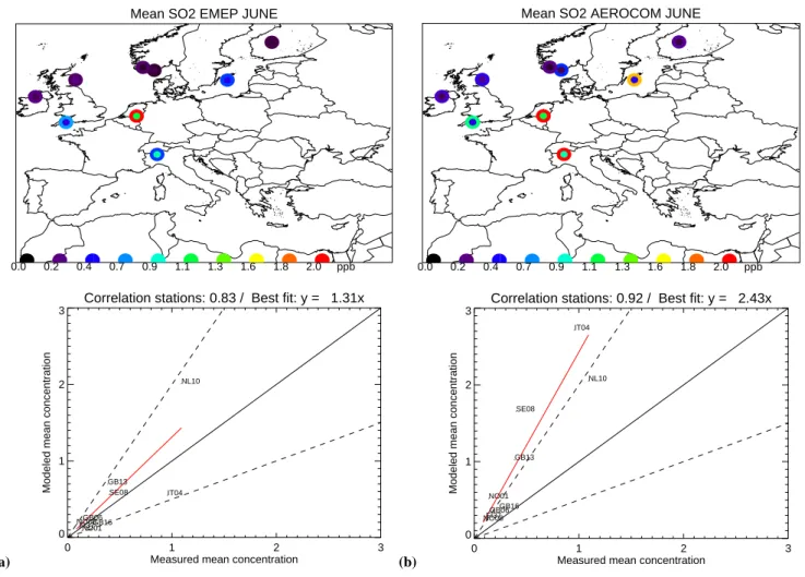
Fig. 1. (a), (b), (c) and (d) are presenting the monthly average measured mixing ratio (inner circle) of SO2and calculated (outer circle) SO2

by SEMEPand SAEROfor June and December 2000. For reference, the 2:1 and 1:2 lines are shown as the dashed lines, the 1:1 line as solid

and the line of best fit is red solid.

4.1 Evaluation of SEMEPand SAERO with surface observa-tions

In order to compare EMEP station data with model results on a 1◦×1◦ grid, we selected those measurement stations able to represent the model spatial scale and which had suffi-ciently data completeness for the month under consideration. First we compare daily average concentrations modelled at the EMEP stations to the measurement data. If the temporal correlation between the time series (with a data complete-ness of at least 10 days/month) is less than 0.5 (either in SEMEP and SAERO), due to measurement errors and sparse data availability, we excluded the stations from the analysis. An other possible reason for bad correlation between model and measurements, is that apparently the sub-grid scale local meteorology can not be accurately described by the resolu-tion (1◦_×₁◦_{) of the model.}

This procedure allows a fair comparison between mea-sured and modelled concentrations. Subsequently we

de-termined the spatial correlation using the monthly averaged concentration, and calculate the model bias.

We evaluate the sulphate and nitrate aerosol precursor gases SO2, and NOx, and the aerosol components SO=₄, NO−₃, NH+₄ and BC. The overall evaluation is presented in Figs. 1, 2 and 3, which shows the monthly mean concentra-tion distribuconcentra-tion over Europe.

4.1.1 SO2

In Figs. 1a–d we present an evaluation of SEMEP and SAERO computed SO2 concentrations. In June, both sim-ulations show high spatial correlation coefficients, of 0.83 and 0.92, respectively (based on 9 stations, 68 station re-jected). The June mean SO2concentrations for SEMEP are in better agreement (an overestimate of 31%) with the mea-sured values than SAERO (an overestimate by a factor 2.4). This discrepancy can not be explained by differences in the emissions alone, since the AEROCOM emissions of SO2 are only 18% higher over Europe than the EMEP

(8)

inven-(c)

Mean SO2 EMEP DEC

0.0 1.1 2.2 3.3 4.4 5.6 6.7 7.8 8.9 10.0 ppb

0 2 4 6 8 10

Measured mean concentration 0 2 4 6 8 10

AT02 DK03 FI17 FI37 GB06 GB13 GB15 NL10 PL02 PL05 SE08 YU05 (d)

Mean SO2 AEROCOM DEC

0.0 1.1 2.2 3.3 4.4 5.6 6.7 7.8 8.9 10.0 ppb

0 2 4 6 8 10

Measured mean concentration 0 2 4 6 8 10

AT02 DK03 FI17 FI37 GB06 GB13 GB15 NL10 PL02 PL05 SE08 YU05 Fig. 1. Continued.

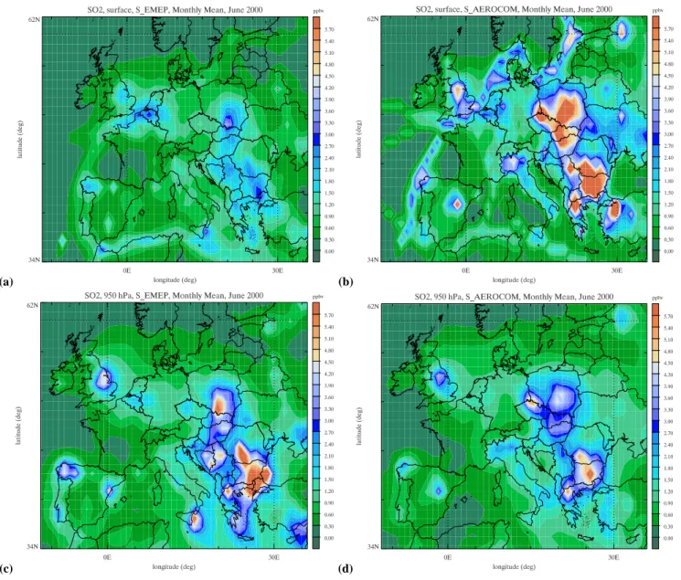
tory (ES Table S6, http://www.atmos-chem-phys.net/6/4287/ 2006/acp-6-4287-2006-supplement.pdf). A likely explana-tion lies in the vertical distribuexplana-tion of the emissions applied in the inventories (ES Tables S4 and S5). For that reason we present in Figs. 2a and b the June mean SO2 surface con-centrations. Especially in the eastern part of Europe the SO2 concentrations by SAEROat ground level are up to a factor of 2 higher due to the higher fraction of emissions in the low-est model layer. When we compare the SO2distributions at 950 hPa (±500 m, Figa. 2c and d) we observe especially in Eastern Europe an opposite situation; smaller SO2emissions from domestic heating (contributing by 6.8% to all emis-sions). In SAEROSO2is emitted at ground level only, which could be held responsible for the higher SO2 concentrations at ground level, where in EMEP 50% of SO2is emitted at a higher level.

For December the difference between the SO2calculations by SEMEP and SAERO is much smaller, see Figs. 1c and d (based on 12 stations used and 66 rejected). On a monthly averaged basis SEMEP concentrations are 2% lower than the measurements, with a spatial correlation coefficient of 0.91.

SAERO overestimates the measurements with 47% and has a high spatial correlation of 0.94. Note that the high corre-lation coefficients are statistically not robust (Figs. 1c and d), since they are determined by a few stations with a high spread in the monthly mean concentrations. The better agree-ment for the two simulations in December is in line with the smaller differences (2%) between the two emission inven-tories (see ES Table S6, http://www.atmos-chem-phys.net/ 6/4287/2006/acp-6-4287-2006-supplement.pdf). Tables S9a and S9b of the electronic supplement contain for each station the calculated monthly mean and correlation coefficients for SEMEPand SAEROtogether with the measured monthly mean and the number of measurements for June and December. 4.1.2 NOx

In June, SEMEPslightly overestimates (by 28%) the monthly mean NOx values, while the SAERO simulation overes-timates NOx by a factor of 1.95 (not shown). Spa-tial correlation coefficients are 0.79 and 0.53, respec-tively (based on 11 stations, 49 rejected). The difference

(9)

(a) (b)

(c) (d)

Fig. 2. Monthly SO2distribution by SEMEPand the SAEROat surface level (a and b, respectively) and 950 hPa (c and d, respectively) for

June 2000.

can be partly explained by the overall higher (39%, ES Table S6, http://www.atmos-chem-phys.net/6/4287/2006/ acp-6-4287-2006-supplement.pdf) monthly emissions in the AEROCOM inventory compared to EMEP. However, the stations available for comparison with measurements seem heavily biased to Northern Europe, where indeed the spa-tial difference between the EMEP and AEROCOM inventory seems higher. The vertical distribution plays also here an im-portant role. The monthly mean NOxsurface concentrations by SAERO are up to a factor of 2 higher in the Northern part of Europe, due to higher emissions in the lowest model layer (not shown). The differences in monthly mean NOx concen-trations at ±500 m between SAEROand SEMEPare smaller.

In December, SEMEP and SAERO NOx mean con-centrations are closer to the measurements, and are respectively 7% and 11% higher (see ES Ta-ble S10b, http://www.atmos-chem-phys.net/6/4287/2006/ acp-6-4287-2006-supplement.pdf). Spatial correlations are 0.76 and 0.79 for SEMEP and SAERO, respectively (based on 17 stations, 43 rejected).

4.1.3 SO=₄

Figures 3a–d present the EMEP measured and modelled (SEMEP and SAERO)SO=4 concentrations for June and De-cember 2000. Spatial correlation coefficients are compara-ble for SEMEP(0.66) and SAERO(0.65) (based on 38 stations

(10)

(a)

Mean SO4 EMEP JUNE

0.0 0.2 0.4 0.7 0.9 1.1 1.3 1.6 1.8 2.0 ppb

0.0 0.5 1.0 1.5 2.0

Measured mean concentration 0.0

0.5 1.0 1.5 2.0

AT02 CH05 ES04 ES11 FI09 FI17 FI37 FR05 FR09 FR10 FR13 GB02 GB04 GB06 GB07 GB13 GB14 GB15 GB16 HU02 IE03 IE04 LT15 NL09 NL10 NO01 NO08 NO39 NO41 PL02 PL04 PL05 RU16 RU18 SE02 SK04 SK05 TR01 (b)

Mean SO4 AEROCOM JUNE

0.0 0.2 0.4 0.7 0.9 1.1 1.3 1.6 1.8 2.0 ppb

0.0 0.5 1.0 1.5 2.0

0.5 1.0 1.5 2.0

AT02 CH05 ES04 ES11 FI09 FI17 FI37 FR05 FR09 FR10 FR13 GB02 GB04 GB06 GB07 GB13 GB14 GB15 GB16 HU02 IE03 IE04 LT15 NL09 NL10 NO01 NO08 NO39 NO41 PL02 PL04 PL05 RU16 RU18 SE02 SK04 SK05 TR01

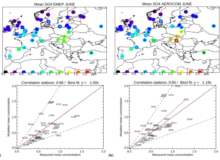
Fig. 3. (a), (b), (c) and (d) are presenting the monthly average measured mixing ratio (inner circle) of SO=₄ and calculated (outer circle) SO=₄ by SEMEPand SAEROfor June and December 2000. For reference, the 2:1 and 1:2 lines are shown as the dashed lines, the 1:1 line as

solid and the line of best fit is red solid.

used and 33 rejected). The modelled SO=₄ concentrations by SEMEPmatch the measurements while SAEROon average slightly overestimates SO=₄ aerosol concentrations by 19%. Especially over central Europe (Austria, Hungary, Czech Republic and Poland) significantly higher SO=₄ concentra-tions are calculated by SAERO than for SEMEP, which can be attributed to the higher over-all emissions. For Decem-ber the differences between the two simulations are rather small and both SEMEP and SAERO underestimate on av-erage the modelled SO=₄ aerosol concentrations compared with measurement data by as much as a factor 2 (based on 23 stations, 45 rejected). The wintertime underestima-tion of sulphate concentraunderestima-tions has been observed earlier and is possibly due to a lack of oxidation chemistry in the model (Jeuken, 2000; Kasibhatla et al., 1997). More de-tailed information in Tables S11a and S11b of the electronic supplement (http://www.atmos-chem-phys.net/6/4287/2006/ acp-6-4287-2006-supplement.pdf).

4.1.4 NO−₃

Since in summer EMEP measurements have serious mea-surement artefacts (see Sect. 3) we can only analyse dif-ferences between nitrate aerosol computed by SEMEP and SAERO for December. Substantial differences are found for NO−₃ aerosol: SAERO calculates a maximum concentration of 22.1 µg/m3 over Germany, while the SEMEP calculated maximum amounts to 9.6 µg/m3. Over Poland SAERO cal-culates NO−₃ aerosol values of 5 µg/m3, while SEMEP calcu-lates NO−₃ aerosol <2 µg/m3. The higher NO−₃ found with the AEROCOM inventory, can be understood from higher NOx(+39%) and NH3(+67%) emissions in the AEROCOM (taken from EDGAR3.2 database) than in the EMEP inven-tory.

Reactions (1–4) show how NO−₃ aerosol formation is re-lated to both NOxand NH3emissions:

(11)

(c)

Mean SO4 EMEP DEC

0.0 0.1 0.2 0.3 0.4 0.6 0.7 0.8 0.9 1.0 ppb

0.0 0.5 1.0 1.5 2.0

0.5 1.0 1.5 2.0

PL05 CH02 ES04 ES09 ES12 ES13 ES15 FR03 _FR05 FR09 FR10 FR13 GB07 GB13 GB14 GB15 HU02 IT01 LT15 NL10 NO08 PL02 PL04 (d)

Mean SO4 AEROCOM DEC

0.0 0.1 0.2 0.3 0.4 0.6 0.7 0.8 0.9 1.0 ppb Correlation stations: 0.57 / Best fit: y = 0.48x

0.0 0.5 1.0 1.5 2.0

0.5 1.0 1.5 2.0

PL05 CH02 ES04 ES09 ES12 ES13 ES15 FR03 FR05 FR09 FR10 FR13 GB07 GB13 GB14 GB15 HU02 IT01 LT15 NL10 NO08 PL02 PL04 Fig. 3. Continued. and, NO2(g)+NO3(g)→N2O5 (R2) The hydrolysis of N2O5 on wet aerosol surfaces is an im-portant pathway to convert NOxinto HNO3 (Dentener and Crutzen, 1993; Riemer et al., 2003; Schaap et al., 2003a, b): N2O5(g)+H2O → 2HNO3 (R3) NH3(g)+HNO3(g)↔NH4NO3 (aq,s) (R4) For December SEMEPoverestimates measured aerosol nitrate by a factor of 1.37, and SAERO by a factor of 1.62. Ta-ble S12 in the ES (http://www.atmos-chem-phys.net/6/4287/ 2006/acp-6-4287-2006-supplement.pdf) shows that SAERO aerosol nitrate concentrations are at all stations higher than those of SEMEP (except for PL02). A possible explanation for these differences could be related to higher NH3 emis-sions (21% higher in winter) in the AEROCOM than in the EMEP inventory. High spatial correlation coefficients of 0.84 (EMEP) and 0.91 (AEROCOM) are found (based on 6 sta-tions, 15 rejected), indicating that the spatial gradients of the

monthly mean concentrations are relatively well reproduced by the model.

4.1.5 NH+₄

EMEP reports in many cases the sum of NH3and NH+4, also called total ammonium (NHx). For these cases we compared measurements to the modelled sum of the two components.

SEMEPNHxconcentrations agree well with measurements for June, and are on average only 4% higher. In con-trast, SAERO overestimates NHx on average by a factor of 2.0. Analyzing the monthly mean concentrations (ES Table S13a, http://www.atmos-chem-phys.net/6/4287/2006/ acp-6-4287-2006-supplement.pdf), we see that for all sta-tions the values are higher for SAEROthan for SEMEP(based on 20 stations, 17 rejected). The overestimation of SAERO can explained by the 67% higher summer NH3 emissions compared to the EMEP emission inventory. The spatial cor-relation coefficients are high with 0.81 and 0.80, respectively. For December SAERO agrees better with the measure-ments, and on average SAERO and SEMEP underestimate the

(12)

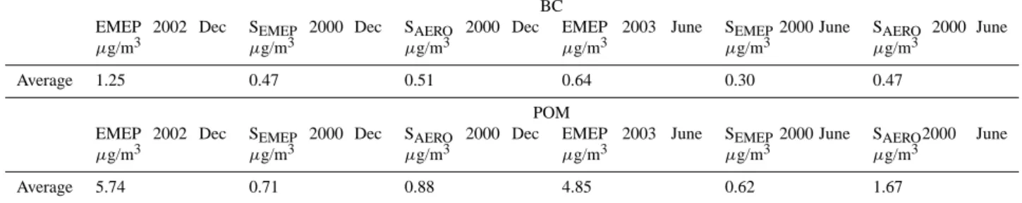
Table 1. Monthly mean BC and POM concentrations (µg/m3) for all the stations calculated by SEMEPand SAERO, together with EMEP

measurement data for December 2002 and June 2003.

BC EMEP 2002 Dec µg/m3 SEMEP 2000 Dec µg/m3 SAERO 2000 Dec µg/m3 EMEP 2003 June µg/m3 SEMEP2000 June µg/m3 SAERO 2000 June µg/m3 Average 1.25 0.47 0.51 0.64 0.30 0.47 POM EMEP 2002 Dec µg/m3 SEMEP 2000 Dec µg/m3 SAERO 2000 Dec µg/m3 EMEP 2003 June µg/m3 SEMEP2000 June µg/m3 SAERO2000 June µg/m3 Average 5.74 0.71 0.88 4.85 0.62 1.67

measured values with 7%, and 26%, respectively (based on 12 stations, 26 rejected). More detailed information per sta-tion in ES Table S13b .

4.1.6 BC

Unfortunately we have only one station (Ispra, Italy) to our disposal for comparison with black carbon (BC) simula-tions for the year 2000 (http://ccu.jrc.it/). Modelled mean BC concentration of 1.37 µg/m3 computed by SAERO is about 45% higher than the measured mean of 0.93 µg/m3 for June. In the same month, SEMEP underestimate BC by 33% (0.62 µg/m3). In December, the concentrations are 2.17 µg/m3, 1.42 µg/m3, and 1.90 µg/m3for SAERO, SEMEP and measurements, respectively. More BC measurements are available for 2002 and 2003. However, a quantitative com-parison with the 2000 simulations is difficult since the year-to-year variations can be large. For instance, EMEP mea-sured in Ispra for June 2002 a monthly mean of 1.38 µg/m3, compared to 0.93 µg/m3in June 2000. Nevertheless, to give an qualitative impression we present in Table 1 the average of the calculated BC concentrations of the 9 stations by SEMEP and SAERO and the EMEP measurement data for December 2002 and June 2003. BC concentrations for each station are given in ES Table S14a. For some stations the model corre-sponds very well with the measurements; in December with AT02, in June 2003 with AT02, DE02, FI17 and SE12. How-ever, at the majority of the stations the model underestimates BC concentrations, sometimes up to a factor of 7 (PT01). While the latter value may be influenced by wood burning for residential heating purposes. A possible explanation for these underestimations may be related to the uncertainties in the emission factors for BC in emission inventories, and unaccounted sources of BC which contribute to underesti-mation of BC in the emission inventories, as discussed by Schaap et al. (2004).

4.1.7 POM

Also for POM we have only one station (Ispra, Italy) to our disposal for model comparison for the year 2000. In June, the

monthly mean POM concentration by SAERO (2.35 µg/m3) is a factor of three higher than by SEMEP (0.70 µg/m3), because SOA emissions are included in the AEROCOM emission inventory, while for EMEP not. However POM by SAERO is still underestimated when compared to the measured monthly mean (3.00 µg/m3). In December the modelled monthly mean POM concentrations for SAERO and SEMEP are the same (1.43 µg/m3), but heavily under-estimated when compared to the measured monthly mean (9.59 µg/m3). More POM measurements are available for 2002 and 2003. As described above, a quantitative compar-ison with 2000 calculations can be difficult due to year-to-year variations. Also given in Table 1 is the average of the calculated POM concentrations of the 9 stations by SEMEP and SAERO and the EMEP measurement data for December 2002 and June 2003. POM concentrations for each station are given in ES Table S15 (http://www.atmos-chem-phys. net/6/4287/2006/acp-6-4287-2006-supplement.pdf).

In June 2000, POM concentrations by SAERO are for any station higher than by SEMEP, and agree better with measure-ment 2003 data, but still underestimated up to a factor of 5. In December the differences between SEMEPand SAERO are smaller and are for all the stations underestimated when compared to measurements.

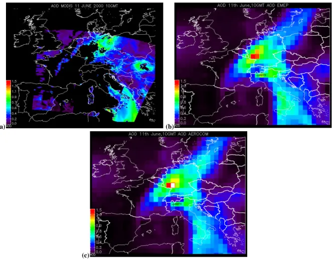
4.2 Case study of AOD over Europe on 11 June 2000 In this section we demonstrate the ability of our model to represent the spatial distribution of aerosol as seen from the MODIS satellite, by MODIS AOD retrieval for 11 June 2000. This specific event also allows evaluation of the factors de-termining spatial differences resulting from the use of the two inventories. This specific day was chosen, since it rep-resents a relatively cloud-free day throughout especially in central and eastern Europe, with heterogeneous contributions of desert dust intrusions in southern Europe and mixed pol-lution and dust in central and northern Europe.

The MODIS retrieved AOD is displayed in Fig. 4a. Three regions of high AOD (0.6–0.9) are observed: Southern Italy/Balkans, the Czech Republic/Romania, and North East

(13)

(a) (b)

(c)

Fig. 4. AOD over Europe for 11 June 10:00 GMT, 2000 by MODIS (a), AOD by SEMEP(b) and SAERO(c). White colours represent AOD

values larger than 1.5. Note that for aerosol equilibrium calculations an upper limit for RH 95% was used. No cloud masking was applied to model results.

MODIS MOD04 L2.A2000163.1035.004.2002365174903.hdf, variable optical Depth Land And Ocean is used.

Germany. Elsewhere the retrieved AOD was of the order of 0.1–0.2. It should be noted that in other parts of Europe no aerosol was reported, due to detection of clouds by the MODIS cloud screening algorithm. Over the southern part of Italy, MODIS registers small and large Angstrom coef-ficients, indicating that both coarse (dust) and fine particles are found in this region. Over the eastern part of Europe MODIS registers large Angstrom coefficients, which is typ-ical for small particles, e.g. inorganic sulphate- and nitrate aerosols.

With our CTM we can compare these observations with model calculated AOD, but additionally, with the model we are able to evaluate the contributions to AOD of single aerosol components. Figures 4b and c depicts the computed AOD distribution over Europe for 11 June 2000, 10:00 GMT for SEMEP and SAERO, respectively. We note here that the AOD calculations are based on the relative humidity in the cloud free part of the 1◦×1◦model grid-box (diagnosed from the grid-box average RH) and that the RH should not exceed

95%. However, clouds are not “masked” in our model cal-culations. To avoid calculations of highly uncertain RH in regions with almost complete cloud cover we discard the re-gions with ECMWF cloud cover larger than 90%. The distri-bution of AOD over Europe as calculated with the two inven-tories is very similar: maximum AOD values of 1.4 (SEMEP) and 1.6 (SAERO)are found over the western part of Germany, and bands of high AOD (0.6–0.9) are calculated over almost entire Germany, Austria, and Italy. Clean air travelling be-hind a frontal system in the western part of Europe, England, Denmark, the Netherlands, Belgium, France, and Spain is as-sociated with AOD smaller than 0.2. The high model AOD given by the two model simulations agrees very well with MODIS over Germany and Italy, but the high AOD retrieved over the Czech Republic/Romania is underestimated by the two model simulations. The model calculated AOD over Western Europe seems somewhat lower than the retrieved values.

(14)

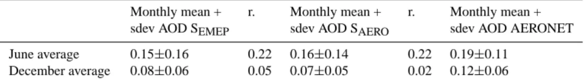
Table 2. Averaged AOD values together with the corresponding correlation coefficients for June and December 2000 for all the AERONET stations used in this work. The values are based on monthly mean AOD calculated by TM5 with the EMEP emission inventory and the AEROCOM emission inventory for each station.

Monthly mean + r. Monthly mean + r. Monthly mean + sdev AOD SEMEP sdev AOD SAERO sdev AOD AERONET

June average 0.15±0.16 0.22 0.16±0.14 0.22 0.19±0.11 December average 0.08±0.06 0.05 0.07±0.05 0.02 0.12±0.06

How do individual components contribute to the AOD?

A desegregation of individual components indicates that especially in the vicinity of Southern Italy, dust contributes with 0.15 (or 25%) to the AOD, which is in agreement with the MODIS observed Angstrom coefficients. In Northern Europe dust contributes with 0.05 to the computed AOD of 0.9. There the high computed AOD is caused by ele-vated concentrations of inorganic aerosols (SO=₄, NO−₃ and NH+₄)and associated aerosol water (aerosol water makes up to 70% of the total aerosol mass over this area). The pres-ence of small particulate inorganic aerosols in this area is found back in the Angstrom coefficients retrieved by MODIS which range from 2.5 to 4. According to the ECWMF mete-orological data underlying our model, high RH (>90%) and cloud cover around 70% prevail in the western part of Ger-many and high AOD is calculated due to the uptake of large amount of water by the inorganic aerosols. MODIS does not register AOD at all for this area, due to the reported presence of warm clouds. While this is consistent with the ECMWF meteorology, MODIS does probably often discard aerosol in the vicinity of regions with partial cloud cover and high RH.

As outlined in the previous section, the use of the AE-ROCOM emissions inventory leads to higher surface con-centrations of SO=₄ and NO−₃, because summertime emis-sions are higher. These differences are partially reflected in the calculated AOD. As mentioned above, the AOD ge-ographical patterns of SAERO and SEMEP are similar, but over the Baltic Sea AOD difference up to 0.4 are calcu-lated, due to higher SO=₄ concentrations over this area. In ES Table S11a (http://www.atmos-chem-phys.net/6/4287/2006/ acp-6-4287-2006-supplement.pdf) we see that higher SO=

4 concentrations are calculated by SAERO than by SEMEP (up to a factor of 2) for the Finish, Swedish and Lithuanian sta-tions. Over the southern part of Italy, higher AOD values are calculated by SEMEP, up to 0.2 difference. For this area SEMEPcalculates higher SO=₄ concentrations than SAERO, up to 9 µg/m3SO=₄ difference.

In the next section we will compare the calculated AOD values to AERONET measurements.

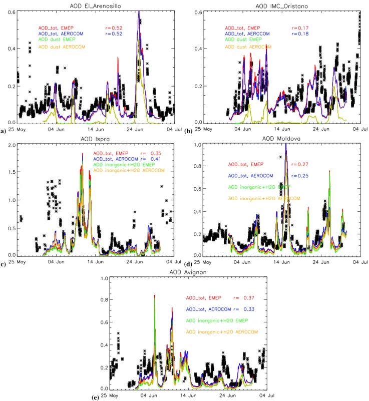
4.3 Comparison of modelled AOD with AERONET In this section we compare modelled AOD with the re-trieved AOD at a selected number of AERONET stations. While the geographic coverage of AERONET is rather lim-ited as compared to the satellite data described in the pre-vious section, we use the much higher time resolution to evaluate the temporal evolution of AOD in our model. To ensure monthly representativity we select for this compar-ison AERONET stations for which more than 50 observa-tions per month are reported; i.e. for June 9 staobserva-tions and for December only 6. An observation may represent a time span ranging from a few minutes to 15 min. The model out-put was sampled at station location at an hourly frequency. Table 2 present the average of the observed and computed (SEMEPand SAERO)monthly mean AOD for all stations, to-gether with the temporal correlation for June and December. In ES Tables S16 and S17 (http://www.atmos-chem-phys. net/6/4287/2006/acp-6-4287-2006-supplement.pdf) the ob-served and computed (SEMEP and SAERO) monthly mean AOD and their temporal correlation for each station is given for June and December 2000, respectively. Correlations be-tween model and measurement are rather low and range for individual stations between −0.04 and 0.52. On average the June AOD of SEMEP is 5% lower than the SAERO AOD and both simulations underestimate AERONET AOD by on av-erage 30%. Also for December both simulations underes-timate the AERONET AOD by 35%. To demonstrate the factors contributing to temporal variability we now focus in more detail on 5 stations in June (Figs. 5a–e) with a relatively large measurement records, and a widely varying geographic location: (i) El Arenosillo is a coastal site in Southern Spain (ii) Moldova is located in Eastern Europe, (iii) IMC Oristano is located on Sardinia in the Mediterranean Sea, (iv) Ispra is located at the foothills of the Alps in Northern Italy and (v) Avignon is located in the South/East part of France. Apart from the calculated AOD, we also show the contribution of the dominant aerosol component to AOD.

Modelled dust had a substantial contribution to the total AOD in El Arenosillo (Fig. 5a) around the 4, 9, 17–19, 25– 27 June. Indeed on these days high AOD were observed by AERONET (up to 0.55 on 26 June) and AERONET Angstrom coefficients ranged from 0.4–1.5, indicating the

(15)

presence of large dust particles. The monthly mean AOD val-ues calculated for both the emission inventories (0.09±0.11) are in line with the monthly mean AOD observed by AERONET 0.12 ±0.07 (ES Table S16). Temporal correla-tion coefficients of simulacorrela-tion and measurements are about 0.5. The high correlation is clearly caused by a correct tim-ing of the dust events by the model and similar in both simu-lations.

For IMC Oristano (Fig. 5b) we see again the large in-fluence of dust on AOD. AERONET AOD values goes up (>0.2) on days where the model calculates high dust loads. This is confirmed by the small Angstrom coefficients re-trieved for the days with high dust events (not shown). How-ever, the high observed and modelled AOD in the period 5–9 June seems unrelated to dust and caused by a large contri-bution of inorganic aerosol. Calculated monthly mean AOD values are about 0.15 and in agreement with AERONET re-trieved AOD of 0.15. The rather low time correlation appears to be the result of large diurnal variations in measured AOD which are not reproduced by the model.

At Ispra, two pollution events are visible in the measured AOD: 3–6 and 9–13 June.

The first pollution period could be an error in the cloud screening algorithm (G. Zibordi, personal communication, 2005) and is therefore neglected. However, consistent with observations, from the 9 to 13 June the model calculates a large contribution of inorganic aerosol to the total AOD (Fig. 5c). Note that AERONET reports cloud cover during parts of this event. We have seen in Sect. 4.2 that the model calculates high SO=₄ aerosol concentrations for this area (up to 20 µg/m3). During this episode, high relative humidity (RH) values of 76% were measured at the EMEP measure-ment station. ECMWF meteorological data used by TM5 showed average RH values of 82% for the same 5 day pe-riod. These high RH values in combination with high inor-ganic aerosol loads increase the uptake of water by aerosol, and hence AOD.

At Moldova (Fig. 5d), inorganic aerosol impacts the to-tal AOD in a similar way. High concentrations of inorganic aerosol together with high relative humidity cause high AOD values by AERONET and the model. One exception is en-countered on 21 June when the model calculates high AOD values (0.5) due to the presence of inorganic aerosol and high RH values (90%), where AERONET observes low AOD (0.08) values. The model calculates a monthly mean AOD of about 0.18, which is close to the monthly mean observed by AERONET.

The high AOD values calculated at Avignon (Fig. 5e) are caused by the high relative humidities together with high concentrations of inorganic aerosol, leading to AOD values up to 0.8. The model calculates a monthly mean AOD of about 0.10, which is about 30% lower than the monthly mean observed by AERONET (0.15).

Noticeable in all comparisons is the relatively small differ-ence between the SEMEPand SAEROAOD results, compared to the AERONET observed AOD. Apparently, the differ-ences observed close to the surface, quickly become smaller (or are even compensated) at some height, as was also ob-served in Figs. 2c and d for SO2and NOx. The height distri-bution of the emissions is obviously a less important factor for AOD values than for surface concentrations.

4.4 Temporal distribution of emissions

In the previous sections we evaluated the overall impact of the EMEP and AEROCOM emission inventories on aerosol (precursor) and AOD calculations. In this section we eval-uate uncertainties arising from the neglect of the temporal variations of the emissions. Apart from seasonal variations in emissions, this includes also variations on shorter time-scales, like diurnal, and day of week variations. Outside Europe and the USA this information is often not avail-able, which is one of the reasons that these variations are normally not included in global emission inventories of an-thropogenic emissions. To study the role of temporal vari-ation of emissions over Europe, we performed two addi-tional simulations. We compared SEMEP (including tem-poral variation factors) with SEMEP c, which uses constant hourly and daily emissions. In SEMEP c however, we re-tained the seasonal information on emissions. The im-portance of these seasonal variations was already shown in ES Table S6 (http://www.atmos-chem-phys.net/6/4287/ 2006/acp-6-4287-2006-supplement.pdf) where AEROCOM emissions in June appeared to be higher due to a lack in seasonal variation. In Sect. 4.4.2 we assess this issue again by comparing a simulation without seasonal variations (SEMEP c annual)with SEMEP c.

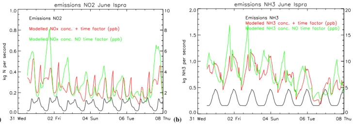
4.4.1 The impact of daily and weekly emission variations For short-lived species, like NOx and NH3, the short-term emission fluctuations are quite important. To illustrate this we show in Figs. 6a and b the temporal evolution of NO2and NH3 emissions, and the corresponding SEMEP and SEMEP c concentrations for Ispra (8.6◦E, 45.8◦N) for the period 1–8 June. At Ispra, the NO2 emission variations are dominated by a daily cycle, and the influence of weekend/working day emission variation is small, about 10%. There appears a strong co-variance of night-time stability and accumulation of NO2 emission in SEMEP cin the beginning of the week, dominated by fair weather conditions. During the second half of the week the differences are smaller because unstable meteorological conditions caused more vigorous mixing and advective transport. Similarly, NH3accumulation appeared in SEMEP c during the first part of the week, but not in the second (Fig. 6b). In December (not shown) these day-night differences in concentrations are much less, since the day-night contrast in atmospheric stability is smaller. NH3 and

(16)

(a) (b)

(c) (d)

(e)

Fig. 5. Total AOD of TM5 with EMEP emission inventory (red line) and AEROCOM emission inventory (blue line) and AERONET AOD (black stars), together with the AOD of the component which has the largest contribution to the total AOD, for El Arenosillo (a), IMC Oristano (b), Ispra (c), Moldova (d) and Avignon (e). Brown presents AOD by dust for AEROCOM (a, b) or inorganic aerosol and the associated water for (c–e). Green AOD by dust (a, b) or by inorganic aerosol and the associated aerosol water for (c–e).

NOx concentrations by SEMEP are in general lower than by SEMEP c.

We analyse in ES Table S18 the significance of this com-paring the modelled concentrations for the simulations with and without the temporal distribution, and when possible also

(17)

(a) (b)

Fig. 6. The temporal distribution of NO2(a) and NH3(b) emissions together with the modelled concentrations with and without temporal

variation, for Ispra, June 2000.

Table 3. Averaged concentrations and the corresponding standard deviation of all stations of the aerosol precursor gases NH₃and NOxfor

which the correlation coefficient for calculated NOxbetween SEMEPand SEMEP cin June is <0.8.

NH₃ppb NOxppb

SEMEP SEMEP C r SEMEP SEMEP C r EMEP data

June average 3.84±2.07 3.99±2.26 0.78 4.85±1.68 5.11±1.72 0.56 4.71±1.70 December

aver-age

2.60±1.85 2.54±1.70 0.85 9.37±6.40 9.36±6.22 0.94 8.53±4.09

with available observations. We analyzed the 14 EMEP mea-surement locations (44 rejected), for which the deviation be-tween the two simulations was found to be important (i.e. nearby regions of high emissions). The correlation coeffi-cient for calculated NOx between SEMEP and SEMEP c for these 14 stations in June is <0.8, indicating the importance of the daily and weekly distribution of the NOxemissions. The average concentrations of NH3and NOxfor all the sta-tions by SEMEPand SEMEP cfor June and December is given in Table 3.

For June the monthly averaged NH3and NOx concentra-tions are on average and in almost all cases somewhat lower when daily and weekly emission variations are taken into ac-count, up to 13% for NOx and 25% for NH3. Correlation coefficients of hourly modelled concentrations at the selected locations are between 0.29–0.74 for NOx, and between 0.65– 0.89 for NH3(ES Table S18a, http://www.atmos-chem-phys. net/6/4287/2006/acp-6-4287-2006-supplement.pdf). The re-sults of the modelled NOxconcentrations of both simulations agree on average very well with both observations.

We have very few representative NH3 measurement data available; e.g. for NH3in the Netherlands (NL10) calculated by SEMEPis lower (5.90 ppb) than by SEMEP c(6.42 ppb), but is for both cases far below the measured value of 23 ppb. At

HU02 NH3SEMEPis 3.01 ppb and NH3SEMEP cis 3.20 ppb, which agrees better to the measured mean concentration of 3.52 ppb. It seems that the spatial variability of measured NH3 is too large to prove that the modelled NH3improves when including high time resolution.

In December, SEMEP and SEMEP c, correlate on aver-age better than in June, and the concentrations deviate less strongly, indicating that also in other regions, in winter boundary layer mixing plays a less important role. Clearly including the hourly and daily emission-variability can not explain all model-measurement differences.

Differences in precursor concentrations (NH3, NOx)lead to differences in the calculated nitrate aerosol, which are smaller in all cases for SEMEP in June (up to 30%). In De-cember, when model results of SEMEP and SEMEP ccan be compared to artefact-free NO−₃ aerosol measurements (ES Table S19, 16 stations, including stations with temporal cor-relation coefficient smaller than 0.5) differences are rather small and do not lead to a clear improvement. For most longer-lived species the impact of daily and weekly emis-sions factors is smaller than 1–2%. The explanation for this observation is that for species that have a lifetime of more than a day, advective fluxes are dominating and mask the short-term emission variations.

(18)

Table 4. Averaged computed (SEMEPand SEMEP c)and observed NO−₃ aerosol concentrations, together with the corresponding temporal

correlation coefficient of all the stations, for December 2000.

December NO−₃ aerosol Monthly mean ppb SEMEP r Monthly mean ppb SEMEP C r EMEP ppb measurements December aver-age 1.40±0.93 0.45 1.41±0.92 0.44 0.93±0.62

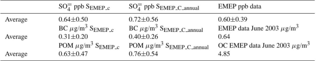
Table 5. Averaged computed (SEMEP cand SEMEP annual)and observed SO=4 aerosol, BC and POM concentrations and the corresponding

temporal correlation coefficient of all the stations, for June 2000.

SO=₄ ppb SEMEP c SO=4 ppb SEMEP C annual EMEP ppb data

Average 0.64±0.50 0.72±0.56 0.60±0.39

BC µg/m3SEMEP c BC µg/m3SEMEP C annual EMEP data June 2003 µg/m3

Average 0.31±0.20 0.40±0.26 0.64

POM µg/m3SEMEP c POM µg/m3SEMEP C annual OC EMEP data June 2003 µg/m3

Average 0.63±0.47 0.76±0.54 4.85

4.4.2 The impact of monthly emission variations

In this section we show that the seasonal distribution of emissions has a stronger impact on simulated SO=₄, BC and POM concentrations than the hourly and daily varia-tions. In our discussion we focus on June, similar effects but opposite in sign can be found for December. In ES Table S20 (http://www.atmos-chem-phys.net/6/4287/2006/ acp-6-4287-2006-supplement.pdf) we present the monthly mean concentrations for sulphate aerosol, BC and POM for June 2000. For BC and POM we compare measurement data of June 2003 (no measurement data available for 2000).

In June, the use of annual average emissions (SEMEP c annual) leads in general to higher emissions of e.g. SO2 and NOx, since the intensity of residential and commercial heating, is less during summer than in winter. As a consequence, aerosol and aerosol precursor concen-trations are generally higher in simulation SEMEP c annual. For instance, at Jarczew (PL02) the monthly mean SO2 concentration increases from 1.57 ppb (SEMEP c)to 2.26 ppb (SEMEP c annual); compared to a measured monthly mean of 1.57 ppb. For NH3again large differences up to 30% at the stations between SEMEP c and SEMEP c annual are found. NH3concentrations computed by SEMEP care higher, which demonstrates the application of higher emission factors for NH3 emissions during the summer months (agricultural activities are higher during summer months than in winter); but again it is difficult to discern better model performance on the basis of a few stations.

Differences in NOxconcentrations between SEMEP c and SEMEP c annualare small (up to 8% higher by SEMEP c annual). For the majority of the stations the NOx concentrations by

SEMEP c annual agree a little better with measurement data. However, on average, the modelled NOxconcentrations of SEMEP c and SEMEP c annual are the same (5.71 ppb) and in reasonable agreement with the measured values (4.48 ppb; 27% higher).

The larger SO2emissions also increase the calculated SO=₄ concentrations comparing SEMEP c annual with SEMEP c. For sulphate aerosol we have a substantial amount of measure-ments available allowing for robust evaluation of the im-provement resulting from using seasonally resolved emis-sions. Like in Sect. 4.1, in our analysis we excluded 30 sta-tions for which the temporal correlation coefficient of model results with measurement data is less than 0.5. In June, in all 41 cases SO=₄ by SEMEP c is lower than by SEMEP c annual, and agree better with measurement data. The mean con-centrations averaged for all stations (Table 5) are 0.64±0.50 for SEMEP c, 0.72±0.56 (ppb) for SEMEP c annual and for the measurements 0.60±0.39 (ppb).

Monthly mean BC concentrations (Table 5) by SEMEP c annual are higher than SEMEP c (up to 50%); however on average both simulations seem to substantially underestimate BC in June. Note again that we have com-pared to data obtained in June 2003, since no observations are available for 2000. We find differences up to 40% in POM monthly mean concentrations between the SEMEP c and SEMEP c annual. As noted before the difference with mea-sured OC is very large, associated with the neglect of SOA formation. We used a constant factor of 1.4 in the conversion from POM to OC. While this factor is fairly uncertain, the value for this factor was chosen for consistency with the assumptions made in the AEROCOM database.

(19)

Table 6. Averaged computed (SEMEP cand SEMEP annual)and observed AOD values of all the stations, together with the corresponding

temporal correlation coefficient for June 2000. Monthly mean + sdev AOD S_{EMEP C}

r. Monthly mean + sdev AOD S_{EMEP C annual}

r. Monthly mean + sdev AOD AERONET

Average 0.15±0.15 0.22 0.16±0.16 0.23 0.19±0.11

What is the impact of the emission variability on calcu-lated AOD?

The substantial differences found between the monthly concentrations of SEMEP c and SEMEP c annual translate in relatively small (<10%) differences in AOD calculations, consistent with the deviation of the main contributing inor-ganic sulphate concentrations. Comparison of SEMEP c and SEMEP c annual modelled AOD with the AERONET stations (Table 6) shows that on average AOD for SEMEP c annual (0.16) is getting slightly better agreement with AERONET (0.19) than SEMEP c(0.15). AOD values for the stations can be found in ES, Table 21.

5 Discussion

We showed that despite the over-all annual and European scale agreement, large differences in the geographical dis-tributions of EMEP and AEROCOM emission inventories were found. In addition we showed the strong influence of the recommended vertical distribution of the emissions on the distribution of aerosol precursor gases. The differences were translated in relatively large divergences of NOx and SO2concentrations where especially the AEROCOM recom-mended emissions tend to overestimate measured NOx(from EDGAR3.2 database), SO2and to a lesser extend SO=₄ con-centrations for June 2000 when compared with EMEP mea-surement data.

Some studies (e.g. Pont and Fontan, 2001; Pryor and Steyn, 1995; Jenkin et al., 2002) have previously evaluated the impact of temporal distribution of emissions on O3 con-centrations. These studies demonstrated that the temporal variation of precursor emissions NOxand VOC are resulting in a day-of-week dependence of O3concentrations. Schaap et al. (2003) showed the role of seasonal variation of NH3 emissions on the NH3 and NO3 aerosol calculations. Our study confirmed latter study that the daily and weekly distri-bution of emissions is important for NH3, NOxand NO3 cal-culations. In addition we demonstrated that the additional in-formation from daily and weekly time resolution is not very important for SO2, and SO=₄, BC and POM calculations; however monthly variations of the emissions can strongly impact the calculated concentrations. Therefore, a major im-provement of the current global inventories of aerosol and aerosol precursor would be a systematic evaluation of the

seasonal cycle of anthropogenic emissions. The strong in-fluence of the emission height on our calculations was some-what surprising. Processing of emission in models seems to be more important than emissions themselves, indicating that each model has “a mind of its own”, and therefore largely in-dependent of emissions input. Similar results were obtained when harmonizing aerosol emissions in AeroCom Exp. B, Textor et al. (2006). Little information is available on emis-sion heights of anthropogenic emisemis-sions. The recommended emissions height used for AEROCOM inventory was based on expert judgement and not on data; whereas the EMEP height recommendation is based on only very few bottom-up studies on emission heights; and the recommendations may be strongly biased. Surprisingly within Europe there is no compilation available about the stack-heights of large point source; nor about the plume rise associated with them. Ef-fective plume rise of other sources are not known.

We showed that a further uncertainty is introduced by the desegregation of PM2.5 emissions in the EMEP inventory into aerosol components; where especially BC concentra-tions are for both the months underestimated compared to the measurement data. A bottom-up approach retaining as much as possible information on aerosol size and composi-tion would be desirable for future European inventories. We further showed the sensitivity of model results to the assumed seasonal distribution of NH3emissions; for which relatively little is available.

The AEROCOM inventory also contained pseudo-emissions for secondary organic aerosol. Indeed it was shown that the secondary organic aerosol may several times exceed the primary organic aerosols. At present, some global and regional models include parameterisations of organic aerosol formation. However, as discussed by Kanakidou et al. (2005) uncertainties in the SOA formation are at least a factor of two, which results in difficult to quantify uncertain-ties in the European aerosol budget.

Despite substantial differences in calculated aerosol con-centrations at the Earth’s surface the associated AOD was less different. In both simulations the highest AOD was re-lated to regions with high relative humidity, in the vicinity of clouds. In these areas of high RH (>90%), large quantities of water on inorganic aerosol are calculated (>50 µg/m3). MODIS does not report successful AOD retrieval for these areas. Whether or not this aerosol should be classified as cloud or rather as aerosol with a large water fraction is an

(20)

(a) (b)

(c) (d)

(e)

Fig. 7. AOD calculated by the model (blue) and observed by AERONET (red) at different relative humidity ranges (40–50%, 50–60%, 60–70%, 70–80%, 80–90%), for El Arenosillo (a), IMC Oristano (b), Ispra (c), Moldova (d) and Avignon (e) for June 2000. The black line presents the standard deviation.