HAL Id: hal-02389074
https://hal.archives-ouvertes.fr/hal-02389074
Submitted on 2 Dec 2019
HAL is a multi-disciplinary open access
archive for the deposit and dissemination of
sci-entific research documents, whether they are
pub-lished or not. The documents may come from
teaching and research institutions in France or
abroad, or from public or private research centers.
L’archive ouverte pluridisciplinaire HAL, est
destinée au dépôt et à la diffusion de documents
scientifiques de niveau recherche, publiés ou non,
émanant des établissements d’enseignement et de
recherche français ou étrangers, des laboratoires
publics ou privés.
F. Millet, T. Bodin, S Rondenay
To cite this version:
F. Millet, T. Bodin, S Rondenay. Multimode 3-D Kirchhoff Migration of Receiver Functions at
Continental Scale. Journal of Geophysical Research : Solid Earth, American Geophysical Union,
2019, �10.1029/2018JB017288�. �hal-02389074�
Functions at Continental Scale
F. Millet1,2 , T. Bodin1 , and S. Rondenay2
1Laboratoire de Géologie de Lyon, UMR 5276, Université de Lyon, Villeurbanne, France,2Department of Earth Science, University of Bergen, Bergen, Norway
Abstract
Receiver function analysis is widely used to image sharp structures in the Earth, such as the Moho or transition zone discontinuities. Standard procedures either rely on the assumption thatunderlying discontinuities are horizontal (common conversion point stacking) or are computationally expensive and usually limited to 2-D geometries (reverse time migration and generalized Radon
transform). Here, we develop a teleseismic imaging method that uses fast 3-D traveltime calculations with minimal assumption about the underlying structure. This allows us to achieve high computational efficiency without limiting ourselves to 1-D or 2-D geometries. In our method, we apply acoustic Kirchhoff migration to transmitted and reflected teleseismic waves (i.e., receiver functions). The approach expands on the work of Cheng et al. (2016, https://doi.org/10.1093/gji/ggw062) to account for free surface multiples. We use an Eikonal solver based on the fast marching method to compute traveltimes for all scattered phases. Three-dimensional scattering patterns are computed to correct the amplitudes and polarities of the three component input signals. We consider three different stacking methods (linear, phase weighted, and second root) to enhance the structures that are most coherent across scattering modes and find that second-root stack is the most effective. Results from synthetic tests show that our imaging principle can recover scattering structures accurately with minimal artifacts. Application to real data from the Multidisciplinary Experiments for Dynamic Understanding of Subduction under the Aegean Sea experiment in the Hellenic subduction zone yields images that are similar to those obtained by 2-D generalized Radon transform migration at no additional computational cost, further supporting the robustness of our approach.
1. Introduction
Scattered phases in the coda of main teleseismic body-wave phases have been used to map discontinuities at various scales in the Earth. As opposed to direct phases that are mainly sensitive to volumetric hetero-geneities, the scattered wavefield contains information about sharp structures that standard traveltime or surface wave tomography cannot resolve (Langston, 1979). The large amount of computations needed to exploit the scattered wavefield has limited its first applications to small-scale studies. However, there has been a growing interest to exploit the scattered wavefield at larger scale because the scattering structures are associated with variations in composition, mineralogical, or water content that are often linked to global scale phenomena. Exploiting these data in the form of receiver functions (RFs) sheds light on open research topics such as the dehydration of slabs (Tauzin et al., 2017), deep phase transitions in secondary minerals (Cottaar & Deuss, 2016), and the water content of the mantle transition zone (Zheng et al., 2007).
RF analysis extracts structural information from body-wave seismograms by removing the source compo-nent to retrieve the P-to-S and S-to-P converted waves (see, e.g., Bostock & Rondenay, 1999; Langston, 1979; Levander & Miller, 2012; Park & Levin, 2000). It is based on the separation between the signal of the inci-dent wave and that of the scattered wavefield in seismograms recorded at teleseismic distances (Langston, 1979; Phinney, 1964). In the case of first-order forward P-to-S scattering at a horizontal interface, the inci-dent wave is the direct P wave, and the scattered energy corresponds to an SVwave that is mostly recorded on the radial component of the seismograms. The data are selected for epicentral distances ranging from 30◦ to 95◦to avoid core phases and triplications from the mantle transition zone. The simplest way to exploit these P-to-S data is to deconvolve the vertical component from the radial. This assumes that the signal on the vertical component corresponds to the P wave and that it represents the source time function. This decon-volution removes the complexity associated with the source time function from the S waves on the radial
Key Points:
• We develop a fully 3-D teleseismic scattered waves imaging method that uses fast 3-D traveltime calculations • Our method accounts for free-surface
multiple scattering modes and polarity reversals for nonhorizontal interfaces
• Application of our method to field data in the Hellenic subduction zone yields images that are coherent with previous 2-D imaging results
Supporting Information: • Supporting Information S1 Correspondence to: F. Millet, [email protected] Citation:
Millet, F., Bodin, T., & Rondenay, S. (2019). Multimode 3-D Kirchhoff migration of receiver functions at continental scale. Journal of
Geophysical Research: Solid Earth, 124. https://doi.org/10.1029/2018JB017288
Received 31 DEC 2018 Accepted 19 JUL 2019
Accepted article online 4 AUG 2019
©2019. The Authors.
This is an open access article under the terms of the Creative Commons Attribution License, which permits use, distribution and reproduction in any medium, provided the original work is properly cited.
component and thus produces a waveform that can be interpreted in terms of scattering structure. More advanced deconvolution methods optimize the source and noise estimates on three components for station arrays (Chen et al., 2010). Estimating a source time function in 3-D allows to get three component RFs that contain more information about the scattering structure than simple vertically deconvolved radial RFs. Deconvolved teleseismic waveforms can be interpreted with common conversion point (CCP) stacking methods, which are a useful tool to obtain first-order images of the structure in the crust and upper mantle below an array of seismic stations (Dueker & Sheehan, 1997; Tessmer & Behle, 1988). By using a refer-ence 1-D velocity model and applying lateral move-out corrections, these methods allow to project stacked scattering potential back at depth. These methods have been successfully applied to large data sets such as USArray in North America (Levander & Miller, 2012) and J-array/Hi-net in Japan (Yamauchi et al., 2003). Many of these CCP imaging methods only use the radial component of the RF, as it is faster and easier to interpret. Tonegawa et al. (2008) showed that the transverse component CCPs can also provide information about dipping reflectors. However, in the case of dipping structures, the polarity of S waves in the transverse component varies with back azimuth, and caution must be taken when stacking. This usually means that analysts restrain their data sets to convenient back azimuth directions where polarities are coherent. CCP methods rely on the fundamental assumption that imaged structures are horizontal, which allows for fast move-out corrections and stacking. This assumption is clearly not valid in many geological settings such as subduction zones or orogens. Some approaches, such as the one-way wave equation migration (Chen et al., 2005), include 3-D filtering to effectively take lateral heterogeneities into account. More complex methods such as reverse time migration (RTM; Burdick et al., 2013) rely on an inversion that requires the numerical computation of full scattered waveforms for every source-receiver pair in a complex reference velocity model. Generalized Radon transform (GRT) migration includes amplitude-sensitive weights that recover 2-D or 3-D velocity anomalies (see, e.g., Bostock et al., 2001; Pavlis, 2011). These more sophisticated approaches treat the full scattered wavefield and hence use all three components of the RF. They are more accurate but also computationally more expensive and require higher data coverage than CCP. They are therefore usually limited to local-scale applications on dense linear arrays (Rondenay, 2009). As many geological set-tings tend to exhibit nearly 2-D geometries, imaging in 2-D is often sufficient to resolve subsurface structure accurately (see, e.g., Pearce et al., 2012). These methods have been applied successfully in complex tectonic settings such as the Tibetan plateau (Shang et al., 2017) or Cascadia subduction zone (Abers et al., 2009; Rondenay et al., 2001). An extensive review of scattered body-waves imaging techniques can be found in Rondenay (2009).
Until the last decade, the cost associated with 3-D migration was too prohibitive to develop fully 3-D imag-ing methods for scattered body waves. In recent years, however, the advent of new fast computational tools gave rise to a new generation of methods for imaging laterally varying structures over a range of scales. For example, a fully 3-D P wave coda waveform inversion has been proposed by Frederiksen and Revenaugh (2004) and is a promising tool for local to regional studies but remains computationally expensive. Two- and three-dimensional CCP approaches have also been devised to image laterally varying media at large scales and have been successfully applied to several regions in North America and Asia (Rondenay et al., 2017; Tauzin et al., 2016). Recently, Pavlis (2011) extended the GRT imaging principle to image 3-D structures. Wang and Pavlis (2016) used a plane wave approximation and performed ray tracing in a radially symmetric 1-D reference Earth model. This approach is certainly valid for looking at structures that are fairly continu-ous laterally, such as the mantle transition zone. However, it can be inadequate in regions where there are strong lateral variations in background seismic properties, such as subduction zones, where local focusing and defocusing effects can become predominant.
Cheng et al. (2016) took another approach and devised a 3-D migration method based on the Kirchhoff imag-ing principle, a well established method in exploration geophysics (Claerbout, 1985). It has been adapted for use with teleseismic data in the past decades (Ryberg & Weber, 2000) and is the basis for the regularized Kirchhoff migration (Wilson & Aster, 2005) and the GRT migrations (Bostock et al., 2001; Liu & Levander, 2013). In the data space (i.e., the time domain), teleseismic Kirchhoff imaging stacks the data along diffrac-tion hyperbolae corresponding to an ensemble of arrivals consistent with a scattering point. In the model space (i.e., the depth domain), this is equivalent to mapping a given observed phase to an ensemble of grid points that predict the arrival time of that phase, that is, a migration isochron. By migrating all the wave-forms along isochrons, and stacking over multiples source-receiver pairs, the structure can be recovered.
However, one of the drawbacks of this method is that the data coverage needs to be dense enough for the migration isochrons to stack up constructively.
What makes Kirchhoff migration attractive is that only the traveltimes of the scattered phases need to be estimated, instead of the complex scattered wavefield required by other methods (RTM and GRT). The advantage is that the traveltimes can be quickly computed by solving the Eikonal equation. We compute them using the fast marching approach with the FM3D software package developed by de Kool et al. (2006). Cheng et al. (2016) showed that a fully 3-D Kirchhoff prestack migration is computationally tractable. Their method was tested using 2.5-D synthetic data obtained from ray tracing (Raysum, Frederiksen & Bostock, 2000), as well as data from the Cascadia93, Mendocino, and USArray experiments. A similar method based on sensitivity kernels for P-to-S and S-to-P conversions has been devised by Hansen and Schmandt (2017) and tested using 2-D synthetics obtained from spectral element simulations (Specfem2D; Tromp et al., 2008). Both methods have the same order of computational cost as 2-D GRT and can image laterally varying structures such as subducting slabs given a dense ray coverage of the region of interest.
Here we extend the work of Cheng et al. (2016) on Kirchhoff prestack depth migration of teleseismic RFs with amplitude corrections from scattering patterns. We propose three improvements to this work. First, we migrate all three components of the recorded wavefield to enhance the coherence of the stack. Second, we incorporate the free-surface multiples in the migration algorithm. One of the problems that was highlighted in Cheng et al. (2016) is the presence of artifacts in the final image due to free surface multiples. These spuri-ous signals might be misinterpreted as direct P-to-S conversions at the lithosphere-asthenosphere boundary (LAB). Here we address this problem by migrating the data a first time assuming that the arrivals corre-spond to a direct P-to-S conversion and three more times assuming the arrivals correcorre-spond to free surface multiples (i.e., surface backscattering). We use the fast marching method (FM3D software) to compute effi-ciently the traveltimes for any given reflected and transmitted phases combination. Third, we use fully 3-D scattering patterns to correctly treat all components (P, SV, SH) that are observed at the surface. Once the
traveltimes are computed for all the scattered phases, one needs to account for the amplitude and polarity of these phases, which can vary in the case of nonhorizontal structures (Cheng et al., 2016; Tonegawa et al., 2008). The polarities and amplitudes are corrected using 3-D scattering patterns as those described in Beylkin and Burridge (1990). The scattering patterns can be seen as simulating the physics of elastic wave propagation without having to compute expensive scattered wavefields.
Similar to approaches discussed by Rondenay (2009), our new method initially generates one image per scattering mode, so four images in total. A final migrated image is then built by stacking these individual scattering mode images. We test three stacking techniques to enhance the structure that is most coher-ent between the forward and backscattered modes. We first try a linear stack between the four modes. Then we implement a phase-weighted stack, which acts as a phase coherence filter. Lastly, we implement a second-root stack that acts as an amplitude coherence filter.
In the following sections, we derive our improved 3-D Kirchhoff imaging approach and discuss its ability to resolve complex 2-D and 3-D structures. Here, we only describe the method for use with the P-to-S RF, but one could devise a similar method for use with S-to-P RF. After describing in detail the method in section 2, we test it in section 3 by conducting a series of synthetic tests using the Raysum software (Frederiksen & Bostock, 2000) in both artificially challenging and realistic scenarios. We show that a typical subduction zone structure can be retrieved. Finally, we test our method on a field data set from Greece in section 4.
2. Methodology
2.1. Three Component RFs
The radial, transverse, and vertical components of seismograms and RFs record different yet coherent responses to discontinuities in the and therefore provide complementary information about the structure of the Earth (see, e.g., Tonegawa et al., 2008). For horizontal interfaces and isotropic media, we know that the
P-to-S conversions for a near vertical incidence are mostly recorded on the radial component. As RFs are usually computed for near vertical incidences of teleseismic waves in isotropic horizontally layer media, tra-ditional studies consider only the radial component in the deconvolution. However, in the case of dipping interfaces, this energy is partitioned between the radial and transverse horizontal components. Moreover, because teleseismic arrivals are never truly vertical, some of the P-to-S energy is recorded on the vertical component, and some of the P-to-P and S-to-P conversions are recorded on the horizontal components.
Figure 1. Schematic illustration of the 3-D Kirchhoff prestack imaging principle along a 2-D profile. The incoming P
waves (solid lines, red background isochrone lines) and scattered S waves (dashed lines, green background isochrone lines) arrival times are computed at each grid point in the 3-D model box, and the energy is migrated (blue curve) along a differential isochron that corresponds to the time delay between the incident and scattered wave—that is, the difference in traveltime T between the direct wave (tD) and the P wave to the scatterer (tP) added to the S wave to the receiver (tS). This isochron represents all the points in depth in the 3-D model space that could account for scattered energy seen at a given time on the receiver function. In the 3-D case, the isochron extends as an ellipsoid whose shape depends on the source-receiver geometry and the reference velocity model.
These effects are even stronger in the case of large volumetric velocity heterogeneities. In this study, we use three component teleseismic RFs, as we aim to properly account for effects of dipping interfaces and lateral variations in elastic properties.
For the synthetic cases presented below, we directly migrate the three-component waveforms obtained with the Raysum calculations, as they already correspond to the structural impulse response convolved with a Gaussian source time function. For the field data, we use a multichannel preprocessing approach similar to the one described in Rondenay (2009) to extract the scattered wavefield for each source. The three-component RFs at all the stations for each source are obtained by (1) estimating the source time func-tion through principal component analysis on the P components of the P − SV−SHrotated seismograms;
(2) removing the source waveform ̄P from the records to obtain the estimated three-component scattered wavefields P'−SV−SH, where P′=P− ̄P; and (3) deconvolving the estimated scattered wavefields by the
esti-mated source wavefield in the frequency domain using a regularized least squares inversion with optimal damping parameter for each seismogram and each component (Bostock & Rondenay, 1999; Pearce et al., 2012).
2.2. Kirchhoff Prestack Depth Migration
In order to exploit these three-component RF signals, we implement a prestack migration that allows to naturally take 3-D effects into account. Kirchhoff prestack depth migration is a technique that was developed in exploration geophysics and that maps scattered phases observed on seismograms located at the surface back at depth to scattering points (see, e.g., Ylmaz, 2001). Using a reference velocity model, the energy is propagated back in depth to all the points in 3-D that would provide the same observed arrival. By doing so, we effectively treat each grid point as a potential scatterer and smear the energy of a given observed arrival along a migration isochron in the depth domain. The energy at depth for each observed trace is then stacked after migration. Alternatively, in the data space, this corresponds to finding the scattering points or interfaces by stacking the energy peaks along coherent diffraction hyperbolae. A visual representation of the Kirchhoff imaging principle in the model space is shown in Figure 1.
For two observed phases on two different waveforms corresponding to the same scattering point (i.e., on the same diffraction hyperbola), the depth-migrated isochrons will intersect at the actual scattering point and stack up constructively. Extending this observation to all source-receiver couples and all scattering points, one can see that this stacking in the depth domain will focus the energy from the isochrons to the actual scattering features. However, for this method to work correctly, a high density of data is required. For tele-seismic data, an ideal array would have an interstation spacing of less than half the depth of the shallowest structure that we are interested in imaging (Rondenay et al., 2005). As summarized in Rondenay (2009), the imaging principle for the teleseismic Kirchhoff prestack depth migration can be written in general terms as
where f(x) is the scattering potential at a given image point x in depth, r describes the source-receiver geom-etry on the region of interest, the weights⃗w(x, r) are linked to the treatment of the wavefield's amplitude and polarity during the migration, Δ⃗u is the three-dimensional scattered wavefield obtained through the multi-channel preprocessing approach described in previous section with a i𝜔 wavelet shaping factor applied in the frequency domain, and T(r, x) represents the arrival times associated with a given (source-scatterer-receiver) geometry estimated in a reference 3-D velocity model. For the forward P-to-S scattering, for example, we have T(r, x) = tP+tS−tD, where tP, tS, and tDare traveltimes computed in the reference 3-D velocity model.
tPis the traveltime for the P wave traveling from the source to the scattering point, tSfor the S wave traveling from the scattering point to the receiver, and tDfor the direct P wave traveling from the source to the receiver. We use the fast marching method (FM3D, de Kool et al., 2006) to compute these traveltime fields. FM3D solves the Eikonal equation in our 3-D space after initializing the teleseismic arrival times at the border of the domain. It yields the traveltime fields for all the scattered phases, including the free surface multiples, by propagating the wavefield a first time upward (direct) and a second time downward (reflected). It uses this multistage approach to obtain all the traveltimes with only one computation. This makes this approach computationally efficient. The integration is carried out over all the sources and receivers.
The wavelet shaping factor (i𝜔) must be applied to the scattered wavefield data Δ⃗u to account for the 3-D propagation of the wavefield in the Kirchhoff migration theory (Ylmaz, 2001). This means that instead of migrating the proper RF, we migrate its derivative. More precisely, the i𝜔 factor transforms a Gaussian pulse on the RF into two consecutive pulses, the second one having the same polarity as the Gaussian and the first one the opposite polarity. These two pulses are at twice the frequency from the original signal and shifted by a half wavelength of the original signal, to earlier times for the first pulse and later times for the second one. This allows for the stacking to occur exactly on the interface where the second pulse is migrated and to reduce the noise above the interface through destructive interference with the first pulse.
The weights ⃗w(x, r) account for the amplitude of the migrated waveforms. They are a linear combination of the geometrical spreading, the scattering patterns, and the projection of the incoming polarization vector of the scattered phase on the (R, T, Z) reference frame at the station. Note that the reference frame changes for each event. The geometrical spreading accounts for amplitude reduction due to 3-D wave propagation from the scattering point to the receiver. The scattering patterns can be seen as simulating the physics of elastic wave propagation (e.g., amplitude of a P-to-S conversion) without having to numerically compute the full wavefield. These weights allow us to model the amplitudes of the scattered wavefield and to take into account amplitude information in the observed data. The application of the i𝜔 shaping factor does not alter the amplitudes, as it amounts simply to a derivation of the signal (i.e., a linear operation).
2.3. Accounting for Scattering Theory
Cheng et al. (2016) showed that, in order to image dipping discontinuities for any incoming slowness and back azimuth, the polarities and amplitudes of the RF can be corrected by using scattering patterns. How-ever, the authors used the scattering patterns from Rondenay (2009), which are 3-D scattering patterns projected in 2-D. This approximation is valid for SVscattered waves that are polarized in the plane defined
by the source, the scattering point, and the receiver (hereafter called the scattering plane) and is applicable to the case of forward P-to-S scattering. However, in order to treat the SHwaves generated by scattering of free surface reverberations, we need to use fully 3-D scattering patterns.
Scattering patterns describe the amplitude and orientation of the polarization vector of the wave scattered at any point x in our 3-D model space, for a given source-receiver geometry r. That is, for a given angle between the incoming and scattered wave, they give the amplitude and sign of the scattered phase. We compute this value for every r geometry and each possible scattering point x in our 3-D model. The projection of the estimated polarization vector from x to the station on the (R, T, Z) reference frame at the station is a measure of how much a scatterer at x would contribute to each component of the RF. Applying the dot product between this resulting vector and the observed wavefield Δ⃗u(r, t = T(r, x)) tells us how much energy should be migrated to x.
As suggested in Tonegawa et al. (2008), migrating multiple component RFs improves the final image if polar-ities are correctly treated. Using three-component RFs gives rise to three possible situations regarding the coherence of the data. If a given grid point corresponds to an actual scatterer, we will extract coherent infor-mation on the three components of the RF. If the grid point corresponds to a geometry where no scattering is theoretically expected (e.g., a 180 angle between an incoming P and a scattered S wave), no energy will
be migrated from the RF. Finally, if the grid point has high potential scattering values but the three com-ponents of the RF are not coherent, that is, there is no scattering at that point, recorded amplitudes will be migrated but will interfere destructively when stacked together. This allows us to consistently extract the coherent information of the RF. We will now explicitly describe the terms in⃗w(x, r) and how we modify the imaging principle to incorporate the free surface multiples.
2.4. Three-Dimensional Scattering Patterns
Three-dimensional scattering patterns have been derived by a number of authors (e.g., Frederiksen & Revenaugh, 2004; Wu & Aki, 1985). Here we employ the 3-D scattering patterns derived for a single-scattering point that were obtained by Beylkin and Burridge (1990). The authors describe the behavior of a plane wave propagating in a smooth velocity model that hits a scattering point. Extending the equations for volumetric scattering to point scattering under the single-scattering Born approximation, they express the amplitude and polarization of scattered waves for incoming unit vectors. This defines the following scattering patterns,𝜀X1X2, for any given incident X
1and departing X2seismic wave at the scattering point:
𝜀pp(𝜃) = 𝛿𝜌 𝜌0 ( 1 + cos(𝜃) +𝛽0 𝛼0 (cos(2𝜃) − 1) ) +2 𝛿𝛼 𝛼0 +𝛿𝛽 𝛽0 ( 2𝛽 2 0 𝛼2 0 (cos(2𝜃) − 1) ) , (2) 𝜀ps(𝜃) = 𝛿𝜌 𝜌0 ( sin(𝜃) +𝛽0 𝛼0 sin(2𝜃) ) +𝛿𝛽 𝛽0 ( 2𝛽0 𝛼0 sin(2𝜃) ) , (3) 𝜀sp(𝜃) = −𝜀ps, (4) 𝜀sVsV(𝜃) =𝛿𝜌 𝜌0 (cos(𝜃) + cos(2𝜃)) +𝛿𝛽 𝛽0 ( 2 cos(2𝜃)), (5) 𝜀sHsH(𝜃) =𝛿𝜌 𝜌0 ( 1 + cos(𝜃))+𝛿𝛽 𝛽0 ( 2 cos(𝜃)). (6)
where𝛼 is the P wave velocity, 𝛽 is the S wave velocity, 𝜌 is the density, subscript ·0corresponds to the smooth
reference model,𝛿 corresponds to the local heterogeneity at the scattering point, and 𝜃 is the scattering angle between the incoming X1phase and the X2scattered phase in the scattering plane at the scattering point. A
visual representation of the 3-D scattering patterns can be found in Figure 2. Here, we note that SVis defined
locally at the scattering point and is the part of the S wave that oscillates in the scattering plane, not in the great-circle plane. Conversely, SHoscillates orthogonally to the scattering plane.
In the scope of this article, we will use fixed values for𝛿𝛼, 𝛿𝛽, and 𝛿𝜌. More specifically, we use (1) 𝛿𝜌 = 0 in all equations, effectively removing the backscattering linked to jumps in density from our analysis; (2)
𝛿𝛼 = 0 for the P-to-S and S-to-S scattering; and (3) 𝛿𝛽 = 0 for the P-to-P scattering. We have to resort
to these arbitrary choices because our migration method does not rely on an inversion; hence, we cannot easily mitigate the individual contributions of variations in𝜌, 𝛼, and 𝛽. Therefore, we decide to focus on the main parameter for each scattering configuration, with𝛼 variations preferred for outcoming P waves and 𝛽 variations preferred for outcoming S waves (see, e.g., Bostock & Rondenay, 1999; Bostock et al., 2001) . This will be represented by subscript ·𝛽and ·𝛼, respectively, hereafter.
The scattering angle𝜃 is estimated from the directions of propagation of the incoming and scattered waves at the grid point, which are obtained from the gradient of the wavefront given by the Eikonal solver. The angle𝜃 is used to estimate the amplitude and polarity of the scattered wave (equations (2) to (6)). This polarization vector is then projected on the (R, T, Z) reference frame at the station, thus resulting in a pre-dicted amplitude vector ⃗w(x, r). The level of coherence between the observed waveforms and amplitudes
Figure 2. Representation of the 3-D scattering patterns. The incoming wave arrives from the left-hand side along the
horizontal axis as either a P wave oscillating rightward or an S wave oscillating upward and leaves according to the scattering geometry. The scattering amplitude is represented as distance to the scattering point (center of each plot), and the polarity is represented by color, red being positive and blue negative. Here we can take both forward and backscattering into account. All of them are symmetrical with respect to the horizontal incoming wave propagation axis. Note that𝜌perturbations generate mostly backscattering and𝛼-𝛽perturbations have equal parts of forward and backscattering. The final value for a given scattering geometry is obtained by multiplying the amplitude value by the polarity for that scattering angle.
predicted from the scattering geometry is measured by computing the dot product of the recorded energy vector Δ⃗u(r, t = T(r, x)) and the predicted energy vector ⃗w(x, r) from the surface projection. This tells us how much energy scattered at point x is expected to contribute to each component of the RF and thus defines the level of recorded amplitude that is migrated to depth.
2.5. Forward Scattered Waves and Free Surface Backscattered Multiples
Standard RF studies interpret the phases observed in deconvolved waveforms only as forward P-to-S or
S-to-P conversions, referred to as PS and SP hereafter, although a well-known issue is the influence of the free surface multiples (Leki ´c & Fischer, 2013; Levander & Miller, 2012). Interferences from these multiples can stack up at spurious depths and can generate serious artifacts that hinder the interpretation of features in the migrated images (Cheng et al., 2017). However, if properly accounted for, multiple reflections can become useful, as they bring complementary information about the structure (see, e.g., Tauzin et al., 2016). The free surface multiples are the waves that reflect at the surface of the Earth and are then backscattered toward the surface by the same heterogeneities that generate the direct PS scattering. In the case of the Born approximation, we are looking at three different modes. The first one to arrive is reflected as a P wave at the surface, hereafter referred to as lower case p, and backscattered as a P wave. The second one is also reflected as a P wave but backscattered as an S wave toward the station. The third one is reflected as a converted S wave at the surface, hereafter referred to as lower case s, and backscattered as an S wave. These phases will be referred to as PpP, PpS, and PsS, respectively. Note that the S-to-S scattering for the PsS wave has as both an SV-to-SVand an SH-to-SHcomponent.
In the next section we will show how these phases reflected at the surface (i.e., PpP, PpS, and PsS) are accounted for in the migration algorithm. Let us first write the imaging principle in the case of forward PS scattering mode. Since we work with a finite number of sources i and stations j and use a finite number of grid points k, equation (1) can be rewritten in a discrete form:
𝑓ps(k) = ∑ i ∑ 𝑗 G(𝑗, k) 𝜀ps(i, 𝑗, k) ⃗𝛿ps(𝑗, k) · Δ⃗u(i, 𝑗, tP+tS−td), (7)
where fps(k)is the scattering potential for the forward PS scattering mode at a given grid point k, G(j, k) = 1∕d(j, k) is the amplitude correction for geometrical spreading with d(j, k) = |x(k)−r(j)| the distance between the receiver and the scatterer,𝜀psand ⃗𝛿
psrepresent the amplitude and polarization of the scattered S wave
given by the scattering pattern for the PS mode (equations (3)). Finally, tP, tS, and tDare traveltimes
com-puted in the reference 3-D velocity model described in the previous section. We use the fast marching method (FM3D, de Kool et al., 2006) to compute these traveltime fields.
2.6. Integration of Free Surface Multiples
To incorporate the scattering modes from free-surface multiples in the migration and map their energy back at the correct location, we must compute their associated traveltimes and amplitudes corrections. Specifi-cally, we need to compute the traveltimes for the initial P wave from the source to the surface, the reflected downward going P and S waves, and the backscattered P and S waves from all the grid points to the receivers. Again, we use the fast marching method to compute three traveltime fields (P, Ps, and Pp) for each source and two (upgoing P and S) for each receiver. By combining these Pp and Ps traveltimes with the P and S scattered wave traveltimes, we get the traveltimes for all modes.
We use the scattering patterns described above to get the amplitudes and polarities for these modes as well. However, in the case of the free surface multiples, the behavior of the amplitude and polarity of the phases is more complex than a single scattering pattern. In this case, we combine the appropriate𝜀X1X2scattering patterns in a complete, phase-specific scattering pattern Sm, where m represents one of the four scattering
modes. We effectively treat the multiples as a double-scattering problem with one of the scattering being a reflection at the free surface of the Earth and the other the scattering at depth. Note that the reflection at the free surface is not a scattering per se, as the surface is seen as a horizontal discontinuity, and only one direction is possible for the reflected wave. This way we are still in the Born approximation and in a single-scattering regime.
The expressions for all the Smcan be found hereafter and are illustrated along migration isochrons in Figure 3. To obtain the sections in Figure 3, we first computed the theoretical arrival times for all modes associated with a 100-km deep horizontal discontinuity. We then created independent synthetic waveforms for all modes by generating a positive unit Gaussian pulse centered on these arrival times. Finally, we migrated these waveforms independently according to their respective complete scattering pattern for each mode. This figure shows how the scattering patterns allow to invert the polarity of the incoming phases independently for each mode and on each component. This is particularly visible on the radial and vertical components of the PpS mode. The complete scattering patterns are as follows:
Sps=𝜀 ps 𝛽(𝜃), (8) Sppp=𝜀pp𝛼 (𝜃′)𝜀pp𝛼 (𝜃), (9) Spps=𝜀pp𝛼 (𝜃′)𝜀ps𝛽(𝜃), (10) Spss=𝜀 ps 𝛽(𝜃′) ( ( ⃗𝛿′· ⃗𝛿) 𝜀sVsV 𝛽 (𝜃) + ( ⃗𝛿′·⃗𝛾) 𝜀 sHsH 𝛽 (𝜃) ) . (11)
For the PS scattering this simply corresponds to the direct scattering pattern restricted to the𝛿𝛽∕𝛽 con-tribution. In contrast to the direct PS scattering mode, there are two scattering angles to consider for the multiples. The first one is the angle𝜃′at the free surface reflection, which is the angle of the incident wave in the great circle plane that contains the source and the scattering point. The second one is the angle𝜃 at the scattering point, which is in a second scattering plane defined by the free surface reflection point, the scattering point, and the receiver. Moreover, for the S-to-S scattering in the PsS scattering mode, we have to consider the polarization of the wave. In this case,𝛿′is the polarization of the wave that is reflected at the surface along the great circle path. This reflected wave is scattered partly as an SVwave along𝛿 and partly as an SHwave along𝛾, which is orthogonal to 𝛿. This leads to a generalized definition of the imaging principle,
derived from equation (7), for every scattering mode:
𝑓m(k) = ∑ i ∑ 𝑗 G(𝑗, k) Sm(i, 𝑗, k) ⃗𝛿m(𝑗, k) · Δ⃗u(i, 𝑗, Tm), (12)
Figure 3. Two-dimensional representation of the complete scattering weights, without focusing, for the four scattering modes and the three-component
migration. These are obtained by migrating a unit Gaussian pulse along the isochron for a given scattering mode for a source that arrives under the station from the right-hand side. They correspond to the projection of the weights from the scattering patterns at the surface for each recorded component, with blue corresponding to a polarity reversal and red to a preserved polarity. Each row corresponds to a different scattering mode, and the columns correspond to the three components of the recorded wavefield. For the transverse component, because its amplitude is null along the great circle plane, the slice through the 3-D model is offset shallower (toward the reader) or deeper (away from the reader) to better visualize its amplitude and polarity behavior. This is what produces the visible polarity reversals at 200 km.
where fm(k)is the scattering potential for the scattering mode m at the grid point k, m ∈ [1, 4] represents one of the four the scattering modes (either PS, PpP, PpS, or PsS), Sm(i, j, k) is the complete scattering pattern
for a given m mode, ⃗𝛿m(𝑗, k) is the unit polarization vector of the scattered wave arriving at the receiver for
a given m mode, and Tmcorresponds to the traveltime estimated in a reference 3-D model for a given m
scattering mode. In the case of the PpP phase, this corresponds to TPpP=tP(i, x
′ ) +tp(x
′
, x) + tP(x, j) − tDwith
x′denoting the surface reflection point and x the potential scattering point.
Since estimating the exact direction of polarization ⃗𝛿m(𝑗, k) of the scattered wave at the receiver requires
considerable extra computational cost, here we assume that the polarizations do not change from the scat-tering point k to the receiver j at the surface. This is equivalent to assuming straight rays in a homogeneous medium from the scattering point k to the receiver j. It is a reasonable approximation for lithospheric and upper mantle investigations but may represent an oversimplification for lower mantle studies, where the variations in elastic property bend the rays significantly before they reach the surface.
An additional weight is applied to the data in order to limit the contribution of long-distance interactions at shallow depths as they leak significant amounts of energy into the images above the region of interest and blur the images. This means that we effectively put a sensitivity region below the receivers that minimizes the arrivals with large incidence angles. Cheng et al. (2016) proved that this kind of sensitivity function helps remove artifacts in the migrated images. However, this means that we limit our ability to image steeply dipping reflectors. For the PS migration, this limits the dip of recoverable structures to 45◦, and for the free surface multiples, it means that we lose sensitivity above ∼30◦dip. To down-weight our data, we use a fourth-power cosine function of the incidence angle that provides a sharp roll-off at an angle of 45◦, leading to the following updated expression for our imaging principle:
𝑓m,𝑓oc(k) = ∑ i ∑ 𝑗 F(𝑗, k) G( 𝑗, k) Sm(i, 𝑗, k) ⃗𝛿m(𝑗, k) · Δ⃗u(i, 𝑗, Tm), (13)
where fm,foc(k)is the focused scattering potential for the scattering mode m at the grid point k, F(j, k)=cos4(𝜈)
is the focusing factor, and𝜈(j, k) is the incidence angle of the scattered wave under the station. This factor can be set to 1 if one wants full coverage of possible dip angle resolution.
Using this imaging principle, we get four separate images, one for each scattering mode. In every image, the energy migrated from the waveforms due to one of the scattering mode is back propagated at the correct depth, while the other three modes are migrated at spurious depths. However, the benefit of this approach is that these spurious features are migrated at different positions in each image, whereas real structure will be at coherent depths over all modes. This means that extracting the coherent information between these four images should penalize against spurious features and enhance true structures.
2.7. Image Stacking Techniques
To enhance the structure that is most coherent between the forward and backscattered modes, we imple-ment and test three stacking techniques: linear stacking, phase-weighted stacking (PWS), and second-root stacking. The phase weighted stack uses a measure of the coherence of the phases of all the migrated sig-nals, whereas the second-root stack acts as an amplitude coherence filter. The following sections describe each of these techniques.
2.7.1. Linear Stacking
The first stacking technique is a linear stack over the four modes and can be summarized in the following equation: 𝑓lin(k) = ∑ m ∑ i ∑ 𝑗 F(𝑗, k) G( 𝑗, k) Sm(i, 𝑗, k) ⃗𝛿m(𝑗, k) · Δ⃗u(i, 𝑗, Tm), (14)
where flin(k)is the stacked scattering potential for all four modes at the grid point k.
As expected, this stacking scheme will enhance the features that are coherent across all four modes. How-ever, since the sum is linear, we also expect the spurious features to be reduced by less than an order of magnitude if all modes have roughly the same migrated amplitude. This means that the spurious features will still be visible on the final image.
2.7.2. Phase-Weighted Stacking
The second technique we consider is PWS. In this approach, we compute the instantaneous phase𝜑(t) of the input RF signals based on their analytical signals (Costa et al., 2018; Schimmel & Paulssen, 1997). We then
migrate and stack the complex phase ei𝜑k(x)at each grid point and take the norm of the stacked complex phase as a measure of the coherence (Cooper, 2009). This can be summarized in the following general equation:
𝑦(x) = 1 N N ∑ 𝑗 s𝑗(x)|||| || 1 N N ∑ k ei𝜑k(x)|||| ||, (15)
where the first sum represents the amplitude stack of the data sj, the second sum is the norm of the stacked
migrated complex phases ei𝜑kthat acts as a filter to the amplitude stack, and y(x) is the stacked migrated sig-nal. On one hand, if the signals are coherent, their instantaneous phases𝜑kwill point in the same direction, and the modulus of the sum of the complex phases will be high. On the other hand, if the signals at a given grid point consists mainly of noise, then the instantaneous phases will point toward random directions and cancel out, leading to a minimum in the modulus of the stacked complex phases.
In our case, we need to compute the instantaneous phase of the 3-D incoming signal using the estimated polarization of the scattered waves, which is different at every grid point, based on the instantaneous phase of the three components of the RF. This leads to a reformulation of our imaging principle as follows:
𝑓pws(k) =C(k) ∑ m ∑ i ∑ 𝑗 F(𝑗, k) G( 𝑗, k) Sm(i, 𝑗, k) ⃗𝛿m(𝑗, k) · Δ⃗u(i, 𝑗, Tm), (16)
where fpws(k)is the phase-weighted stacked scattering potential for all four modes at the grid point k. C(k) is the coherence of the four modes defined as
C(k) =|||| || ∑ m ∑ i ∑ 𝑗 ei𝜑(m,i,𝑗,k)|||| || (17) with 𝜑 = arg(Sm ⃗𝛿m· Δ̃u),
where Δ̃u is the analytical signal of Δ⃗u. 2.7.3. Second-Root Stacking
Finally, we consider a second-root stacking technique based on Schimmel and Paulssen (1997). This is a nonlinear stacking method that sums the square root of the amplitudes for all the traces and takes the result-ing image to the power of 2 after the stack. The general formula for Nth-root stackresult-ing can be summarized as follows: 𝑦(x) = sign (r(x)) |r(x)|n (18) with r(x) = 1 N N ∑ 𝑗 sign(s𝑗(x)) |s𝑗(x)|1∕n,
where r(x) is the stack of the Nth roots of the sj(x)data and y(x) is the final stacked migrated signal taken
to the Nth power. We tried other power values for the Nth-root stacking method, but higher values tend to remove everything but the sharpest coherent contrasts, which can be problematic for smaller coherent scattering structures.
In our case, if we assign the variable(i, 𝑗, k) to the corrected amplitude for every (i, j, k) triplet and the variable(k) to the value of the stacked square root of the amplitudes at grid point k, we can rewrite our imaging condition as 𝑓2rs(k) =sign((k)) || || || ∑ m ∑ i ∑ 𝑗 sign((i, 𝑗, k))|F( 𝑗, k)G( 𝑗, k)Sm(i, 𝑗, k) ⃗𝛿m(𝑗, k) · Δ⃗u(i, 𝑗, Tm)|1∕2 || || || 2 , (19) where f2rs(k)is the second-root stacked scattering potential for all four modes at the grid point k.
In the current section we described the physics and the geometry of the problem with the scattering patterns. We explicitly described the equations and the imaging principles we need to obtain the final stacked images of the subsurface. In what follows, we use synthetic examples to show that the resulting imaging principle (equation (13)) is robust and that we are able to integrate all the available data in the analysis without back azimuth or slowness restrictions. Then we show how the different stacking methods affect the results, and finally, we discuss the computational efficiency of the method and apply the imaging principles to real data.
Table 1
Synthetic Models and Setups
Model ID Thickness (km) Dip VP(km/s) VS(km/s) Sources Receivers
WCS1 200 0◦ 8.0 5.0 4 451 ∞ 40◦ 8.8 5.5 WCS2 100 0◦ 8.0 5.0 24 451 ∞ 10◦ 8.8 5.5 R2DSZ 40 0◦ 5.8 3.5 24 451 110 0◦ 8.5 4.8 10 30◦ 5.8 3.5 30 30◦ 9.5 5.2 ∞ 30◦ 8.5 4.8 MRT 40 0◦ 6.0 4.0 52 35 60 0◦ 6.6 4.4 ∞ 20◦ 7.2 4.8 MPKDM 20 0◦ 6.2 3.6 52 35 20 0◦ 6.8 3.8 20 0◦ 7.6 4.2 ∞ 0◦ 8.0 4.5
Note. Dip corresponds to the upper interface of the layer. The “∞” corresponds to the half-space at the bottom of the model. Thickness is taken at the center of the model and corrected for dip.
3. Synthetic Tests
Here we conduct a series of tests on three synthetic models that we designed to show how including scatter-ing patterns, three component RFs, and free-surface multiples in the migration improves the final images. The synthetic models and test geometries are described in Table 1 and hereafter. The experimental setting for the third synthetic scenario (R2DSZ) is shown in Figure 4.
3.1. Model and Setup 3.1.1. Synthetic Models
The first model WCS1 comprises two layers separated by an interface with contrasts of 10% in𝛼, 𝛽, and 𝜌 at a 40◦dip. This first synthetic model was designed to represent a typical challenging scenario where amplitude and polarities of the data strongly vary with epicentral distance and back azimuth. In this case, the polarity reversals that arise from steep arrivals on dipping discontinuities need to be addressed to correctly interpret the data (Cheng et al., 2016).
Figure 4. Synthetic setup for the tests in Figures 5 to 9. Red triangles represent the stations in the array, and green stars
represent the events. The array is elongated in the along-dip direction, and the sources are evenly spaced in back azimuth and assigned a random epicentral distance from 30◦to 90◦. (a) is a block diagram that represents the velocity model for Figure 9 (cf. Table 1). (b) is a map view of the array and shows the event distribution for the tests performed in Figures 7 to 9. For enhanced clarity only half the rows and half the columns of the array are represented, and figures are not to scale.
Table 2
Index of Migrated Sections With the Effects Taken Into Account for Each
Fig. Element Components Scat. patterns Multimode Sources Additional proc.
5 a/b/c R No No 1–2 No d/e/f R Yes No 1–2 No 6 a/b/c R No No 1–2 No d/e/f T, Z No No 1–2 No g/h/i R, T, Z Yes No 1–2 No 7 a/b/c/d R, T, Z Yes No 24 No
8 a/b/c R, T, Z Yes Yes 24 No
9 a/b/c/d R, T, Z Yes No 24 No
e/f/g R, T, Z Yes Yes 24 No
10 a/b/c R, T, Z Yes Yes 24 No
12 a R, T, Z Yes Yes 52 No
b/c/d R, T, Z Yes Yes 52 Yes
13 a R, T, Z Yes Yes 52 No
b/c/d R, T, Z Yes Yes 52 Yes
Note. Additional processing corresponds to the projection of the stations along the imaging line in the case of the Multidisciplinary Experiments for Dynamic Understanding of Subduction under the Aegean Sea experiment.
The second synthetic model WCS2 represents a worst-case scenario in terms of the influence of the free surface multiples. It has the same elastic contrasts and a 10◦dip, and in this case we expect the free surface multiples to have a strong contribution in the migrated image for the PS mode.
The third model R2DSZ comprises five layers and represents an idealized 2-D subduction zone. The first layer is a 30-km-thick overriding crust. The second layer is the overriding mantle. The third and fourth layers are the subducting crust and lithospheric mantle that form the subducting plate, with respective thickness of 10 and 30 km and dipping at a 30◦angle. The last layer is the unperturbed mantle under the subducting plate.
The synthetic waveforms are calculated in the sharp models for models containing sharp interfaces. Con-versely, the traveltimes used to migrate these data are computed in a smoothed version of these models, with a 10-km buffer around the discontinuities, in order to emulate reference models obtained through local or regional tomography.
3.1.2. Synthetic Setup
In order to demonstrate that our migration method can be applied at continental scale, we test it on a syn-thetic array that spans 100 by 400 km (Figure 4). The array comprises 11 × 1 regularly spaced stations, with station spacing of just above 10 km. The sources are regularly spaced in back azimuth, that is, every 90◦ for WCS1/WCS2 and every 15◦for R2DSZ. They are given a random epicentral distance from the center of the array between 30◦and 90◦. For R2DSZ, this simulates arrivals from a realistic range of slownesses and back azimuths. We acknowledge that this is an idealized geometry that is rarely available with field data as arrays usually have irregular shapes and sample an irregular distribution of back azimuths. We used up to 24 sources and created a total of up to 10,824 synthetic waveforms for each synthetic velocity model. For the models WCS1 and WCS2, applying the successive imaging principles will help us demonstrate the improvements offered by three component RFs and correcting for scattering patterns. For the realistic 2-D subduction (Model R2DSZ), we expect this setup to image the overriding and subducting crust as a clear positive peak. We also expect the method to resolve both the crust and the LAB of the subducting slab. 3.1.3. Synthetic Waveforms
The synthetic data are generated with a ray-based approach for modeling teleseismic body waves in dip-ping anisotropic structures (Raysum software; Frederiksen & Bostock, 2000). This approach computes the arrival times and amplitudes of all converted and reflected (i.e., first-order free surface multiples) phases in a layered geometry. The advantage of this algorithm is that it is accurate and computationally efficient,
Figure 5. Influence of the scattering patterns. PS migration of radial receiver functions for a 2-D model containing a single interface with 40◦dip and 10% 𝛿VP, 𝛿VS, and𝛿𝜌perturbations (Model WCS1; Table 1). Arrows represent the direction of propagation of the incoming waves. (a) and (d) correspond to a
downdip source coming from the right-hand side, (b) and (e) to an updip source coming from the left-hand side, and (c) and (f) correspond to the stacks of (a + b) and (d + e), respectively. (a) to (c) are migrated without the scattering patterns and show inconsistency in the migrated polarity. (d) to (f) are migrated with the effects of scattering patterns taken into account and show consistent polarity, which improves the stacked image.
as it uses analytical formulae to compute the traveltimes, amplitudes, and phase of the transmitted and scattered waves.
The Raysum software can handle a large number of planar, homogeneous anisotropic layers with arbitrary strikes and dips. However, the models cannot contain velocity or anisotropy gradients inside the layers, and the layers themselves cannot intersect in regions that are traversed by rays. Because of these limitations, we could not simulate a laterally limited slow mantle wedge in our idealized subduction zone model. Since our simulations cannot reproduce fully 3-D conditions, we will refer to them as 2.5-D synthetics hereafter. Raysum outputs a sum of dirac delta functions convolved with a Gaussian source time function with a variable standard deviation, set to 3 s in our case. We use these data directly as our RFs, without noise, as our source function is already a Gaussian pulse.
3.1.4. Overall Computational Cost
The Eikonal solver estimates the traveltimes of scattered waves through a cube of 6◦×6◦in latitude and longitude and 500 km in depth. Our migration is performed in a cube of 5◦×5◦by 450-km depth to account for potential edge effects in traveltime calculations. The computations and migrations for all the synthetic cases were carried out on a single core of an Intel Xeon E5-2650 v2 octa-core processor. The Raysum and analytical signal computation take under 2 min to run. The exact number of sources and receivers used for every model, for synthetic and field data, are detailed in Table 2. Running FM3D for 24 sources and 451 receivers takes 3 hr with a voxel size of 5 × 5 × 5 km, on average. The migration of the 10,824 RF with the multimode algorithm also takes 3 hr to run. The memory requirements for the case just described are approximately 12 Gb. This includes the three time tables per source, namely, the upgoing direct P and downgoing Pp and Ps wavefields; the two time tables per receiver, namely, the upgoing scattered P and S wavefields; and the waveforms for all source-receiver pairs. For the smaller experiments on models WCS1 and WCS2, it takes 15 min and 1 hr to run all steps.
Figure 6. Influence of the three component migration. PS migration for a 2-D model containing a single interface with 40◦dip and 10%𝛿VP, 𝛿VS, and𝛿𝜌 perturbations (Model WCS1; Table 1). Symbols represent the direction of propagation of the incoming waves. (a), (d), and (g) correspond to an along-strike source coming from the reader's perspective; (b), (e), and (h) to an along-strike source coming from inside the page; and (c), (f), and (i) correspond to the stacks of (a + b), (d + e), and (g + h), respectively. (a) to (c) are the radial components of the receiver functions (RFs) migrated without the scattering patterns and show coherent but relatively low amplitudes compared to Figure 5a. (d) to (f) are transverse and vertical components of the RFs migrated without the scattering patterns and show higher energy content but inconsistent polarities. In (g) to (i), the three components of the RFs migrated with the effects of the scattering patterns taken into account.
3.2. Scattering Patterns and Three-Component Migration
As shown in Cheng et al. (2016), the scattering patterns are important to account for amplitude variations and polarity reversals in the various phases. In this section, we illustrate this point by applying the method to the synthetic case WCS1 described in Table 1, with a single 40◦dipping interface. Results are shown in Figures 5 and 6, where arrows and symbols indicate the direction of the propagation of the incoming waves. In each row of these figures, the images are normalized by the maximum absolute amplitude of the strongest image.
The migrated images for the PS mode of two sources located on opposite sides of the structure, both in the imaging plane, are shown in Figure 5. The wavefield for the first source (left column) comes from a downdip direction, which is to the right in this geometry. The wavefield for the second source (middle column) comes
from an updip direction, which is to the left in this geometry. The results for two sources that were rotated 90◦compared to the previous ones, which puts them in the strike parallel plane, are shown in Figure 6. The wavefield for the first source (left column) comes from the reader's perspective into the figure, and the wavefield for the second source (middle column) comes from the opposite direction, facing the reader. We illustrate our method with single-source migrations by introducing the various elements described in section 2 one by one. Table 2 describes which elements of the imaging principle are taken into account in every figure.
We shall now describe each panel of Figures 5 and 6. In Figure 5 we migrate the radial component of the PS mode in the simple 2-D model WCS1 to show the effect of applying the scattering pattern corrections. The images from Figures 5a to 5c (top row) are migrated without taking the scattering patterns into account. In Figure 5a (source on the right-hand side, first column) the migration algorithm focuses most of the energy on the discontinuity (dashed line). However, the free surface backscattered phases leak into the image and introduce spurious structures with higher dip values and alternating signs. In this migrated image, some of the scattered energy is also smeared above the discontinuity. The image in Figure 5b shows that for a source on the opposite side (second column), the migration also focuses the energy on the discontinuity at the correct depths, but the polarity reversal has not been accounted for, and the sign of the migrated scattering potential is negative. Notice also that this image contains slightly less energy from the multiples as this particular geometry generates less scattering overall on the radial component of the RF. Figure 5c shows that the image generated by linearly stacking over both sources (third column) is dominated by the wavefield coming from the downdip direction and that the two sources interfere destructively where they are supposed to stack up.
If we apply the amplitude and polarity corrections given by scattering patterns and redo the same migra-tion, we can see on Figures 5d and 5e (bottom row) that the sign of the scattering potential of the imaged structures are now coherent for the two sources. We also note that the image based on a wavefield com-ing from the downdip direction (source on the right-hand side, first column) is significantly clearer as the positive and negative parts of the scattering pattern correction ellipse globally cancel out far away from the scattering interface. The results in Figure 5f show that this time the two images interfere coherently where they are expected to. This proves that taking scattering physics into account greatly improves the imaging: We migrate the correct polarities each time, and hence, the images stack constructively. We eliminate the polarity problem for large dip angles and can automatically assimilate data from all slownesses.
The benefit of migrating the three components of the RF for large dips and oblique, along-strike arrivals in the WCS1 scenario is shown in Figure 6. We show that there is much complementary information to be gained from three components migration, provided that polarity reversals are properly accounted for. Similarly to Figure 5, we migrate the PS mode for the same simple 2-D model. The results in Figures 6a to 6c (top row) show the migrated images of the radial component for two sources placed symmetrically on one side (into the page, first column) and the other (out of the page, second column) of the dipping structure. It shows identical images for the two sources, which is expected. The signs of the discontinuities are correct in both images for the PS mode, but we also observe considerable energy from the PpS and PsS multiples stacked on the left side of the images. The summed image (third column) in Figure 6c shows the same attributes. However, the maximum absolute amplitude in this image is lower than in Figure 5a. When migrating the transverse and vertical components of the RF in Figures 6d and 6e (middle row), the maximum amplitude is higher, but there are polarity issues. Moreover, the images are not identical anymore because the transverse component is defined in opposite directions for both sources. Therefore, we can see in Figure 6f that the stack of the two previous images does not give a satisfactory result. By applying the scattering patterns on the three components, we solve the problem in Figures 6g to 6i (bottom row). In this case, by migrating the three components of the RF with their proper scattering weights, we find identical images again, which is what we expect after the correction, and the amplitude in the stacked images are on the same order of magnitude as their counterparts in Figure 5. Additional tests for zero to very large (80◦) dips are available in Figure S1 in the supporting information.
Further testing taking into account only the phase term, or polarity, of the scattered signals yielded degraded images in which the spurious features are enhanced. This is because such strategies place a high weight on ray configurations where no scattering is expected. In the tests that we ran, this happens to enhance especially the contaminating signals. These results show that taking the amplitude term of the scattering
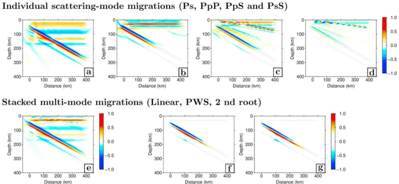
Figure 7. Single-mode migrations of three components receiver function for a 2-D model containing a single interface with 10◦dip and 10%𝛿VP, 𝛿VS, and𝛿𝜌
perturbations (Model WCS2; Table 1). Panel (a) is the PS, (b) the PpP, (c) the PpS, and (d) the PsS migrations (cf. text). The data were generated for 24 sources regularly spaced in back azimuth and with epicentral distances ranging between 30◦and 90◦. The four images recover the structure with the correct polarity but are affected by the other modes. The spurious migrated signals are at different locations in each migration.
patterns into account is key to reducing the contamination of migrated images by the various scattered modes.
Here we demonstrated the importance of the scattering patterns when migrating three component data. Moreover, we showed that integrating the three components of the RF into the imaging principle allows us to coherently retrieve the scattering potential for arbitrarily dipping discontinuities from all back azimuths. 3.3. Multimode Migration
As seen in Figures 5 and 6, free surface multiples are clearly visible in the PS migration, even for very sim-ple settings. They are easily distinguishable in the PS migrated image for this particular model, but their interpretation becomes increasingly more difficult with the complexity of the setting. Here we will show how jointly migrating the four main scattering modes can help mitigate the contamination by free surface multiples in the interpretations of migrated images.
Since free surface multiples tend to be stronger and more difficult to interpret correctly in subhorizontal settings, we choose a model with a 10◦dipping interface, thus placing ourselves in a worst-case scenario situation with regards to free surface multiples (Cheng et al., 2017). In this simulation we use 24 sources to cover all possible back azimuth and incidence angles. The results in Figure 7 show the migrations for the four individual scattering modes for model WCS2 described in Table 1, which has one interface at a 10◦dip. The results for the three-component PS migration are shown in Figure 7a. The dashed line shows the only feature that is present in the synthetic model. We can see a coherent signal that lines up with the structure, but also three spurious features associated with multiples: (1) a negative feature at approximately 180- to 380-km depth that corresponds to the PpP multiple; (2) a positive feature at 250- to 400-km depth that cor-responds to the PpS multiple; and (3) a negative feature between 300- and 400-km depth that corcor-responds to the PsS multiple.
We perform one migration for each scattering mode, and the resulting images can be seen on Figures 7b (PpP), 7c (PpS), and 7d (PsS). We find that the free surface multiples in the synthetic waveforms are correctly migrated in their respective images. However, in each image, three out of the four modes are still visible and wrongly migrated. They appear at different depths and produce spurious structures with different dip angles. Specifically, phases slower than the currently migrated mode are mapped below the true scattering feature (e.g., in Figure 7a), and phases faster than the currently migrated mode are placed above the scattering feature (e.g., in Figure 7d). On these four migrated images, there is overall more spurious features than true features, but their locations are not coherent across the four single-scattering mode migrations. These four images allow us to visually discriminate between real features, which have coherent amplitude across all four images, and the spurious features, which do not correlate on the different single-scattering mode images.
In this example, we can also notice that the time delays are more compressed in the multiple modes, and hence, they have a higher spatial resolution than the direct PS conversion mode, especially for the S scattered waves (Rondenay, 2009). This is due to the fact that a ray covers a single unit distance (upgoing) between two consecutive points in depth for the PS mode and two (downgoing and upgoing) when we migrate a multiple. Here we showed that we are able to migrate the free surface multiples at their correct polarities and positions in depths using the scattering patterns and their respective traveltimes computed with FM3D. Because the
Figure 8. Multimode migrations for a 2-D model containing a single interface with a 10◦dip and 10%𝛿VP, 𝛿VS, and𝛿𝜌perturbations (Model WCS2; Table 1).
(a) Linear stack, (b) phase-weighted stack, and (c) second-root stacks for the multimode migration of the three-component receiver functions with scattering patterns, for 24 sources coming from all azimuths with epicentral distance between 30◦and 90◦.
actual features are always focused at the same depth across all single-scattering mode images, they will sum up positively during the multimode migration. This is something we will exploit in the next section. 3.4. Stacking Methods
We now test the three stacking methods introduced in section 2.7 to see how well they enhance the coherent signals from the four single-scattering mode migrated images in Figure 7. We consider one stacking method with no coherence filter (linear stacking; equation (13)) and two stacking methods that incorporate coher-ence filters—PWS (phase cohercoher-ence filter; equation (16)) and second-root stacking (amplitude cohercoher-ence filter; equation (19)). The results are displayed in Figure 8.
The first method we test is linear stacking (equation (13); Figure 8a), where we simply add the amplitudes of the four modes during the migration with no extra measure of coherence. The resulting amplitudes are then normalized to obtain the final image. Results show that the dipping interface is better imaged than in Figure 7a. We note that the energy from spurious features is considerably reduced but that they do not completely disappear. The three spurious streaks described in Figure 7a are still present just under the actual discontinuity. We also see that there is more noise above the discontinuity than in Figure 7a. In this case, the four modes have comparable amplitudes, and spurious features will only be reduced to about one fourth of their amplitude on a given scattering mode migration.
The second method we test is PWS and corresponds to the imaging principle in equation (16). The results are shown in Figure 8b. The resulting image exhibits fewer artifacts than with the linear stack, as most spurious signals do not have a coherent phase over the four modes. The phase stack virtually acts as a filter applied to the linear amplitude stack, as the artifacts are at the same position in depth, but their amplitude is even more reduced, representing less than 10% of their single-mode values.
Finally, the last method we test is second-root stacking and corresponds to the imaging principle in equation (19). The results are shown in Figure 8c. The image is very similar to Figure 8b and has all the artifacts reduced to less than 10% of the actual discontinuity.
The test conducted in this section demonstrate that most artifacts can be eliminated by applying coherence filters based either on phase (phase-weighted stack) or amplitude (second-root stack) in simple synthetic cases. We are now going to test these methods with a more complex synthetic model depicting an idealized subduction zone.
3.5. The 2.5-D Subduction Zone
Here we show how our imaging principle can be used to improve interpretations in realistic settings. To do so, we design a synthetic subduction zone model, labeled R2DSZ in Table 1, and analyze the migrated images obtained using equations (12), (13), (16), and (19). In this model, we have four different layers over a half-space with constant elastic properties and use a total of 24 sources equally spaced in back azimuth with random epicentral distance to the center of the array ranging between 30 and 90◦. The array starts at lateral position 0 km and covers 400 km in length.
The results for the four single-mode migrations are shown in Figures 9a to 9d. Figure 9a shows the migration of the forward PS scattering mode. The single-mode migration is able to resolve the overriding Moho and the