HAL Id: hal-00302866
https://hal.archives-ouvertes.fr/hal-00302866
Submitted on 18 Jun 2007
HAL is a multi-disciplinary open access
archive for the deposit and dissemination of
sci-entific research documents, whether they are
pub-lished or not. The documents may come from
teaching and research institutions in France or
abroad, or from public or private research centers.
L’archive ouverte pluridisciplinaire HAL, est
destinée au dépôt et à la diffusion de documents
scientifiques de niveau recherche, publiés ou non,
émanant des établissements d’enseignement et de
recherche français ou étrangers, des laboratoires
publics ou privés.
methods in space, Fourier frequency, and eigen domains
Qiuming Cheng
To cite this version:
Qiuming Cheng. Multifractal imaging filtering and decomposition methods in space, Fourier frequency,
and eigen domains. Nonlinear Processes in Geophysics, European Geosciences Union (EGU), 2007,
14 (3), pp.293-303. �hal-00302866�
www.nonlin-processes-geophys.net/14/293/2007/ © Author(s) 2007. This work is licensed
under a Creative Commons License.
Nonlinear Processes
in Geophysics
Multifractal imaging filtering and decomposition methods in space,
Fourier frequency, and eigen domains
Qiuming Cheng
State Key Laboratory of Geological Processes and Mineral Resources, China University of Geosciences, Wuhan 430074, Beijing 100083, China
Department of Earth and Space Science and Engineering, Department of Geography, York University, Toronto M3J1P3, Canada
Received: 14 February 2007 – Revised: 23 April 2007 – Accepted: 29 May 2007 – Published: 18 June 2007
Abstract. The patterns shown on two-dimensional images
(fields) used in geosciences reflect the end products of geo-processes that occurred on the surface and in the subsurface of the Earth. Anisotropy of these types of patterns can pro-vide information useful for interpretation of geo-processes and identification of features in the mapped area. Quantifica-tion of the anisotropy property is therefore essential for im-age processing and interpretation. This paper introduces sev-eral techniques newly developed on the basis of multifractal modeling in space, Fourier frequency, and eigen domains, respectively. A singularity analysis method implemented in the space domain can be used to quantify the intensity and anisotropy of local singularities. The second method, called S-A, characterizes the generalized scale invariance property of a field in the Fourier frequency domain. The third method characterizes the field using a power-law model on the basis of eigenvalues and eigenvectors of the field. The applications of these methods are demonstrated with a case study of Envi-ronment Scan Electric Microscope (ESEM) microimages for identification of sphalerite (ZnS) ore minerals from the Jind-ing Pb/Zn/Ag mineral deposit in Shangjiang District, Yunnan Province, China.
1 Introduction
Fractal models are often used to characterize self-similar ge-ometries, whereas multifractal models have been utilized to quantify patterns (fields) defined on sets which themselves can be fractals. Extension from geometry to field has sig-nificantly increased the applicability of fractal/multifractal theories and methods. For example, for processing and an-alyzing complex images for pattern recognition and spatial information extraction can be assisted with methods related
Correspondence to: Qiuming Cheng
to the multifractal theory. Owing to multiple moment func-tions involved in defining partition funcfunc-tions, the multifractal models are capable of characterizing the entire variance of the fields, which makes multifractal models unique in com-parison with other low-order moment statistics that can only characterize the variance of majority values of the field but usually are not capable of characterizing the variability of singular values because of their rarity. However, singular val-ues in a field are often of special interest in the geosciences. For example, most hazardous geological processes yield sin-gular value distributions, such as floods, which produce ex-treme flow events (Malamud et al., 1996). Earthquakes cause extreme energy release (Turcotte, 1997), and landslides can cause loss of mass in land areas (Malamud et al., 2004). Other types of singular processes include cloud formation (Schertzer and Lovejoy, 1987), rainfall (Veneziano, 2002), and hurricanes (Sornette, 2004). These types of non-linear natural processes often cause hazardous problems to human beings. Mineralization can cause concentrations of elements in rocks that can be mined as ores. It is essential to deal with these types of singularity that are involved in the singu-lar processes. It has been proved that multifractal modeling is an effective means for characterizing singular patterns ob-served in a field.
Since the concepts underlying the multifractals were orig-inally introduced by Mandelbrot (1972, 1974) in the discus-sion of turbulence (Feder, 1988), various multifractal models have been developed, and some of these have been widely used in various fields of science for characterizing measures with scaling properties (Frisch and Parisi, 1985; Grassberger, 1983; Hentschel and Procaccia, 1983; Badii and Politi, 1984, 1985; Halsey et al., 1986; Schertzer and Lovejoy, 1991; Ev-ertsz and Mandelbrot, 1992; Agterberg, 1995, 2005, 2007; Cheng, 1997, 1999a). Several multifractal models have been used in geoscience to analyze maps or patterns observed on the surface or near the surface of the Earth or remotely sensed from space. A large number of papers published in
the literature have indicated that study of multifractals and multifractal modeling has been one of the focuses in non-linear geoscience. These models include the box-counting-based moment method (Halsey et al., 1986), the histogram-based model (Paladin and Vulpiani, 1987), the double-trace moment method (Schertzer and Lovejoy, 1991), the multi-plier method (Chhabra and Sreenivasan, 1991), the wavelet method (Beery et al., 1990, cited in Schertzer and Lovejoy, 1991), and the gliding-box-based moment method (Cheng, 1999a).
Among these models, the box-counting-based moment method has been commonly used to analyze one-dimensional (1-D) or two-dimensional (2-D) values for measures or fields. The box-counting moment method involves se-quential partitioning of the study area (2-D field or sup-port) and upscaling processes to form measures µ(ε) at variable scales ε. It uses three functions: mass exponents τ (q)= limε→0LogPµq(ε)/Logε a
singular-ity index α(q)=∂τ (q)∂q , and a fractal dimension spectrum
f (α)=α(q)q−τ (q). These three functions are related through Legendre transformation. In a case in whichPµ(ε)
is constant, independent of the partition scale εgnd imply-ing that the total measure at all scales remains unchanged, then the measure is called conservative, in which τ (1)=0. Otherwise, if the total measurePµ(ε) changes according
to a power law with the scale ε, implying a sort of gain-ing or losgain-ing measure as the partitiongain-ing processes proceed, then τ (1)6=0, which corresponds to a non-conservative situ-ation. It characterizes the overall heterogeneity of the field by means of singularity analysis. Since the partition usually involves regular grids of variable sizes, the moment-based multifractal models can only characterize the isotropic scale invariance property of the measure.
A more general anisotropic scale invariance property can be characterized in the Fourier domain. For example, a gen-eralized scale invariance (GSI) paradigm was developed by Schertzer and Lovejoy (1991) using the power spectrum den-sity function. A spectrum and area model (S-A model) was developed for quantifying the anisotropic scaling invariance property in the Fourier domain that yields a new filtering technique for decomposition of mixing patterns on the basis of a new fractal distribution of the power-spectrum density (Cheng et al., 1999; Cheng, 2004).
A similar method, called MSVD, for unmixing spatial pat-terns was developed by Li and Cheng (2004) on the basis of eigenvalues and eigenvectors calculated from a map treated as an asymmetrical matrix. Cheng (2005) proved that the ab-solute values of eigenvalues and eigenvectors calculated from a map generated by multiplicative cascade processes follow non-conservative multifractal distributions, and the number of large eigenvalues follow the power-law frequency distri-bution (the N-λ method) (Cheng, 2005).
These types of power-law models – including the C-A method in the space domain (Cheng et al., 1994), the S-A
method in the frequency domain (Cheng et al., 1999, 2001), and the N-λ method in the eigen domain – can be utilized for defining breaks to separate patterns with distinct general-ized self-similarities. In using the C-A method the values of a field can be directly separated into components that reflect anomalous and background values. With the S-A method the power spectrum density field can be separated into com-ponents with distinct self-similarities that can be converted back to the space domain to correspond to decomposed pat-terns with distinct generalized self-similarities. In applying the N-λ method the eigenvalues, and accordingly the eigen-vectors calculated from a field, can be classified into groups on the basis of self-similarity so that these groups can be con-verted back to the space domain to form unmixed patterns.
This paper is organized first, to introduce the principle of the methods of local singularity analysis (α-method), the spectrum-area (S-A) method, and the large eigenvalues-based method (N-λ). Then a case study of analyzing ESEM microimages for the identification of sphalerite (ZnS) ore minerals from a Pb/Zn/Ag mineral deposit in Shangjiang District, Yunnan Province, China, was used to demonstrate the applications of these methods.
2 Mapping local singularity in the space domain
From the multifractal theory we can prove that the extreme density values along the two tails may follow power-law fquency distributions, which can be expressed as the C-A re-lationship, A(≥C)∝C−β, where A is the area with density (concentration) values above a cutoff value C, and β is a positive value (Cheng et al., 1994). Area A can be in an irregular shape, depending upon the anisotropic property of the density values. Given the scaling property of the multi-fractal measures, if one restricts the area to a small area, or as a pixel scale the C-A model can be replaced by a local
α-value model to be introduced in detail in this section.
As-sume that for a given small area (A), centered at a location on the map, where A is the area in a mineralization domain or mineralization-influenced space, denotes the amount of metal contained in the domain (A) as µ((A)). The metal concentration in the same area (A) can be expressed as
ρ((A))=µ((A))/A. When the size A changes, the
quanti-ties µ((A)) and ρ((A)) change accordingly. For example, when size A decreases, the value of the metal µ((A)) de-creases. However, the quantity ρ((A)) will vary, depending on the properties of metal distribution in the small area A.
From a mulifractal point of view, these quantities µ((A)) and ρ((A)) follow power-law relationships with the area A as
µ[((A)] = cAα/2 (1)
ρ[((A)] = cAα/2−1 (2) where µ((A)) is the total amount of metal in (A), and
first law model (1), α is the exponent of the power-law relationship. The power-power-law function is completely de-termined by the two parameters c and α. The first parameter (c) determines the magnitude of the function, whereas the second parameter (α) determines the shape of the function or the changing behavior of the quantity with the change of A. The shape of (A) can be a simple geometric form such as a circle, rectangle, or square, corresponding to isotropic scaling. The shape can also be more complex, correspond-ing to anisotropic scalcorrespond-ing (Cheng, 2004). If α is constant across the entire image, then the spatial patterns follow a monofractal distribution; otherwise, if α has multiple finite values, then the spatial patterns may follow a multifractal distribution (Cheng, 1999b). The exponent (α) is termed the singularity index, which determines the distribution of the degree of singularity of the field. It characterizes how the statistical behavior of metals in area (A) varies as A (mea-suring scale) decreases. Although theoretically the power-law relationships (1) and (2) hold true for a large range of A (for example, a few orders of magnitude of scale), the actual range of scaling is usually limited to a finite range of A ow-ing to the limitation of the data resolution. The values of the exponent α can be grouped into two categories: In some lo-cations ρ((A)) is independent of the size A, implying α=2; in other locations ρ((A)) may, however, depend on the size of A, implying α6=2. The former case is considered as non-singular, but the latter as singular. If A becomes very small at a singular location, then ρ((A)) either approaches zero or infinity. We differentiate further between positive singu-larity α<2 and negative singusingu-larity α>2. The mean value
ρ((A)) calculated at a given location with positive
singu-larity increases with reduced area size A, whereas ρ((A)) at another location with negative singularity decreases as the area size A decreases. The index α can be estimated from the values ρ((A)) calculated at different sizes of A by means of least squares .The singularity index has the following prop-erties (Cheng, 1999b): α=2, if and only if ρ((A)) equals a constant, independent of size A; α<2 if and only if ρ((A)) is a decreasing function of A, which implies a “convex” prop-erty of ρ((A)) around the given location; and α>2 if and only if ρ((A)) is an increasing function of A, which indi-cates a “concave” property of ρ((A)) around the given loca-tion. The former case indicates that metal concentration at a location with positive singularity may be enriched, and at the location with negative singularity it may be depleted. Min-eralization generally corresponds to ore bodies with metal concentration enrichment. The α-values can be mapped and compared with the locations of known mineral deposits.
Two methods can be applied to estimate the α-values: the regular windows-based method and contour-based meth-ods (Cheng, 2006). In the windows-based method, for a given location on the map, a set of sliding windows A(r) (squares, circles, and rectangles) with variable window sizes,
rmin=r1<r2<. . . <rn=rmaxare chosen to calculate the aver-age concentration value ρ[A(ri)]. These ρ[A(ri)] values
(i=1, . . . , n) will show a linear trend with a linear size ri on
log-log paper, or Logρ[A(r)]=c+(α−2)Log(r). The slope es-timated from the linear relationship can be considered as the estimate of α−2. A similar treatment with sliding windows at all locations on the map can create a singularity distribu-tion map. The uncertainty related to the estimadistribu-tion of the singularity index also can be recorded and mapped. Only singularities with relatively small uncertainty will be further considered. The scale range [rmin, rmax] can be determined by observing scaling properties of the power-law functions and consideration of the scales of the local structures of in-terest. The left bound rminis often limited by the resolution of the data. Different ranges of [rmin, rmax] to be used in ensuring distinct power-law functions may yield singulari-ties at different scales; for example, small-scale singularity may reflect local anomalies associated with mineralization, whereas large-scale singularity may represent regional back-ground variability. In the contour method, the windows (A) is replaced by closed contour lines, and the value ρ[(A)] by the average value of the entire area enclosed by the contour. The shapes of the contours are determined by the actual data around the location.
The singularity index calculated from 2-D maps usually has values around 2. The areas with non-singular values (α=2) generally occupy most parts of the map with a di-mension close to 2 (a box-counting didi-mension). In these ar-eas the element concentration may show normal variability so that the average concentration calculated within the win-dows (A(r)) is close to a constant and independent of the windows size r. The other areas with singular values (α6=2) occupy a relatively small part of the map, with dimensions
<2. From a statistical point of view, a majority of values
on the geochemical map with α≈2 follow either normal or lognormal distributions, whereas a minority of values (ex-tremely high and low values along both frequency distribu-tion tails) on the map with a singularity of α6=2 may follow Pareto distributions. Separating the extreme-value distribu-tions from normal and lognormal distribudistribu-tions is essential for anomaly identification. Most ordinary statistics that require the assumption of normal or lognormal distributions of sam-ple values may not be effective in dealing with these types of singularity distribution.
It should be pointed out that the above discussion is based on an assumption that the window A is a small area but never be as small as a point in reality due to data resolution. This is important because for the multifractals generated by stochastic process for example random multiplicative cas-cade they have no pointwise convergence properties of sin-gularity. They have only the weak convergence property that integrals over finite sets may converge. In this sense, the mul-tifractal itself cannot be specified at a mathematical point. Therefore, the localized singularity concept introduced in the current paper is different from conventional pointwise sin-gularity defined in mathematical function. From geostatis-tics point of view, a mapped distribution of measures can
be considered as realization of the stochastic cascade pro-cesses and the singularity becomes regionalized random vari-able and the estimated values becomes the realization of the random variable. The average value of many realizations will be the expectation of the singularity. In reality there are of-ten only one set of measurement (a map) which should be considered as only one realization.
3 Anisotropic scaling modeling in the Fourier fre-quency domain
Fourier/inverse Fourier transformation has been commonly used for time series analysis and signal processing. Spec-tral energy density functions characterize the power spectrum distribution in the frequency domain. The advantage of deal-ing with fields in the frequency domain is that some complex convolution operations in the spatial domain for correlation analysis, filtering, and transformation can be simplified sig-nificantly in the frequency domain. Moreover, anisotropic spatial distribution of a spectral energy density retains the spatial structure of a field. Therefore, spatial analysis can be applied to anisotropic spectral energy density in the fre-quency domain to construct filtering functions to process the field (Cheng, 2001a, b; Cheng et al., 1999, 2001). Schertzer and Lovejoy (1991) developed the concept of general scale invariance (GSI). In the formulism of GSI, taking the 2-D problem as an example, the scaling in the x and y directions will not be at the same scale-changing rate. Similarly, follow-ing the linear GSI formulism, it associates the measure and the measuring scale with a scale transformation Tλ=λ−G,
where G is a 2×2 matrix (for the 2-D problem) and λ is a scale ratio. If G=I as the unity matrix, then the transforma-tion becomes the isotropic transformatransforma-tion. Otherwise, if G is not unity, then the transformation characterizes anisotropic scale invariance (Schertzer and Lovejoy, 1991). In the scale-changing operator, it involves four parameters: d is a mea-sure of overall contraction, c is a meamea-sure of the relative scaling of the two coordinate axes, f represents reflection across a line diagonal to the axes, and e is a measure of ro-tation. Schertzer and Lovejoy (1991) demonstrated that the spectral-energy density of a field with the generalized scal-ing invariance property under the formalism of GSI can be expressed as
< S( ˜Tλω) >= λ−s < S(ω) > (3)
where S represents spectral-energy density, ω is a wave number, ˜Tλ=λG˜ is the scale-changing operator in Fourier
space, ˜G is the generator in Fourier space, λ is scale ratio,
and s>0 is the exponent. In the case of linear GSI, ˜G=GT, the transposition of the real space generator. Schertzer and Lovejoy’s work can characterize the general scaling property of multifractal measure in Fourier domain by estimating the scale transformation. Various techniques have been devel-oped for quantifying the anisotropic scale invariance under
the formalism of GSI. The scale invariance generator (SIG) is one iterative technique developed for estimating the transfor-mation operator G and for calculating the generalized scal-ing exponent s of model (3) (Lewis et al., 1999). The unique significance of the GSI concept and techniques is its capa-bility for modeling the general scale transformation and the scaling exponent. One challenge of using this iterative SIG technique is its convergence speed and the sensitivity of the estimates.
Cheng et al. (1999) proposed a new S-A model to rep-resent the law frequency distribution of the power-spectrum density. A new function relating the multifractal model and the spectral-energy-density function was derived (Cheng, 2004) to show the power-law relationship between the spectral-energy-density value (S) and the “area” of the set (≥S) with spectral-energy-density values above S on the power-density plane,
A[(≥ S)] ∝ S−2d/s (4) where 2d is related to the so-called elliptical dimension with
d=1, corresponding to isotropic dimension, and s>0, the
ex-ponent of the power law. Model (4) can be implemented us-ing contours determined by the data on the plane of power density, and the contours can be in any self-similar geome-try that characterizes the general scale transformation. The estimate of s is the general scaling exponent. The disad-vantage of model (4) in comparison with model (3) is that it does not give the explicit scale transformation, but the ad-vantage might be its quick estimation of the general scaling exponent. An integration of these two methods was explored by Chao and Cheng (2005) to use the estimation of s from model (4) as the “best” initial value for conducting the it-erative SIG. It has been shown that the result estimated for s from model (4) is often the final estimation of the iterative SIG method. In a later section of this paper, it will be demon-strated that model (4) can be used for image filtering and map decomposition. The assistance of SIG can also provide fur-ther information about the details of anisotropy properties of the decomposed field components.
4 Anisotropic scaling modeling in the eigen domain
To consider a map as a large matrix, one can use linear al-gebra to process the map. Eigenvalues and Eigenvectors can be used to decompose the matrix. Here we introduce the result obtained for large matrices generated by multiplica-tive cascade processes and that can be modeled as multifrac-tals. It has been proved (Cheng, 2005) that the eigenvalues of anisotropic deterministic multiplicative cascade multifrac-tal measures describe a multifracmultifrac-tal distribution that char-acterizes the orientational heterogeneity, whereas the ordi-nary multifractal model of the measure itself characterizes the overall heterogeneity. Therefore, calculating the multi-fractal distribution of eigenvalues of a 2-D field in addition
to the multifractal distribution of the field itself may pro-vide supplementary information about the heterogeneity of the field. Although the discussions were for multifractal dis-tributions of eigenvalues and eigenvectors of a 2-D field gen-erated from deterministic multiplicative cascade processes, the results may have a general implication for other types of 2-D multifractal fields. It is therefore possible to form a new model to characterize a 2-D field by its eigenvalues and eigenvectors from a multifractal point of view. This study has provided a framework for implementing multifractal model-ing in the eigen domain, which has a number of advantages as previously mentioned.
This result is also useful for exploring the distribution of large eigenvalues from a 2-D matrix. Large eigenval-ues are often of interest in most principal component anal-yses because they carry a substantial part of the data vari-ance. According to the C-A model derived by Cheng, Agter-berg, and Ballantyne (1994), the distribution of the extremely large eigenvalues under the current discussion may follow the power-law distribution
N (≥ λ) ∝ λ−β (5)
where λ stands for eigenvalue and β is the exponent of the power-law relationship. The significance of model (5) is not only because it establishes a power-law frequency-distribution model of large eigenvalues but also gives an ex-ample of characterizing a compete distribution of extreme values from a multifractal distribution. The study of extreme value distribution has been a subject of interest not only in statistics but also in many applied fields. The common dif-ficulty for approximating extreme value distribution is due to lack of enough data (samples) to show the complete be-havior of extreme values or events. Consequently, there has rarely been seen a complete distribution of extreme values from a multifractal distribution with high level of confidence (Cheng, 2006). Although the result of model (5) was proved true for multifractal fields generated by deterministic multi-plicative cascade processes the model has been tested with a large number of images including aeromagnetic field from various places, cloud photos, DEM, geochemical concentra-tion in water, stream and lake sediments. These results are not shown in the paper.
5 Decomposition of multifractal measures
Scaling characterization in the geosciences is a growing field in the nonlinear geosciences. Utilization of fractal and mul-tifractal modeling for the conventional tasks of classification in the geosciences has also become a potential field for in-novative scaling analysis. This section introduces several ex-amples of using power-law models for image filtering and pattern decomposition.
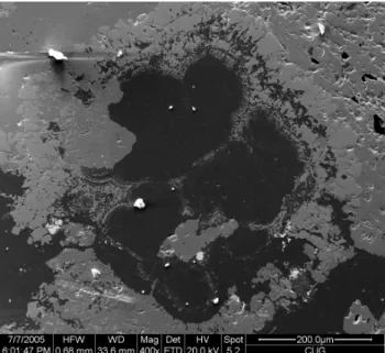
Figure 1. Microscope image of a sphalerite ore sample collected from Jinding lead Fig. 1. Microscope image of a sphalerite ore sample collected from
Jinding lead and zinc mineral deposit, Yunnna, China.
5.1 Local singularity analysis for high-pass filtering From model (1) we can express the local singularity index
α-value as the following expression:
α=2log µ[(A1)]− log µ[ (A2)]
log A1− log A2
=dµ[ (A)] dA
2
ρ[ (A)] (6)
The above expression (6) involves the first derivative of the measure over the area of the measuring scale, which im-plies that the α-values can be considered a type of high-pass filtered results having unique characteristics in comparison with other types of high-pass filters – for example, the α-value is independent of scale A, although the expression in-cludes the term A. In practice, this is very important, because the filtering results are independent of the window sizes up to the threshold within which the scaling properties (1) and (2) hold true. Choosing specific forms of the shape of area A can yield different anisotropic high-pass-filtering methods. The method with square windows of A is demonstrated by the case study in this paper.
5.2 S-A method for pattern decomposition in the frequency domain
As discussed previously, filtering in the frequency domain with Fourier/inverse Fourier transformations has been com-mon in many fields of the geosciences. The main advan-tage of conducting filtering in the frequency domain is be-cause the properties of complex convolution operations in the space domain used for filtering can be simplified as normal
(a)
(c) (b)
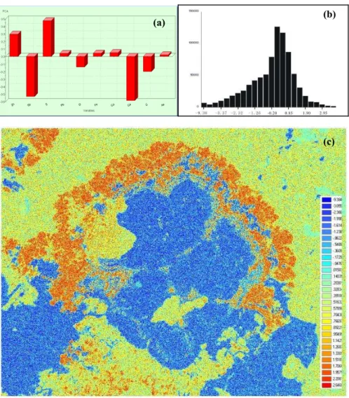
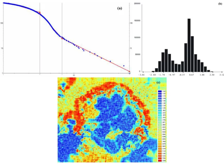
Fig. 2. Results obtained using principal component analysis (PCA) applied to ESEM images of elements Zn, Sb, S, Pb, O, Fe, Cu, Ca, C and
As scanned using ESEM facility provides by the State Key Laboratory of Geological Processes and Mineral Resources, China University of Geosciences. The ESEM images have 1024×800 pixels. (a) Plot showing loadings of elements on the first principal component calculated using GeoDAS GIS software. Inputs are ESEM images and correlation coefficient model was used for PCA. The result shows first com-ponent is positively correlated with sphalerite (ZnS) and negatively associated with CaCO3 and Sb; (b) a histogram showing the frequency distribution of scores of ESEM images on the first component; and (c) an image showing the distribution of scores of ESEM images on the first component. Blue patterns represent calcites (CaCO3) and orange patterns show splarelite (ZnS). The same classification using standard deviation scheme was used for both the image (c) and the histogram (b).
products of Fourier transformed functions in the frequency domain, as expressed below:
F [µ ⊗ g] = F [µ] F [g] (7) where F [] stands for Fourier transformation, and ⊗ for the convolution operation applied to functions µ and g. It has been found that the power-law relationship (3) can often be fitted with several straight-line segments on a log-log-scale plot. Each range of spectral energy density within which re-lation (3) holds true can be used to define a filter. For ex-ample, if two straight-line segments are fitted to the data, and these straight lines yield the threshold S0, then two fil-ters can be defined as F [gB(ω)]=1 if S(ω)>S0, and
other-wise F [gB(ω)]=0; and the second filter as F[gA(ω)] = 1 if
S(ω) ≤S0, and otherwise F [gA(ω)]=0. From the definition
of F [gA(ω)] and F [gB(ω)], we can see that the shapes of
the filters could be irregular, depending on the complexity of the spectral-energy-density distribution. However, in gen-eral, the wave numbers ω in filter F [gA(ω)] are relatively
larger than those in F [gB(ω)], implying that the frequency
in F [gA(ω)] is relatively higher than that in F [gB(ω)]. In
this sense, gA corresponds to a relatively high-pass filter,
and gB to a relatively low-pass filter. However, one must
keep in mind that the two filters are not sharply bounded ei-ther by frequency or by wave numbers. They are defined in such a way that the spectral-energy-density distributions of
the two filters satisfy distinct power laws or have different anisotropic scaling properties. Applying the inverse Fourier transformation, with these two filters applied to the Fourier transformed functions, we get decomposed components in the space domain:
µA= µ ⊗ gA= F−1{F [µ] F [gA]}
µB= µ ⊗ gB= F−1{F [µ] F [gB]} (8)
where F−1stands for inverse Fourier transformations. The two components µB and µAhave different frequency
prop-erties quantified by two distinct power laws in the frequency domain.
5.3 N-λ method for pattern decomposition in the eigen do-main
If a map is treated as a matrix M(µ), it can be decomposed into products of eigenvalues and eigenvectors
M =
n
X
i=1
λiPiQTi (9)
where λi stands for the non-zero eigenvalues
(|λ1|≥|λ2|≥. . . ≥|λn|>0) and Pi and Qi for the left
and right eigenvectors, respectively. Because the matrix M is usually not symmetrical, the eigenvalues could be imaginary values. In his Ph.D dissertation, Li (2004) proposed a power-law model for associating the accumulation of sorted eigenvalues and the cutoff value of the eigenvalues as
k
X
i=1
λi ∝ λβk. (10)
On the basis of the above model, an MSVD method was proposed and applied for decomposing map patterns (Li and Cheng, 2005). A computer program was also prepared by Li (2004) to calculate the eigenvalues and eigenvectors. From multiplicative cascade processes and multifractal the-ory, Cheng (2005) proved that model (4) holds true for mul-tiplicative cascade multifractal distributions. Thus model (4) should be used for defining breaks to separate eigenvalues into groups, and then each of the groups can be combined to form decomposed components of the map.
6 Filtering ESEM images of sphalerite ore samples from the Jinding deposit, Yunnan, China
The data set chosen for method validations and applications is the analysis of ESEM microimages from ore samples col-lected from the Jinding Pb/Zn/Ag mineral deposit, in the northern part of the Lanping-Simao Basin, Yunnan Province, China. This deposit is the largest Pb/Zn/Ag deposit in China, with reserves of about 200 Mt of ore, grading 6.08% Zn and 1.29% Pb. Because it is hosted in Cretaceous and Tertiary
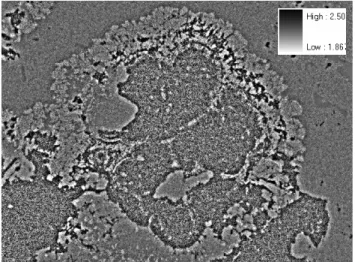
Figure 3. An image showing distribution of local singularity calculated using
ε
α α
α ≈
Fig. 3. An image showing distribution of local singularity
calcu-lated using GeoDAS from the scores of ESEM images on the first component (Fig. 2c). To avoid negative value of the image, a con-stant value 10 was added to the image Fig. 1c prior to the calcula-tion of singularity index. Square windows with sizes ε=1, 3, . . . , 61 pixel units were used for the multiscale calculation. The light areas correspond to α<2, dark areas with α>2 and grey areas with α≈2.
terrestrial rocks controlled by a complex dome structure, the genesis of the deposit has been debated, mainly between a syngenetic formation and an epigenetic formation (Xue et al., 2006). Evidence in support of model generalization has been sought by geologists from studies of mineralogy, iso-topes, geochemistry, structure, and tectonics. The objective of the case study in this paper is to process the mineral mi-croimages taken under ESEM using the new techniques in-troduced in the paper. In the summer of 2004 a large num-ber of ore samples were collected from the Jinding deposit by the author’s research group for systematic study of min-eral textures from a non-linear process point of view. Sev-eral analyses have been made from these samples, including microimages captured using ESEM, trace element chemi-cal concentrations by inductively-coupled-plasma mass spec-troscopy (ICP-MS), and mineral identifications by electron probe. This study used ESEM images as an example to demonstrate the application of the image-processing tech-niques. Figure 1 shows a microscopic image of an ore sample taken under electron microscopy at 400× magnification by the State Key Laboratory of Geological Processes and Min-eral Resources, China. On the image, dark color patterns represent calcite (CaCO3), and light gray patterns with pos-itive relief represent sphalerite (ZnS), with the outer part be-ing unknown. The sphalerite patterns show a hexagon form, which may indicate that the sphalerite formed by altering and replacing calcite along the edge of the calcite grain, and that the thin section is cut perpendicular to the c-optical axis of the calcite. To map the distribution of minerals in the sample, several images were scanned using ESEM for the elements
(a)
(b)
(c)
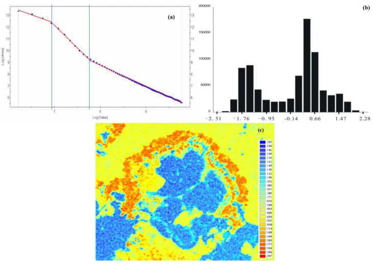
Figure 4. Results obtained using S-A filtering method (see text for details). (A) Plot
Fig. 4. Results obtained using S-A filtering method (see text for details). (a) Plot showing the relationship between power spectrum density
labeled as log (value) and the area with power spectrum density above a threshold labeled as log area. Log-transformation is natural log. Three straight-line segments were fitted to the data by means of least squares. These three straight-line segments show different slopes and yield two breaks of power spectrum density values. The first break from the right was used as cutoff value for filtering the original image Fig. 2c with a low-pass filter. The results are shown in (c) and the frequency distribution of the filtered image is shown in (b). Blue patterns represent calcites (CaCO3) and orange patterns show sphalerite (ZnS). The same classification using standard deviation scheme was used for both the image (c) and the histogram (b). The histogram (b) clearly shows two populations one for calcites (CaCO3) and the other for sphalerite (ZnS).
As, Bi, C, Ca, Cd, Cr, Cu, Fe, O, Pb, S, Sb, Se, Sr, Ti, and Zn. Each image has 1024×800 pixels and is about 3 MB in size. Some images – for example, Bi, Cd, Cr, Pb, Se, Sr, and Ti – do not show significant variation. Other images of the ele-ments As, C, Ca, Cu, Fe, O, S, Sb, and Zn, with good quality, were processed using a principal component analysis (PCA) method for characterizing element associations. It was im-plemented using GeoDAS GIS software (Cheng, 2000) with a correlation coefficient model. The loadings of the first cipal component shown in Fig. 2a indicate that the first prin-cipal component is dominated by the elements Zn and S pos-itively and by Sb, Ca, C, and O negatively. Therefore, the first component mainly represents the sphalerite (ZnS; pos-itive correlation) and calcite (CaCO3; negative correlation). The scores of elements of the first component are shown as both frequency distributions in Fig. 2b and spatial
distribu-tions in Fig. 2c. From the histogram (Fig. 2b) we can see that the values of scores follow a skewed distribution with-out a clear separation of sphalerite and calcite, although on the map in Fig. 2c these two types of minerals generally show distinct patterns – for example, the former in orange and the latter in blue.
In order to filter the image to enhance the patterns of spha-lerite and calcite, the three methods discussed in the previous sections were applied to the image in Fig. 2c. First, the local singularity analysis method was applied to the image for a high-pass filtering of the image. Because the image has neg-ative values, a small constant value of 10 was added to the image to raise all values to be positive. Thus a constant value added to the entire map should not change the local variabil-ity of the map. It may affect the actual estimation of the sin-gularity of the map. For example, the relationships in Eqs. (1)
(a)
(b)
Figure 5. Results obtained using N-λ model (see text for details). (A) Plot showing the
λ λ
(c)
Fig. 5. Results obtained using N-λ model (see text for details). (a) Plot showing the power-law relationship between the number of
eigenvalues (N[>|λ|]) and absolute value (|λ|) of eigenvalue. Log-transformation is natural log. A straight-line segment was fitted to the first 26 large eigenvalues by means of least squares. This straight-line segment determines a break of eigenvalue separating the eigenvalues into two groups: one group with absolute eigenvalue smaller than the 26th eigenvalue and the other group with eigenvalues larger than or equal to the 26th eigenvalue. The latter was further combined with their corresponding eigenvectors to form a map in (c). The frequency distribution of the image is shown in (b). Similarly, blue patterns represent calcites (CaCO3) and orange patterns show sphalerite (ZnS). The same classification using standard deviation scheme was used for both the image (c) and the histogram (b). The histogram (b) clearly shows two populations one for calcites (CaCO3) and the other for sphalerite (ZnS).
and (2) will approximately be power-laws when the box is very small. In this case the effect on the estimation of sin-gularity index will be minimized. Otherwise one can apply the singularity analysis to individual ESEM images which have positive values only. For this example, the singularity highlights the edges of the minerals and the small variance related to the actual values of singularity won’t significantly change the result. Squares of multiple sizes – for example, a half size ranging from 1 to 30 pixels-were utilized to calcu-late the singularity index α values; the results are shown in Fig. 3. The filtered map (Fig. 3) clearly enhances the outlines of sphalerite with white and black patterns, corresponding to lower and higher values of α, respectively. The S-A method was also applied to the image (Fig. 2c). First, the image was converted into the Fourier domain by Fourier transformation,
implemented in GeoDAS, and then the values of the power-spectrum density were fitted with straight-line segments by means of least squares according to model (4). The results are shown in Fig. 4a. The data were fitted with three straight-line segments by means of least squares. Two breaks of power-spectrum-density values, 1029.94 and 2343.29, were identified, separating the power-spectrum-density values into three ranges: <1029.94, 1029.94–2343.29, and >2343.29, respectively. The slopes of the three straight lines from the right are −1.788, −3.836, and −1.385, respectively. The first break from the right, 2343.29, was used as the cutoff value to form a binary filter, eliminating the high-frequency com-ponent of the image that corresponds to the wave numbers, yielding a power-spectrum density >2343.29.
The filtered results are shown both as a histogram in Fig. 4b and a map in Fig. 4c, respectively. The former clearly shows two populations, one for sphalerite and the other for calcite, and the latter shows sphalerite and calcite reflected as orange and blue patterns, respectively. Similarly, N-λ was applied to the image (Fig. 2c), and the frequency distribu-tion of eigenvalues is shown in Fig. 5a. The first 26 largest eigenvalues were fitted with a straight line by least squares, which yields a slope of −2.9 and an intercept of 4.1. These 26 largest eigenvalues and their corresponding eigenvectors were used to construct a map according to model (8), and the results are shown in Figs. 5b and c. The histogram shows two separate populations of sphalerite and calcite, and the filtered map shows these two types of minerals in different colors.
The applications of the three new methods to the min-eral image have enhanced the image both as map patterns and frequency distributions of image values. The outlines of sphalerite highlighted on the images in Figs. 3, 4c, and 5c indicate that the outer outlines of sphalerite are relatively reg-ular, in hexagon form, than the inner outlines, in ring shapes. This may indicate an inwardly growing process whereby sphalerite replaces calcite gradually from the edge of the cal-cite inward. This result may provide insights in understand-ing the genesis of the deposit.
7 Conclusions
Among the three new power-law models introduced for char-acterizing scaling properties of multifractal fields as 2-D maps, the local singularity model quantifies the local scal-ing property of the 2-D map in the space domain, and it can be used as a pass-filter technique to enhance high-frequency patterns usually regarded as anomalies when ap-plied to 2-D maps. The S-A model has been shown to be a general model for quantification of the scaling property (anisotropy) of 2-D maps in the frequency domain. This model can be used to construct irregular filters in the fre-quency domain according to the distinct, self-similar dis-tribution of the power-spectrum density value. The N-λ model characterizes a power-law frequency distribution of large eigenvalues calculated from 2-D maps treated as matri-ces. This model can be used to identify eigenvalue groups on the basis of power-law frequency distribution. It was demon-strated that this model is effective for decomposing 2-D maps by selecting groups of eigenvalues and corresponding eigen-vectors. The results obtained by applying these three meth-ods to the mineral microimages collected from the Jinding Pb/Zn/Ag deposit have demonstrated that the three models are generally valid for characterizing 2-D images and that the filtering methods developed on the basis of these power-law models are effective for filtering images.
Acknowledgements. The author thanks graduate students Z. Wang
and Z. Chen for preparing the raw images and data for this study. Thanks are due to two reviewers for their constructive comments.
The research was jointly supported by NSERC Discovery Research Grant (ERC-OGP0183993), a Distinguished Young Researcher Grant (40525009), a Strategic Research Grant (40638041) awarded by the Natural Foundation of Science of China and a 863 High Tech program (2006AA06Z115) by the Ministry of Science and Technology of China.
Edited by: A. Tarquis
Reviewed by: A. Tarquis and another referee
References
Agterberg, F. P.: Multifractal modeling of the sizes and grades of giant and supergiant deposits, Int. Geology Rev., 37, 1–8, 1995. Agterberg, F. P.: Application of a three-parameter version of the
model of de Wijs in regional geochemistry, in: GIS and Spatial Analysis, edited by: Cheng, Q. and Bonham-Carter, G. F., 291– 296, China Univ. Geosc., Wuhan, 2005.
Agterberg, F. P.: New applications of the model of de Wijs in re-gional geochemistry, Math. Geology, 31, 1–25, 2007.
Badii, R. and Politi, A.: Hausdorff dimension and uniformity of strange attractors, Phys. Rev. Lett., 52, 1661–1664, 1984. Badii, R. and Politi, A.: Statistical description of chaotic attractors:
The dimension function, J. Statist. Phys., 40, 725–750, 1985. Chao, L. and Cheng, Q.: A tentative integrated model of scale
in-variant generator technique (SIG) and spectrum-area (S-A) tech-nique, in: Proceedings of IAMG’05: GIS and Spatial Analysis, edited by: Cheng, Q. and Bonham-Cater, G., International As-sociation for Mathematical Geology, China University of Geo-sciences Printing House, Wuhan, 1, 303–309, 2005.
Cheng, Q.: Discrete multifractals, Math. Geology, 29(2), 245–266, 1997.
Cheng, Q.: The gliding box method for multifractal modeling, Comput. Geosci., 25(10), 1073–1079, 1999a.
Cheng, Q.: Multifractality and spatial statistics, Comput. Geosci., 25(10), 949–961, 1999b.
Cheng, Q.: GeoData Analysis System (GeoDAS) for mineral Ex-ploration: User’s Guide and Exercise Manual. Material for the training workshop on GeoDAS held at York University, Toronto, Canada, 1, 3, 204 pp., http://www.gisworld.org/geodas, 2000. Cheng, Q.: Selection of multifractal scaling breaks and separation
of geochemical and geophysical anomaly, Earth Sci. – a Journal of China University of Geosciences, 12(1), 54–59, 2001a. Cheng, Q.: The decomposition of geochemical map patterns on the
basis of their scaling properties in order to separate anomalies from background, in: Proceedings of the International Statistical Institute held in Seoul on 22–29 August, 4 pages, 2001b. Cheng, Q.: A new model for quantifying anisotropic scale
invari-ance and for decomposition of mixing patterns, Math. Geology, 36(3), 345–360, 2004.
Cheng, Q.: Multifractal modeling of eigenvalues and eigenvectors of 2-D maps, Math. Geology, 37(8), 915–927, 2005.
Cheng, Q.: Multifractal modelling and spectrum analysis of gamma ray spectrometer data from southwestern Nova Scotia, Canada, Science in China, 49(3), 283–294, 2006.
Cheng, Q., Agterberg, F. P., and Ballantyne, S. B.: The separation of geochemical anomalies from background by fractal methods, J. Geochem. Explor., 51(2), 109–130, 1994.
Cheng, Q., Xu, Y., and Grunsky, E.: Integrated spatial and spec-trum analysis for geochemical anomaly separation, in: Proc. Int. Assoc Mathematical Geology Meeting, edited by: Lippard, J. L., Naess, A., and Sinding-Larsen, R., Trondheim, Norway I, p. 87– 92, 1999.
Cheng, Q., Xu, Y., and Grunsky, E.: Multifractal power spectrum-area method for geochemical anomaly separation, Nat. Resour. Res., 9(1), 43–51, 2001.
Chhabra, A. B. and Sreenivasan, K. R.: Negative dimensions: the-ory, computation and experiment, Phys. Rev. A, 43(2), 1114– 1117, 1991.
Evertsz, C. J. G. and Mandelbrot, B. B.: Multifrtactal measures, in: Chaos and Fractals, edited by: Peitgen, H.-O., J¨urgens, H., and Saupe, D., Springer-Verlag, New York, pp. 922–953, 1992. Feder, J.: Fractals, Plenum Press, New York, 283 pp, 1988. Frisch, U. and Parisi, G.: On the singularity structure of fully
devel-oped turbulence, in: Turbulence and Predictability in Geophysi-cal Fluid Dynamics and Climate Dynamics, edited by: Ghil, M., Benzi, R., and Parisi, G., North-Holland, New York, pp. 84–88, 1985.
Grassberger, P.: Generalized dimensions of strange attractors, Phys. Lett. A, 97, 227–230, 1983.
Halsey, T. C., Jensen, M. H., Kadanoff, L. P., Procaccia, I., and Shraiman, B. I.: Fractal measures and their singularities: the characterization of strange sets, Phys. Rev. A, 33(2), 1141–1151, 1986.
Hentschel, H. G. E. and Procaccia, I.: The infinite number of gen-eralized dimensions of fractals and strange attractors, Physica, 8, 435–444, 1983.
Lewis, G. M., Lovejoy, S., Schertzer, D., and Pecknold, S.: The scale invariant generator technique for quantifying anisotropic scale invariance, Comput. Geosci., 25, 963–978, 1999.
Li, Q.: GIS-Based multifractal/inversion methods for feature ex-traction and applications in anomaly identification for mineral exploration, unpublished Ph.D. dissertation of York University, Toronto, 210p, 2005.
Li, Q. and Cheng, Q.: Fractal singular-value (eigen-value) decom-position method for geophysical and geochemical anomaly re-construction, Earth Sci. – a Journal of China University of Geo-sciences, 29(1), 109–118 (in Chinese with English Abstract), 2004.
Malamud, B. D., Turcotte, D. L., and Barton, C. C.: The 1993 Mis-sissippi river flood: a one hundred or a one thousand year event?, Environ. Eng. Geosci., II, 479–486, 1996.
Malamud, B. D., Turcotte, D. L., Guzzetti, F., and Reichenbach, P.: Landslide inventories and their statistical properties, Earth Surf. Processes Landforms, 29, 687–711, 2004.
Mandelbrot, B. B.: Possible refinement of the lognormal hypothe-sis concerning the distribution of energy dissipation in intermit-tent turbulence, in: Statistical Models and Turbulence, Lecture Notes in Physics 12, edited by: Rosenblatt, M. and Van Atta, C., Springer, New York, pp. 333–351, 1972.
Mandelbrot, B. B.: Intermittent turbulence in self-similar cascades: Divergence of high moments and dimension of the carrier, J. Fluid Mech., 62, 331–358, 1974.
Paladin, G. and Vulpiani, A.: Anomalous scaling laws in multifrac-tal objects, Physical Reports, 156(4), 147–225, 1987.
Schertzer, D. and Lovejoy, S.: Physical modeling and analysis of rain and clouds by anisotropic scaling of multiplicative pro-cesses, J. Geophys. Res., 92, 9693–9714, 1987.
Schertzer, D. and Lovejoy, S. (Eds.): Nonlinear Variability in Geo-physics, Kluwer Academic Publ., Dordrecht, The Netherlands, 318 pp, 1991.
Sornette, D.: Critical Phenomena in Natural Sciences: Chaos, Frac-tals, Selforganization and Disorder, 2nd Edition, Springer, New York, 2004.
Turcotte, D. L.: Fractals and Chaos in Geology and Geophysics, 2nd Edition, Cambridge Univ. Press, 1997.
Veneziano, D.: Multifractality of rainfall and scaling of intensity-duration-frequency curves, Water Resour. Res., 38, 1–12, 2002. Xue, C., Zeng, R., Liu, S., Chi, Q., Qing, H., Chen, Y., Yang, J.,
and Wang, D.: Geologic, fluid inclusion and isotopic charac-teristics of the Jinding Zn–Pb deposit, western Yunnan, South China: A review, on-line publication of Ore Geology Review, doi:10.1016/j.oregeorev.2005.04.00, 2006.