HAL Id: insu-02276892
https://hal-insu.archives-ouvertes.fr/insu-02276892
Submitted on 3 Sep 2019HAL is a multi-disciplinary open access archive for the deposit and dissemination of sci-entific research documents, whether they are pub-lished or not. The documents may come from teaching and research institutions in France or abroad, or from public or private research centers.
L’archive ouverte pluridisciplinaire HAL, est destinée au dépôt et à la diffusion de documents scientifiques de niveau recherche, publiés ou non, émanant des établissements d’enseignement et de recherche français ou étrangers, des laboratoires publics ou privés.
Enhanced runout and erosion by overland flow at low
pressure and sub-freezing conditions: Experiments and
application to Mars
Susan Conway, Michael Lamb, Matthew Balme, Martin Towner, John Murray
To cite this version:
Susan Conway, Michael Lamb, Matthew Balme, Martin Towner, John Murray. Enhanced runout and erosion by overland flow at low pressure and sub-freezing conditions: Experiments and application to Mars. Icarus, Elsevier, 2011, 211 (1), pp.443-457. �10.1016/j.icarus.2010.08.026�. �insu-02276892�
Enhanced runout and erosion by overland flow at low pressure and subfreezing conditions: 1
experiments and application to Mars 2
*Susan J. Conway 3
Work done at: Earth and Environmental Sciences, Open University, Walton Hall, Milton Keynes 4
MK7 6AA UK 5
Now at: Laboratoire de planétologie et géodynamique, CNRS UMR 6112, Université de Nantes, 2 6
rue de la Houssinière, BP 92208, 44322 Nantes cedex, France tel : +33 (0)2 51 12 55 70 7 [email protected] 8 9 Michael P. Lamb 10
MC 170-25 California Institute of Technology Pasadena, CA 91125 USA tel: +1 626 39 53612 11
Matthew R. Balme 13
Earth and Environmental Sciences, Open University, Walton Hall, Milton Keynes MK7 6AA UK 14
tel:+44 (0)1908 659776 fax:+44 (0)1908 655151 [email protected] 15
Martin C. Towner 16
Impacts and Astromaterials Research Centre, Department of Earth Science and Engineering, Imperial 17
College London, SW7 2AZ, UK. tel:+44 (0)20759 47326 fax:+44 (0) 20 7594 7444 18
John B. Murray 20
Earth and Environmental Sciences, Open University, Walton Hall, Milton Keynes MK7 6AA UK 21
tel:+44 (0)1908 659776 fax:+44 (0)1908 655151 [email protected] 22
*Corresponding author. 23
Running Head: Experimental Study of Erosion and Runout on Mars 24
Number of pages: 55 25
Number of Figures: 14 (+ 6 videos) 26
Number of Tables: 3 27
28
*Manuscript
ABSTRACT 29
We present the results of laboratory experiments to study the sediment transport and 30
erosional capacity of water at current martian temperature and pressure. We have performed 31
laboratory simulation experiments in which a stream of water flowed over test beds at low 32
temperature (~ -20 °C) and low pressure (~ 7 mbar). The slope angle was 14° and three 33
sediment types were tested. We compared the erosive ability, runout and resulting 34
morphologies to experiments performed at ambient terrestrial temperature (~ 20°C) and 35
pressure (~ 1000 mbar), and also to experiments performed under low pressure only. We 36
observed that, as expected, water is unstable in the liquid phase at low temperature and low 37
pressure, with boiling and freezing in competition. Despite this, our results show that water at 38
low temperature and low pressure has an equivalent and sometimes greater erosion rate than 39
at terrestrial temperature and pressure. Water flows faster over the sediment body under low 40
temperature and low pressure conditions because the formation of ice below the liquid-41
sediment contact inhibits infiltration. Flow speed and therefore runout distance are increased. 42
Experiments at low pressure but Earth-ambient temperature suggest that flow speeds are 43
faster under these conditions than under Earth-ambient pressure and temperature. We 44
hypothesise that this is due to gas bubbles, created by the boiling of the water under low 45
atmospheric pressure, impeding liquid infiltration. We have found that both basal freezing 46
and low pressure increase the flow propagation speed – effects not included in current models 47
of fluvial activity on Mars. Any future modelling of water flows on Mars should consider this 48
extra mobility and incorporate the large reduction in fluid loss through infiltration into the 49
substrate. 50
Keywords: MARS 51
SURFACE GEOLOGICAL PROCESSES 52
EXPERIMENTAL TECHNIQUES 53
54
1 Motivation
55Many previous geomorphological studies have invoked liquid water as the agent for creating 56
surface features on Mars. The current climate on Mars has both a temperature and pressure 57
which are too low for stable water to exist, and similar climatic conditions have been 58
assumed to have persisted for the majority of the Hesperian and Amazonian epochs (e.g., 59
Marchant and Head, 2007). Outflow channels on Mars span a range of ages, from the 60
Noachian into the Amazonian (e.g., Kieffer, 1992), and other examples of large-scale features 61
that have been linked to the action of liquid water during this period include deltas (e.g., 62
Kraal et al., 2008) and alluvial fans (e.g., Williams and Malin, 2008). Extremely recent, but 63
smaller-scale surface features that have been attributed to the action of liquid water include 64
kilometre-scale martian gullies (e.g., Malin and Edgett, 2000) and slope streaks (e.g., 65
Kreslavsky and Head, 2009). The formation of all these features depends on the transport, 66
erosion and deposition by liquid water, whose stability also depends on the temperature and 67
pressure conditions on the surface. To understand the discharges, volume of water and 68
timescales required to form these features requires an understanding of the effect of the 69
ambient temperature and pressure conditions on the behaviour of water flowing over the 70
martian surface. For calculating discharges, volumes and timescales of water flows, the effect 71
of the metastability of liquid water is generally included in a general “fluid loss parameter”, 72
however this is usually poorly constrained. For example, when considering delta formation 73
Kraal et al. (2008) use an upper limit of 50 % discharge loss rate, which includes the effects 74
of both infiltration and evaporation, but not freezing. In the modelling of recent gullies 75
Heldmann et al. (2005), Pelletier et al. (2008) and Kolb et al. (2010) include a combined fluid 76
loss parameter (which implicitly includes losses due to freezing, evaporation and infiltration). 77
However, the fluid loss parameter adopted in these studies range from 103 – 106 mm/h. 78
Pelletier et al. note that the models of gully formation are particularly sensitive to this 79
parameter, hence the estimated volumes and discharges of water required to form these 80
features are too. Other potential effects of overestimating the fluid loss parameter include 81
underestimates of erosion power and runout distance. 82
There have been several recent numerical and experimental studies that have 83
investigated the sublimation and freezing of stationary bodies of water and brines under 84
martian conditions, (e.g. Bryson et al., 2008; Chevrier and Altheide, 2008) but, although 85
these experiments give important constraints on the behaviour of water under low pressure 86
and temperature, their results cannot easily be extrapolated to flowing water. Only a few 87
studies have specifically tried to investigate sediment transport under present-day martian 88
conditions, for example, Védie et al. (2008) performed experiments designed to simulate the 89
formation of Russell Crater’s dune gullies under ambient Earth pressure and low temperature. 90
No experiments to date have attempted to produce water flows under the low temperature and 91
low pressure experienced on the present day martian surface. 92
Despite the obvious, yet poorly constrained effect of fluid loss due to freezing and 93
evaporation of water under low temperature and pressure, other potential effects have 94
previously only been briefly considered. For example Bargery et al (2005) and Leask et al. 95
(2007) consider in theoretical terms the action of ice formation within the flow, which 96
potentially acts to reduce the flow speed and erosion and to increase deposition. However, 97
other unanswered questions include the possible effects of the formation of bubbles and/or 98
ice at the base during the flow. Do these change the fluid dynamics and hence the erosion, 99
transport, deposition, and runout distance of water and sediment under current martian 100
conditions? To better constrain future modelling and to understand the potential factors 101
influencing the erosion, sediment transport and runout of water flowing under martian 102
conditions, a deeper understanding of the interaction between sediment and water under low 103
temperature and pressure conditions is needed. 104
Herein we present a set of exploratory experiments to begin to fill this knowledge gap. 105
In particular we explore the effect of Mars-like temperatures and pressures on overland flow 106
of water over an erodible bed. First, we present methods of the low pressure and low 107
temperature experimental setup, instrumentation and methods. Second, results from the 108
experiments are presented which highlight the effects of freezing and boiling on flow runout, 109
fluid loss, and erosion. Third, we present some simplified scaling analyses which explain 110
parts of the results. Forth, implications for Mars surface processes are discussed. 111
2 Method
112The experiments presented herein are exploratory in nature because they are the first set of 113
experiments, to our knowledge, to investigate overland flow and erosion under combined 114
Mars-like surface temperatures and pressures. The experiments are not meant to be exact 115
replications of the martian surface. Instead, the goal is to isolate certain parameters that are 116
probably different on Mars, as compared to Earth, and investigate their effect on fluid flow 117
and sediment transport. In this contribution, we have chosen to investigate the effect of 118
subfreezing substrate temperatures, fluid temperatures, atmospheric pressure, and sediment 119
size. There are other variables that deserve experimental attention, such as changes in fluid 120
properties due to solute concentrations (e.g., high density, viscous brines, Burt and Knauth, 121
2003), sediment mineralogy, and martian gravity. Exploring these other variables is beyond 122
the scope of this contribution, however, because designing an experimental facility in which 123
all possible variables can be explored is difficult and at times counter-productive. 124
2.1 Chamber description
125The sediment test bed was contained within a cylindrical low pressure chamber 2 m in length 126
and ~ 1 m in diameter. The test bed was a 1 m long, 0.1 m deep rectangular metal tray of 127
trapezoidal cross section measuring 0.50 m across the base and 0.54 m across the top. A ~ 5 128
cm deep layer of various combinations of unconsolidated material was placed in this tray to 129
form the sediment substrate. The tray was placed on a copper cooling plate and the whole test 130
bed set at an angle of 14° to the horizontal (Fig. 1). Water was introduced at the upper edge 131
of the test bed and allowed to flow down and across the sediment substrate. All the 132
experiments used water containing no dissolved salts. For the control experiments performed 133
at ambient pressure, the water was introduced through a 14 mm diameter hose connected to a 134
container ~ 5 m above the chamber. For experiments at low pressure, the water was 135
introduced from a calibrated container placed outside the chamber, at the same level as the 136
source hose – the difference in pressure was enough to drive the water into the chamber. The 137
flow rate was kept constant at 0.08 litres per second for all experiments. Thus each 138
experiment lasted approximately 30 seconds and a total of 2.5 l of water was used each time. 139
Inside the chamber, the source hose was positioned centrally on the rim of the tray. Water 140
was thus introduced onto the top of the sediment body; with a drop of approximately 3 cm. 141
Water was not introduced underneath or directly onto the surface of the sediment to avoid ice 142
blockages forming in the hose. A solenoid valve within the end of the hose allowed external 143
control over the release of water. A diffuser was located below the solenoid valve to dampen 144
the horizontal velocity component of the water. There was no outlet for water at the end of 145
the tray, just a backstop. The sediment substrate was chilled using a cooling plate in contact 146
with the entire base of the tray. The cooling plate, a copper slab, was cooled by interior flow 147
of liquid nitrogen. Baffles within the cold plate distributed the cooling effect of the liquid 148
nitrogen throughout its area. The pressure in the chamber was actively controlled using a 149
vacuum pump and was maintained at ~ 7 mbar for the low pressure experiments. 150
<FIGURE 1 HERE> 151
2.2 Instrumentation
152Three pairs of thermocouples were placed within the sediment at 2 cm depth and 14 cm from 153
the edges of the tray at the longitudinal distances marked on Fig. 1. Their output was 154
recorded at one second intervals by a data logger. In all low temperature experiments the 155
average temperature of the sediment bed was below -20 ºC before the experiment was run, 156
representing an above average, but not unexpected local surface temperature for Mars (e.g. 157
Haberle et al., 2001). For six of the experiments the water temperature was pre-chilled to 5 ºC 158
and for three further experiments the water was pre-chilled to 0.5 ºC. 159
All experimental runs were monitored and recorded using an internal and external 160
webcam (with different view angles) and a digital camera. This allowed playback and 161
detailed observations to be made of the evolution of the flow, the morphology, and the 162
relative timings of events. The flow speed was estimated by noting the time taken for the 163
flow to reach the end of the tray from the video recordings, with a measurement error of 164
± 1 s. Once each experiment had finished, photographs were taken of the sediment surface. 165
Exploratory excavations were made to investigate the sub-surface changes to the sediment 166
body and to measure the thickness of frozen sediment, if present. For low temperature/low 167
pressure experiments the chamber was opened only after the temperature on all 168
thermocouples was observed to be dropping – this was taken as an indication that freezing of 169
the water was complete – thus allowing the preservation of any sedimentary structures 170
present. 171
Cross sections were measured with a surface profiler before and after the experiment to 172
enable measurement of the volume of sediment transported. The profiles were measured at 173
marked 10 cm intervals along the tray, including both ends. The profiler allowed the surface 174
of the test bed to be measured by a grid of 8 x 11 points, accurate to about 0.1 cm in height, 175
before and after each run. After the experimental run was complete, further measurements at 176
higher spatial resolution were made where the surface height changed abruptly – for example 177
at the edges and tops of levees, channel walls, or at the ends of lobes. We measured both the 178
channel width and the wetted width for each cross section. The wetted widths were not 179
measured in the area where the flow ponded, hence we excluded all measurements within 180
20 cm of the backstop from the statistics and results. We measured channel depth from the 181
cross profiles to estimate a flow depth to be used in the calculations of the Reynolds’s (Re) 182
and Froude (Fr) Numbers. For these calculations we took the kinematic viscosity of water as 183
1.52x10⁻⁶ m2/s and Earth’s gravity as 9.8 m/s2. The planimetric area for each flow was
184
determined using a combination of orthorectified photographs and the data from the cross 185
sections. Volumes of erosion and deposition were derived from these data as described in 186
Section 4. 187
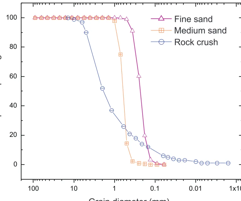
2.3 Sediment characterisation
188We used two different sands to evaluate the effect of grain size and a poorly sorted material – 189
rock crush – to investigate the effects of a broad grain size distribution. Specifically, the 190
substrates used were: (i) Leighton Buzzard DA 16/30, a medium sand, (ii) Leighton Buzzard 191
RH T, a fine sand and, (iii) poorly sorted rock crush containing particles ranging in size from 192
fine silt to gravel. The sands are both composed of quartz grains and their size distributions 193
were measured by dry sieving (Atkinson, 2008). The rock crush is a mixture of crushed 194
igneous rocks, including basalt and granite. The grain size distribution of the rock crush was 195
measured using the wet sieve method and hydrometer to British Standard BS1377 Part 196
4:1990 by Soil Property Testing Ltd, Huntingdon, UK. Quantitative grain size data are shown 197
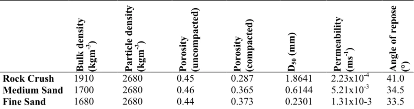
in Table 1 and Fig. 2. 198
<FIGURE 2 AND TABLE 1 HERE> 199
The permeability of each material was measured using the falling head method (Head, 200
1982) by Soil Property Testing Ltd, Huntingdon, UK and is shown in Table 1. We use the 201
permeability of the materials as a minimum estimate of their infiltration rate. Under 202
equilibrium conditions the infiltration rate approaches the permeability (Youngs, 1964), 203
however the instantaneous infiltration rate of each of the materials is a function of both the 204
permeability and the sorptivity of the material. For the two sands, it is reasonable to assume 205
that a constant factor should apply, however for the rock crush, this factor could be slightly 206
larger (Culligan et al., 2005). Bulk density, particle density and porosity (Table 1) were 207
ascertained prior to permeability testing using the standard methods as described in Head 208
(1982). The angle of repose of the materials was measured by gently forming a loose conical 209
pile of sediment and averaging two measurements of the incline of the slopes formed. The 210
angle of repose was very similar for the two sands (33-35°), but much greater for the rock 211
crush (41°). The angularity of the sediments was determined by microscopy: the sand grains 212
were sub-rounded to well-rounded in shape; the rock crush had sub-angular to angular grains. 213
Grain compositions and grain size distributions have been shown to be widely 214
variable on Mars from in-situ observations from Viking (Clark et al., 1977; Moore and 215
Jakosky, 1989) through to the Mars Exploration Rovers (e.g. Cabrol et al., 2007; Jerolmack et 216
al., 2006; Sullivan et al., 2008) and from remote sensing observations that use thermal inertia 217
as a proxy for grain size (e.g. Fergason et al., 2006). Grain sizes range from clay-size (Pike et 218
al., 2009) to boulders and can be very well sorted through to very poorly sorted. The 219
materials used as simulants are somewhat more restricted (e.g. Peters et al., 2008; Sizemore 220
and Mellon, 2008), but still have a range of physical and chemical properties. Although we 221
are exploring the effects of material parameters, rather than simulating martian regolith per 222
se, the physical properties of the materials used in this study are certainly within the bounds 223
of possible martian surface materials. Very fine material was avoided due to technical and 224
health and safety restrictions, rather than its inapplicability to Mars. 225
3 Results
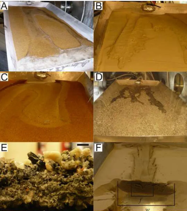
2263.1 Summary
227Table 2 provides a summary of the results for all the experiments performed in this study. For 228
each sediment type, three experiments were performed at low temperature and low pressure, 229
one was performed at room temperature but low pressure, and one performed at ambient 230
pressure and room temperature. Within the low temperature/low pressure experiments, two 231
were performed with water at ~ 5 ºC and one with water at ~ 0.5 ºC. An example of the 232
appearance of the sediments at the end of each experiment is shown in Fig. 3, with labels to 233
explain the terms used in the text. 234
Our experiments had a range of Reynolds Numbers (Table 2): only the medium and 235
fine sands were fully turbulent (Re > 1000) for their maximum values of Re. The flows in the 236
sands were usually partially turbulent and the flows over the rock crush were always laminar 237
(Re < 100). The Froude Numbers of our flows (Table 2) ranged from 0.06 – 1.19, but only 238
flows in the rock crush experienced critical (Fr > 1) conditions. The rest of the flows were 239
subcritical (Fr < 1) and the fine sand had the lowest range of Froude Number (0.14 - 0.69). 240
<FIGURE 3 and TABLE 2 HERE> 241
3.2 Observations: low temperature and low pressure experiments
2423.2.1 All Sediment Types 243
For all sediment types the water was seen to exude gas bubbles (e.g. video 1) and to form ice 244
on introduction into the chamber, indicating simultaneous boiling and freezing. Observations 245
of the sediment body after the experiments were completed confirm that water was able to 246
infiltrate only a small depth into the bed before it froze, forming an icy-sediment lens over 247
which the rest of the flow progressed (Fig. 3). The sediments underneath were still dry. 248
Boiling resulted in the formation of bubbles within the ice and the frozen sediments. Where 249
water collected at the end of the tray (e.g. video 2), the resulting ice was extremely bubble-250
rich and opaque on top with an underlying translucent, bubble-free layer. This structure is 251
similar to those described by Cheng and Lin (2007) and Bargery (2008) in experiments 252
performed with standing bodies of water at low temperature and low pressure. 253
<VIDEO 1 and VIDEO 2 HERE> 254
3.2.2 Fine and Medium Sand 255
For the sand substrates the flow initially spread out laterally across the surface at the top of 256
the tray and then progressed down the slope along one or more principal paths (video 1 and 257
video 3). Bubbling water was seen to flow over the surface and, towards the end of the 258
experiment, formed distinct channels (Figs. 3 and 4A). In the case of the fine sand the flow 259
was pulsing and migrated laterally forming lateral levees. In the medium sand, by 260
comparison, two broad channels were formed relatively quickly. The flow was more 261
continuous and did not migrate laterally (compare video 1 fine sand and video 3 medium 262
sand), depositing low lateral levees. In both cases, the channels and levees were linear rather 263
than sinuous. When the flow encountered the backstop, water and sediment spread laterally 264
and backed up, collecting into a pool extending 10-20 cm upstream from the bottom of the 265
tray (Fig. 4A). This ponded water bubbled vigorously in most cases, forming large bubbles 266
(~ 1 cm for medium sand and 1-5 cm for medium sand), until the surface froze (video 2). 267
<FIGURE 4 and VIDEO 3 HERE> 268
The fine sand formed more small lateral lobes than the medium sand (Figs. 4B and 269
4C). For the ~ 0.5 ºC water runs the deposits were rougher and formed a fan of icy slush. In 270
these experiments almost no water ponded at the end. Runs that used the warmer 5 ºC water 271
often showed ponding of water at the end of the test bed that resulted in a wedge of ice. The 272
icy wedges at the end of the flow had dry sediment underneath, showing that the flow had not 273
penetrated to the base of the tray. 274
3.2.3 Rock Crush 275
The flow initially spread out laterally as for the sands. However, the flow then progressed as 276
multiple digitate lobes (Fig. 4D), which then quickly coalesced into a sheet flow, rather than 277
channelized flow (in contrast to flow over the sand beds) as shown in video 4 and Fig. 5. On 278
one occasion, small but detectable channels and fans did form, but these were within the 279
sheet-like flow. It is notable that the depositional fan in this case was entirely composed of 280
the finer material; coarser material was not transported. As the flow encountered the backstop 281
the water backed up to 20-25 cm upstream and ponded. This water bubbled gently with small 282
bubbles forming (1-5 mm) until an ice sheet formed over the top (video 5). 283
<FIGURE 5, VIDEO 4 and VIDEO 5 HERE> 284
Close observation revealed that the flow front progressed by travelling around the 285
larger clasts, before inundating them as the flow matured. In cross section, the icy sediment 286
lens contained a concentration of coarser clasts at the top (Fig. 4E), indicating the surface had 287
been washed free of fines. Bubbles were not observed breaking the surface in the rock crush, 288
but were observed in the ice lens and ice wedge deposits at the end of the tray. Water was 289
observed to pond at the end of the tray irrespective of the initial water temperature. The ice 290
wedge which then formed at the end of the tray penetrated through the sediment to the base 291
of the tray, except when the water was cooled to ~ 0.5 ºC, when 1 - 2 cm of dry sediment was 292
left underneath. 293
3.3 Observations: control experiments performed at 1) Earth ambient
294conditions and 2) low pressure and Earth ambient temperature
2953.3.1 All Sediment Types 296
The water was able to infiltrate into the sediments for all the experiments. There were 297
therefore some obvious differences from the experiments performed at low temperature and 298
pressure: 299
(i) flows were slower to progress down slope for a given sediment type (Table 2).
300
(ii) there was no ponding of water at the end of the tray.
301
(iii) wet haloes of sediment formed around the flows, extending downwards as
302
well as sideways (Fig. 4F). 303
(iv) the flows did not cover such a large spatial area, Fig. 6.
304
Together these suggest that wetting, infiltration and subsurface flow were more 305
important than the subfreezing experiments. 306
<FIGURE 6 HERE> 307
3.3.2 Fine and Medium Sand 308
Compared to the low temperature/low pressure experiments the flows in sands remained 309
confined laterally, both initially and throughout the flow duration, Fig. 5. For the fine sand 310
the flows had some lateral migration, but much less than the low temperature/low pressure 311
runs (video 1). The lateral migration of flows across the medium sand was even more limited 312
(video 3). Both flows built lateral levees and were somewhat pulsing in nature. In cases 313
where the flow encountered the backstop a fan of sediment built up, propagating laterally (~ 314
15 cm) and upstream. None of the flows on the medium sand substrate reached the end of the 315
tray under ambient temperature and pressure conditions. In all cases water infiltrated 316
downwards to the base of the tray beneath all the flows. During the ambient temperature/low 317
pressure experiment both sands contained bubbles and had surface blisters. The bubbles and 318
blisters were present in the percolation halo as well as along the flow path. 319
3.3.3 Rock Crush 320
The flow for the rock crush was very similar in style to the experiments at low 321
temperature/low pressure (video 4). Initially the flow spread both downstream and laterally, 322
and continued to do so as the flow progressed. The flow propagated in all directions forming 323
a radial flow front, elongate in the downstream direction. In contrast to the low 324
temperature/low pressure experiments, the flow was not initially digitate. The wet sediment 325
surface was observed to bubble during the ambient temperature/low pressure experiments 326
(video 6). For the ambient temperature and pressure experiment the flow did not reach the 327
end of the test bed (video 4) and it barely reached the backstop in the low pressure 328
experiment. Not enough flow reached the backstop for it to have significant influence on the 329
progress of the flow (video 6). 330
<VIDEO 6 HERE> 331
The flows on the rock crush substrate progressed much more slowly for both the ambient 332
temperature experiments than they did for the cold runs (Table 2). The flow was more 333
channelized in the uppermost portion than for the low temperature/low pressure experiments. 334
Infiltration in both cases resulted in the water penetrating to the base of the tray under the 335
flow lobe. Despite the boiling observed in motion during the ambient temperature/low 336
pressure experiments, no bubbles were preserved within the rock crush because there was no 337
ice to preserve them. 338
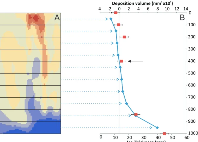
4 Data analysis
3394.1 Volume calculation
340The x, y and z coordinates from the measured cross profiles were interpolated into a gridded 341
surface using the Kriging method in Surfer 8 software. This method has provision to allow 342
for anisotropy in data collection (a greater density of sampling was used post-experiment in 343
some cases). A 1 cm grid size was chosen as appropriate for the wavelength of changes 344
observed and applied to all the surfaces. To calculate the volume of erosion and deposition 345
for each experiment the pre-experiment surface was subtracted from the post-experiment 346
surface. The results for the overall volumes are given in Table 2 and an example of the spatial 347
results is mapped in Fig. 7. 348
<FIGURE 7 HERE > 349
The deposition volumes are much larger than the erosion volumes for low 350
temperature/low pressure experiments. Most of the additional volume can be accounted for 351
by the ponded water at the base of the flow, and by large cavities that formed in the ice 352
wedge as a result of boiling. Within the bounds of error (± 1 mm in height measurements) the 353
erosion and deposition balance out for the ambient temperature/ambient pressure experiments 354
(Fig. 8C). The data show consistent excess in deposition volume for all the ambient 355
temperature/low pressure experiments: this may represent an increase in volume through 356
incorporated gas, although we note that these values are comparable to the estimated 357
measurement error. 358
Because the deposition data include additional ice, water and gas, we used the erosion 359
volume to estimate the volume of sediment transported. This erosion volume was derived for 360
each experiment simply by summing all the pixels in each difference map that had negative 361
displacements. From this we generated an erosion rate, based on the estimated volume of 362
material removed normalised to the tray area and the duration of the flow. Using the 363
estimated removed sediment volume, the material porosity and the volume of water we made 364
an estimate of the sediment concentration in the flows. 365
From the spatial distribution of erosion and deposition we also determined the 366
“erosion distance” - the horizontal distance that each flow travelled before changing from net 367
erosion to net deposition (Fig. 7). The erosion distance is another measure of the erosional 368
ability of the flow. This was performed by dividing the tray area into segments (Fig. 7) and 369
summing all the erosion and depositional pixels within each segment. This determined 370
whether each segment was dominated by erosion or by deposition, as well as the net erosion, 371
or deposition. The horizontal distance at which the transition occurred was determined 372
graphically. In reality this is a minimum estimate, because some of the surface lowering by 373
erosion is countered by ice expansion and bubble formation, which masks some of the areas 374
which actually had small net erosion. 375
4.2 Erosion
376For all the experiments this erosion rate was between 0.002 and 0.055 mm.s-1 and the erosion
377
distance was between 50 and 650 mm from the source of the flow. In general, the rock crush 378
shows much lower erosion (rate, or distance) than either of the sands (Fig. 9 and Table 2). 379
This result is consistent with the results of Shields (1936) and Kirchner et al. (1990) that 380
larger particles and more angular particles require more stress to move. For the low 381
temperature/low pressure experiments, all sediment types had higher erosion rate and 382
distance when using the warmer water (Fig. 9). However, the patterns of erosion rates for the 383
different experiments varied between each sediment type: (1) in the sub-freezing experiments 384
the erosion rate and distance in the medium sand was on average greater than in the ambient 385
experiments, (2) the fine sand shows a similar trend, but less marked and, (3) for rock crush 386
the erosion rate was lowest for the low temperature/low pressure with colder water, and all 387
the other experiments have higher and very similar erosion rates. 388
<FIGURES 8 and 9 HERE> 389
For the subfreezing experiments the erosional parts of the flow had a thinner ice lens 390
than the depositional parts of the flow (Figs. 7 and 8). The ice lens was thickest where 391
deposition was greatest – usually at the end of the tray (Figs. 7 and 8). The icy-sediment lens 392
formed at the base of the flow ranged from 0.5 - 3.5 cm thick for both the sand types and was 393
thinner (0.5 - 1.0 cm) and more uniform for the rock crush. 394
4.3 Runout distances
395The runout distances were calculated by projecting the flow speed (as calculated by the time 396
for the flow front to reach the base of the tray) over the duration of the experiment. In all 397
cases the runout distance is greater for each material type under sub-freezing conditions than 398
under ambient temperature conditions (Fig. 10). This agrees with the qualitative observations 399
of ponding occurring at the end of the subfreezing experiments, but not occurring at ambient 400
temperatures (documented in Sections 3.2 and 3.3). This effect is most marked in the medium 401
sand. In addition when comparing the ambient temperature experiments performed at 402
different pressures, the runout distances for the sands seem to be greater at low pressure than 403
at ambient pressure (Fig. 10). However, this result should be treated with some caution as 404
only a limited number of experiments were performed. 405
<FIGURE 10 HERE> 406
5 Discussion
4075.1 Transport dynamics under low temperature and low pressure
408The formation of an ice lens at the base of the flow retarded infiltration, leading to more 409
surface flow and therefore faster down slope flow propagation. We infer the lack of 410
infiltration from the presence of dry sediments beneath the ice lens and from the pooling of 411
excess water at the end of the tray. Infiltration experiments performed on soils under ambient 412
terrestrial pressure conditions by McCauley et al. (2002) showed a similar distinct decrease in 413
infiltration rate for freezing soils. If our test bed had been longer, the flows under freezing 414
conditions would have had a significantly greater runout distance than those under ambient 415
temperatures, as indicated by our calculations in Section 4.3. Freezing temperatures therefore 416
have a fundamental affect on the behaviour of the flow, if not on the actual erosion rate. 417
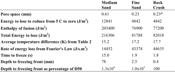
We can estimate the depth to the freezing front by using Fourier’s law of heat 418
conduction. Assuming that the water is in contact with a semi-infinite plain of cold 419
homogenous material (whereas in reality it has infiltrated into the pores of a granular 420
mixture), under steady-state conditions, we can simplify Fourier’s law to a heat loss per unit 421
area (q) which gives: 422
q =ΔE/Δt = k A (T1-T2) / x (1)
423
where T1 (5°C) is the temperature of the water, T2 (-20°C) the temperature of the substrate, k
424
the thermal conductivity of the water (0.58 W/mK), A the area of contact, x the thickness of 425
the material, ΔE the energy change and Δt the time duration. If we assume that a thickness of 426
one pore space must freeze to halt infiltration, we can use the pore space as the thickness, x. 427
This is the distance over which the temperature must to be reduced to zero and hence we can 428
calculate how much energy must be lost (ΔE). We need to account for the energy loss due to 429
both the temperature drop and the enthalpy of fusion, for which we use a specific heat 430
capacity, C = 4.210 kJ/kg.K, a standard enthalpy of fusion, H = 333.55 kJ/kg and a density, ρ 431
= 1000 kg/m3 for water at just above 0 °C. Hence:
432
ΔE = ρx (H + C T1) (2)
433
and combining Eqs. (1) and (2) and rearranging gives: 434
Δt = ρx2 (H + C T1) / k A (T1-T2) (3)
435
By using Eq. (3), we can estimate for each sediment type how much time is required to freeze 436
such a layer and to what depth the water should have infiltrated when this occurs (using the 437
permeability values listed in Table 1). The calculation is laid out for each material in Table 3. 438
Despite the large number of simplifying assumptions, the depths to the bottom of the ice layer 439
are broadly supported by our observed ice thicknesses (Fig. 11), both in terms of ranking and 440
order of magnitude. However, our calculations over-estimate the depth of penetration into the 441
medium sand and underestimate for the fine sand and rock crush. This could be due to an 442
under-estimate of the instantaneous infiltration rates for the fine sand and rock crush 443
(sorptivity is higher for smaller pores), an over-estimate of the pore size for the medium sand, 444
or the violation of the other assumptions inherent in the calculation (planar continuous 445
material and steady state conditions). 446
<TABLE 3 & FIGURE 11 HERE> 447
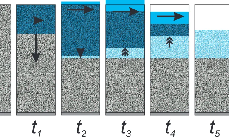
Starting from this mechanism we can build a simple process model. A schematic 448
diagram representing the important stages in the evolution of the flow is shown in Fig. 12. 449
The ice barrier forces the flow to be in the regime of saturation overland flow (Dunne and 450
Leopold, 1978), because the depth to saturation is restricted by the ice lens. Under ambient 451
conditions this regime is only experienced by the medium sand. In this case the depth to the 452
base of the tray is so great that only limited amounts of overland flow occurs. If the medium 453
sand was infinitely deep, the flow would not have propagated very far at all (~ 10 cm). 454
Hence, the greatest difference is seen for the runout and erosion for the medium sand. For the 455
fine sand and rock crush the discharge is sufficient to counteract the losses by infiltration, and 456
overland flow continues ("Horton overland flow": Horton, 1945). Hence the transition to 457
saturation overland flow under sub-freezing conditions increases the runout, but does not 458
always affect the erosion. The reason for the variations in erosion-rate dependence is 459
explored below. 460
<FIGURE 12 HERE> 461
It would be expected that the formation of a basal icy-lens at such shallow depths 462
would retard erosion as it turns a cohesionless substrate into one with cohesion. However, the 463
propagation of the freezing front is counterbalanced by the erosion rate of the unfrozen, yet 464
saturated material (Fig. 12-t4). It would be expected that once the saturated substrate above
465
the growing ice has been removed, that thermal erosion would come into play. Thinner ice 466
sheets were observed nearer the top of the tray (Figs. 7 and 8) and in the channels and this 467
could be explained using thermal erosion arguments. In addition, we observed that the 468
warmer, 5 °C water onto the cold substrate caused more erosion than the colder water at ~ 0.5 469
°C (Fig. 13). This can be explained using both arguments of faster propagation of the freezing 470
front and less efficient thermal erosion. The rates of thermal erosion calculated from 471
experimental and numerical modelling results of Costard et al. (1999) and Randriamazaoro et 472
al. (2007), range upwards from 0.4 mm/min (6.7x10⁻⁶ m/s). However, Randriamazaoro et al.
473
(2007) showed that thermal erosion increases with Re and the flow regimes in their study 474
have much greater Reynolds numbers (Re > 6345) compared to our flows’ Reynolds numbers 475
(5-1645; Table 2). Hence, their minimum rate provides an absolute maximum when applied 476
to our flows and, because it is much lower than our erosion rates (1.56x10⁻⁴ –
477
3.58x10⁻³ m/min), we infer that the thermal erosion mechanism is not usually dominant.
It is generally expected that erosion rates should be greater for greater flow rates, but 479
this was not always the case in our experiments. This could be due to the freezing bed 480
introducing two competing effects: it increases the flow rate, yet also impedes the erosion by 481
freezing the particles to the bed (hence the slower thermal erosion mechanism becomes 482
dominant). The dominance of one effect over the other is probably related to the freezing 483
rate. As shown in Fig. 13 the erosion decreases as the difference in temperature between 484
sediment and water decreases (the lower the difference the colder the water). Hence, the 485
armouring of the bed is most effective at reducing erosion when the temperature difference is 486
lower, with the water closer to freezing resulting in a faster propagation of the freezing front. 487
<FIGURE 13 HERE> 488
5.2 Flow runout distances
489Another way of looking at the dynamics of these flows is to consider the mass balance of the 490
flow. If we consider a discharge (q) per unit width, w, then this results in the following: 491
q = qin –Vix – Vevx - Vfrx (4)
492
where qin is the initial discharge, x is the distance from the outlet, Vi is the rate of loss due to
493
infiltration, Vev the rate of loss due to evaporation and Vfr the rate of loss due to freezing. This
494
assumes steady flow conditions with no lateral changes in width. These approximations are 495
not valid for our experiments, however a full unsteady model would require a 3D 496
morphodynamic model. This would include conservation of momentum, conservation of 497
sediment, and constitutive equations for these highly concentrated (20 % for fine sand and 30 498
% for medium sand), self channelized flows. Such an attempt is beyond the scope of this 499
analysis. Instead of a full solution, our goal is to provide a simple framework in which to 500
assess the relative contributions of discharge, freezing, evaporation and infiltration to the 501
flow runout distances. Despite these simplifying assumptions, the analysis yields insightful, 502
albeit qualitative, results, as detailed below. 503
Using the mass balance Eq. (4), we can consider the length over which the flow 504
discharge falls to zero, from this we can ascertain: 505
L = qin / (Vi + Vev + Vfr) (5)
506
where L is the total length of the flow. 507
From the experiments to investigate the evaporation of standing bodies of water under 508
martian atmospheric pressure and at 0°C by Sears and Moore (2005) the value of Vev should
509
be ~ 2.0x10⁻⁷ m/s. In our experiments, Vfr changed as a function of downstream distance as
510
shown by the increasing ice lens thickness in Figs. 4, 7 and 8. To estimate the range in Vfr, we
511
use both the minimum and maximum value of thickness of sediment that froze at the base of 512
the channels over 30 s for the sands and the rock crush. Hence, considering also the material 513
porosity (but not the included bubbles), gives mean freezing rates ranging from 6.6x10⁻⁴ to
514
1.6x10⁻⁴ m/s for fine sand, from 6.1x10⁻⁴ to 2.3x10⁻⁴ m/s for medium sand and from 2.7x10⁻⁴
515
to 6.0x10⁻⁵ m/s for rock crush. From Table 1 infiltration rates range from 5.21x10⁻³ to
516
2.23x10⁻⁴ m/s. Therefore, it can be seen that evaporation is relatively unimportant when
517
compared to the other losses, by at least three orders of magnitude. When no freezing occurs 518
during the flow Vfr is zero and Vi is at its maximum. Conversely under sub-freezing
519
conditions Vi approaches zero and the loss term is dominated by Vfr.
520
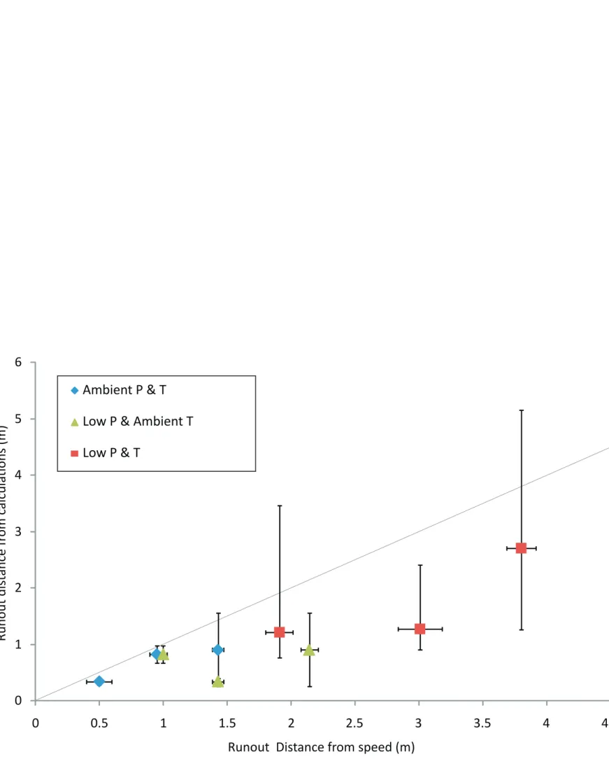
Using the above values for the freezing rates, evaporation rates and infiltration rates, we 521
have used Eq. (5) to predict the expected runout distance for each of our experiments. In the 522
subfreezing experiments we set Vi equal to zero and in the experiments performed at room
523
temperature, Vfr was set to zero. Figure 14 is a plot of this predicted runout distance against
524
the runout distance as calculated from the flow speed. There is good agreement between the 525
two runout distances for the ambient temperature and pressure experiments. The runout 526
distance is greater for the ambient temperature/low pressure experiments than predicted by 527
Eq. (5), a possible explanation for this is presented in Section 5.3. The predicted runout 528
distance for the sub-freezing experiments is also generally an underestimate. The predicted 529
runout using a minimum freezing rate (as indicated by the maximum vertical extent of the 530
error bars in Fig. 14) produces a much better match to the calculated runout distances for the 531
rock crush, but an overestimate for the two sands. 532
<FIGURE 14 HERE> 533
5.3 Influence of low pressure
534Our experimental data suggest that pressure is not as important as temperature for controlling 535
the gross behaviour of the flows. However, the flow propagation speed was greater at low 536
pressure than at ambient pressure. For example, the flows in the experiments performed with 537
medium sand propagated to the end of the tray at ambient temperature/low pressure, but only 538
propagated to ~ 50 cm under ambient temperature/ambient pressure (Table 2). The effect is 539
less marked (but still apparent) for the rock crush and the fine sand. A possible explanation 540
for enhanced flow at low pressure is that the formation of bubbles within the sediment 541
inhibits infiltration as the water boils. This effect was noted by Prunty and Bell (2007) who 542
found unexpectedly low infiltration rates in their low-pressure infiltration experiments. It is 543
well established that formation of bubbles from exsolved gases can greatly reduce aquifer 544
permeability, for example Ronen et al. (1989) found a reduction of infiltration rates in sands 545
from 45 m/day to 2 m/day resulting from biotic bubble formation and Amos and Ulrich 546
Mayer (2006) found a reduction of up to 25% from abiotic bubble formation. 547
As detachment bubble size for boiling water increases with decreasing atmospheric 548
pressure, it is possible that the bubble size of water on the martian surface is equivalent to or 549
greater than the sediment pore size of the substrate, and hence boiling is able to inhibit 550
infiltration. Prodanovic et al. (2002) ran experiments involving supercooled water (-30°C) at 551
pressures of <3 mbar and found bubble detachment diameters of 0.3-0.5 mm. Hence it is 552
certainly possible that bubble detachment size is greater than the pore size in our 553
experiments. Another possible explanation might be that small bubbles in the flow caused the 554
flow to be less dense, again reducing infiltration – although we note that this also should 555
cause flow propagation to be slower and is contrary to the observations. 556
5.4 Implications at field scale
557Two features on Mars, gullies and slope streaks, could be forming at present and hence the 558
results from our experiments could throw some light on their formation processes. Gullies on 559
Mars are kilometre-scale features that resemble gullies that form on Earth due to overland 560
flow of liquid water, or highly concentrated flows of sediment and water (debris flow). They 561
have been widely studied as such since their discovery by Malin and Edgett (2000). Initially 562
they were proposed to have formed by the outflow of water from a subsurface aquifer 563
(Heldmann and Mellon, 2004; Malin and Edgett, 2000). However, recent observations on 564
morphology, distribution and their setting within landform assemblages (e.g. Balme et al., 565
2006; Dickson and Head, 2009) has strongly suggested that they originate from melting of ice 566
under recent climate excursions. Other explanations for their origin include dry (or carbon 567
dioxide assisted) granular flow (e.g. Pelletier et al., 2008), but these mechanisms do not 568
produce all of the key morphologies and do not explain their distribution. Key to both the 569
aquifer model and the melting models is the efficiency of water in transporting sediment 570
under martian surface temperature and pressure. 571
Slope streaks are flow-like features that contrast with the underlying material (mostly 572
having lower albedo, although some have higher albedo) that propagate downhill, being 573
diverted around obstacles and affected by topography (e.g. Sullivan et al., 2001). They form 574
with great frequency on Mars and have been observed to both form and to be erased 575
(Aharonson et al., 2003) on Mars in time periods of less than 10 years. Slope streaks were 576
first seen in Viking Orbiter images (e.g. Morris, 1982) and were found to be associated with 577
dusty areas on the planet (e.g. Ferguson and Lucchitta, 1984). These features have primarily 578
been interpreted as being formed by a dry mass wasting process (e.g. Chuang et al., 2007), 579
however some recent work has indicated that liquid water might be involved in their 580
formation (Kreslavsky and Head, 2009). 581
Although our experiments are not replicates of the martian surface, it is useful to use 582
Eq. (5), with the rates calculated from our experiments, to estimate the discharge that might 583
be required to generate flows of this type over longer distances. Although mass balance (i.e., 584
Eq. 5) should hold on Mars, there are caveats to directly applying the rates from our 585
experiments to Mars, which are discussed in detail in Section 5.5. For sub-freezing 586
conditions, similar to our experiments, when Vi ~ 0, gullies or slope streaks of 1 km in length
587
and 20 m in width would require a discharge of between 670 ls-1 and 13 000 ls-1, depending
588
on the sediment type and freezing rate, for flow to occur from top to bottom. However, under 589
non-freezing conditions, when Vfr = 0, discharges in this system would need to be increased
590
to between 4500 ls-1 and 100 000 ls-1 depending on the sediment type. Some slope streaks
591
have smaller dimensions and thus smaller discharge requirements, for example slope streaks 592
of 5 m wide and 50 m long would require 8 to 116 ls-1 with a freezing substrate and 56 to
593
1300 ls-1 without. The large ranges in discharges from our calculations emphasise the strong
594
influence that infiltration rates have on the fluid loss parameter and on overall runout 595
distances, both in terms of material type and in terms of the presence of an impermeable layer 596
(in our calculations an ice layer formed by the flow). Impermeable layers could also be 597
formed by permafrost or shallow bedrock and hence would not necessarily have a large 598
freezing loss associated with them. However, these impermeable layers would be expected to 599
be found at greater depths, hence the reduction in infiltration would be less marked and occur 600
with a time delay. 601
Some flow rate estimates have been made for gullies on Mars, for example, Heldmann 602
et al. (2005) estimate 30 000 ls-1 for a generic gully, Hart et al. (2009) estimate 750 – 83 000
603
ls-1 for bankfull discharge from gully measurements at Lyot crater and Parsons and Nimmo
604
(2010) give an estimate of 45 000 ls-1 from modelling sediment transport to generate a
605
generic gully. Our mass-balance calculations based on our experimental results broadly 606
support these flow rates. However, our calculations suggest that such large discharges are not 607
required if the system is freezing. Heldmann et al. (2005) invoke these large flow rates to 608
compensate for freezing and evaporative losses and to explain the formation of deep, wide 609
channels in single events. Hart et al. (2009) generated large discharges to fulfil their 610
assumption of bankfull discharge, without consideration of loss parameters. Parsons and 611
Nimmo (2010) do not use a fluid loss parameter, as they consider losses as insignificant over 612
the duration of gully formation. Our experiments emphasise the importance of considering 613
infiltration rates, omitted from both these studies, when performing this kind of calculation. 614
It has been previously recognised that fluid loss is an important parameter in terms of 615
modelling gullies on Mars and has a great influence on the runout distance and morphology 616
of the resulting flow (Kolb et al., 2010; Pelletier et al., 2008). Our work shows that under 617
sub-freezing conditions there is some fluid loss through freezing, but also shows that fluid 618
loss is reduced through the inhibition of infiltration. Our experiments highlight that 619
evaporative losses are not important compared to losses due to freezing and infiltration and 620
that careful consideration of these terms will be necessary in future modelling. The minimum 621
fluid loss values used by Kolb et al. (2010) and Pelletier et al. (2008) are at the maximum of 622
our estimated fluid loss and only our highest infiltration rate (medium sand) approaches the 623
fluid loss parameter used by Heldmann et al. (2005), and even then solely under non-freezing 624
conditions. We maintain that further work is required to accurately define the quantitative 625
limits of the fluid loss term under martian temperature and pressure for use in modelling 626
studies. 627
5.5 Caveats to up-scaling the experimental results.
628Our experiments were designed to investigate the effect of Mars-like pressure and 629
temperature on overland flow and sediment transport. Although we feel the results are robust, 630
care must be taken in extrapolating the results herein to natural systems that lie outside the 631
parameter space investigated. This is in part because designing and conducting experiments 632
within a low temperature and low temperature facility are necessarily at a scale smaller than 633
most natural systems of interest and so explore a limited range of parameter space. Below we 634
elaborate on these limitations and discuss future opportunities in experimentation. 635
Open-channel flows are typically scaled dynamically using the Reynolds number and 636
the Froude number (e.g., Chow, 1959). Each of our experiments had different ranges of 637
Reynolds numbers (Re) and within each experiment Re spanned a range of values (Table 2). 638
Only one experiment in the medium and one in the fine sand were fully turbulent (Re > 1000) 639
where Re was at its maximum. The flows in the sands were usually partially turbulent and the 640
flows over the rock crush were always laminar (Re < 100). Larger flows with fully turbulent 641
Re might be expected to have different runout lengths, not only because of their greater size, 642
but also due to changes in bed friction (Chow, 1959) and the rate of turbulent energy 643
dissipation to heat (Tennekes and Lumley, 1972). This notwithstanding, we saw no major 644
trend in our results with Re, indicating that perhaps these are second order effects as 645
compared to the changes in infiltration rate caused by freezing. Moreover, it has been argued 646
that many similarities exist in sediment bed morphodynmaics between laminar flows and 647
turbulent flows (Lajeunesse et al., 2010). 648
The Froude Numbers of our flows ranged from 0.06 – 1.19, a large range of parameter 649
space from subcritical to critical conditions. Subcritical Froude number are much more 650
common in sediment-transport systems on Earth (Grant, 1997), but supercritical flows can 651
occur, especially on steep slopes. For martian gullies, models have explored a range of 652
Froude numbers including supercritical conditions (Heldmann et al., 2005; Kolb et al., 2010; 653
Parsons and Nimmo, 2010; Pelletier et al., 2008). Since the transition to supercritical flow 654
can significantly change flow hydraulics (e.g., by allowing hydraulic jumps) future work is 655
needed to explore this area of parameter space in more detail. 656
The above discussion of Re and Fr implicitly assumes dilute (c<<1) Newtonian-flow 657
conditions. It is possible that some of the gullies on Mars are carved by highly concentrated 658
non-Newtonian flows (i.e., debris flows, e.g., Lanza et al., 2010) or dry avalanches (Treiman, 659
2003). In some of our experiments the sediment concentrations were high (Table 2), and 660
showed some non-Newtonian behaviour including granular snouts of flows and levees on the 661
sides of channels. It is less clear how to up-scale runout lengths and erosion of such flows, 662
given the complex interplay between particle-particle interactions and pore pressure (Hsu et 663
al., 2008; Iverson, 1997). These experiments were not designed to simulate gully formation 664
by dry avalanching. 665
The effect of changes in gravity on overland flow and sediment transport has been 666
explored by others (Burr et al., 2006; Komar, 1980). In general, it has been found that flows 667
will move slower under lower gravity, but that sediment weighs less, so that sediment 668
transport rates on Earth and Mars scale similarly. It is also expected that infiltration rates will 669
be slower under reduced gravity (Chan et al., 2004). However, we suspect that all of these 670
effects that result from different gravity for Mars conditions (by roughly a factor of three 671
from Earth conditions) should be small (by several orders of magnitude) in comparison to the 672
effect of reduced infiltration due to freezing, and therefore should not change substantially 673
the experimental findings. 674
In these experiments we have only tested three sediment types. However, the material 675
property that exerts the greatest influence on the experiments is the permeability of the 676
material. A secondary effect was the ability of the flow to entrain certain sizes of particles. 677
Where the flow was not able to entrain particles in our experiments (rock crush), flow 678
spreading occurred. This counter-acted the effect of reduced infiltration rate which would 679
otherwise have acted to further increase the runout distance. If we were to use a sediment that 680
was highly impermeable, with small to average grain size, a situation could occur in which 681
runout is maximised. However, we predict in this case that erosion would be slow, because 682
the bed would freeze quickly and erosion would progress mainly by slower thermal erosion 683
as the bed is melted again. 684
We also only tested one inclination angle of the test bed. Higher inclination should 685
increase the flow speed and slightly reduce the infiltration effects (Dingman, 1994). The 686
temperature of the test bed and fluids should also influence the results. Given a lower 687
sediment temperature the freezing front should occur at a shallower depth. We did vary the 688
input water temperature (5°C or 0.5°C), which also decreases the temperature difference. 689
However, the effects of the more rapid formation of an ice lens were possibly masked by the 690
effects of ice particles forming within the flow. 691
Using different fluids could have a significant effect on fluid behaviour. Various 692
compounds have been proposed to form solutions on Mars, which could facilitate the stability 693
of water at low temperatures. Suggested compounds include: perchlorates (Catling et al., 694
2009; Hecht et al., 2009), Calcium Chloride (Knauth and Burt, 2002), Sodium Chloride 695
(Sears et al., 2002), and Ferric Sulphate (Chevrier and Altheide, 2008) brines; organics (Jean 696
et al., 2008) and acids (Benison et al., 2008). These all have a higher viscosity than pure 697
water. For example Chevrier et al. (2009) found the viscosity of ferric sulphate solutions to 698
be between 7.0x10⁻³ and 4.6 Pa s at temperatures of 285-260 K. An increase in viscosity
would act to slow the flow rate for flows with Re < 103 and decrease infiltration (e.g., Jarsjö 700
et al., 1997; Lin et al., 2003). Flow rates for fully turbulent flows (Re > 103) are independent
701
of fluid viscosity(Tennekes and Lumley, 1972). The stability of these solutions at low 702
temperatures would prevent the formation of a basal ice lens and might even promote thermal 703
erosion of any permafrost at the base of the flow (Andersland et al., 1996). These factors 704
combined suggest that very careful investigation of the inherent infiltration rate of the 705
sediment type is needed in these cases. If infiltration is very large and there is no formation of 706
a basal ice lens, then discharges would have to be very high for fluids to be able to flow 707
overland and form features such as gullies. This could make the above fluids implausible 708
when considering gullies on isolated topography. 709
710
6 Conclusions
711These experiments highlight some potential pitfalls when considering water flows on the 712
surface of Mars. Specifically, when using a fluid loss parameter in modelling, careful 713
consideration should be given to the factors influencing infiltration in the flow bed, i.e. (1) its 714
temperature (2) the infiltration rate of the unconsolidated material, (3) the presence or 715
absence of an impermeable layer and (4) the depth of such a layer if present. 716
We have found that water flowing over a freezing substrate behaves very differently 717
from water flowing over a warm bed. In the former case, water freezes at a shallow depth in 718
the substrate, impeding infiltration, causing the flow to propagate faster and further that it 719
would under ambient terrestrial conditions. This suggests that fluvial flow features on Mars 720
could be formed by volumes of liquid an order of magnitude less than for similar-length 721
flows on the Earth. 722
In addition to the effects of sub-freezing conditions we have found that low pressure 723
conditions also act to change the flow dynamics, but less dramatically than low temperature. 724
We found that flows are faster with a greater runout at low pressure/ambient temperature. We 725
hypothesise that infiltration is impeded by the formation of bubbles at the base of the flow, 726
but further work needs to be done to confirm this mechanism. Again, this suggests that 727
smaller volumes of water are required to create long flows on Mars than on the Earth. 728
Our experiments indicate that previous estimates of gully discharges are within the 729
upper estimates of those indicated by our analysis, but that the assumptions inherent in these 730
earlier calculations have underestimated the factors influencing the fluid loss parameter, 731
especially the infiltration rate. Further experimental work needs to be done to further 732
constrain the factors influencing fluid loss on the surface of Mars. 733
734
7
Acknowledgements
735We thank two anonymous reviewers for their comments which greatly improved this 736
manuscript. This work would not have been possible without a postgraduate studentship grant 737
from the U.K. Natural Environment Research Council (NERC). We gratefully acknowledge 738
the support of the staff at the Open University’s Research Design and Engineering Facility 739
and technical staff at Planetary and Space Science Research Institute. We thank Luther 740
Beegle for sharing his raw data on grainsize analysis of JSC-1 and MMS Mars simulants and 741
Karl Atkinson for allowing us to use his grainsize analyses results. We thank the staff at Soil 742
Property Testing Ltd., Huntingdon, UK for performing the permeability testing and grainsize 743
analysis. We are grateful to Helen Townsend for her assistance in the laboratory. 744