Assessment of impacts of climate change on water resources ? a case study of the Great Lakes of North America

(1)

HAL Id: hal-00298780

https://hal.archives-ouvertes.fr/hal-00298780

Submitted on 11 Oct 2006

HAL is a multi-disciplinary open access

archive for the deposit and dissemination of sci-entific research documents, whether they are pub-lished or not. The documents may come from teaching and research institutions in France or abroad, or from public or private research centers.

L’archive ouverte pluridisciplinaire HAL, est destinée au dépôt et à la diffusion de documents scientifiques de niveau recherche, publiés ou non, émanant des établissements d’enseignement et de recherche français ou étrangers, des laboratoires publics ou privés.

Assessment of impacts of climate change on water

resources ? a case study of the Great Lakes of North

America

E. Mcbean, H. Motiee

To cite this version:

E. Mcbean, H. Motiee. Assessment of impacts of climate change on water resources ? a case study of the Great Lakes of North America. Hydrology and Earth System Sciences Discussions, European Geosciences Union, 2006, 3 (5), pp.3183-3209. �hal-00298780�

(2)

HESSD

3, 3183–3209, 2006 Assessment of impacts of climate change on water resources

E. McBean and H. Motiee

Title Page Abstract Introduction Conclusions References Tables Figures J I J I Back Close

Full Screen / Esc

Printer-friendly Version Interactive Discussion

Hydrol. Earth Syst. Sci. Discuss., 3, 3183–3209, 2006 www.hydrol-earth-syst-sci-discuss.net/3/3183/2006/ © Author(s) 2006. This work is licensed

under a Creative Commons License.

Hydrology and Earth System Sciences Discussions

Papers published in Hydrology and Earth System Sciences Discussions are under open-access review for the journal Hydrology and Earth System Sciences

Assessment of impacts of climate change

on water resources – a case study of the

Great Lakes of North America

E. McBean1and H. Motiee2,*

1

University of Guelph-Guelph, Ontario, N1G 2W1, Canada 2

Power and Water University of Technology (PWUT), Tehran, Iran *

now at: University of Guelph, Ontario, N1G 2W1, Canada

Received: 28 August 2006 – Accepted: 1 September 2006 – Published: 11 October 2006 Correspondence to: E. A. McBean (emcbean@uoguelph.ca)

(3)

HESSD

Full Screen / Esc

Abstract

Historical trends in precipitation, temperature, and streamflows in the Great Lakes are examined using regression analysis and Mann-Kendall statistics, with the result that many of these variables demonstrate statistically significant increases ongoing for a six decade period. Future precipitation rates as predicted using fitted regression lines

5

are compared with scenarios from Global Climate Change Models (GCMs) and demon-strate similar forecast predictions for Lake Superior. Trend projections from historical data are, however, higher than GCM predictions for Michigan/Huron. Significant vari-ability in predictions, as developed from alternative GCMs, is noted. Given the general agreement as derived from very different procedures, predictions extrapolated from

his-10

torical trends and from GCMs, there is evidence that hydrologic changes in the Great Lakes Basin are likely the result of climate change.

1 Introduction

The Great Lakes of North America, namely Lake Superior, Huron, Michigan, Erie and Ontario, represent one of the most important water resources in the world, and provide

15

water for multipurposes for more than fifty million people in eastern North America. Combined, the Great Lakes and their connecting channels comprise the largest fresh surface water system on earth (Fig. 1), holding approximately 20 percent of the world’s fresh surface water supply (De Lo ¨e, 2000; GLIN, 2005). As an indication of the enor-mous size of the lakes, the estimated cumulative volume of the five lakes is 6×1015

20

(six quadrillion) gallons which is sufficient water to flood North America to a depth of 1 metre. The diversity of uses and the magnitude of the Great Lakes system interactions are testimony to the enormous importance of this freshwater system. However, the Great Lakes basin represents a drainage area of 770 000 km2in the United States and Canada (Croley II, 1990) while the water surface area is 244 000 km2(US EPA, 2005); it

25

follows that the Great Lakes drain land areas only twice that of their surface area so that 3184

(4)

HESSD

Full Screen / Esc

changes in land use have not been responsible (to a significant degree) for changes in annual flows discharging from portions of, and/or all of, the Great Lakes system. As a consequence, the lengthy record of historical data allows assessment whether there are stresses acting on the Lakes, as a result of climate change. Specifically, global climate changes may be occurring, resulting in changes in precipitation, temperature,

5

and flows, in terms of the water budget for the Great Lakes. As a result of the size of the Lakes, there is continuing potential for water diversions to be constructed to di-vert flow from the Great Lakes, to export water to dry areas of North America such as the mid-western states of the USA (e.g. Dulmer et al., 2003). While the general tenor of discussion is for continued rejection of these scenarios, issues of sustainability of,

10

and diversions from, the Great Lakes will intensify in the future decades particularly if global warming intensifies. As a result of the above, while there are enormous volumes of water in the Great Lakes, the relatively modest contributing drainage areas translate to enormous detentions times for the Great Lakes, as summarized in Table 1. Hence, while the dimensions of the Great Lakes imply at first “glance” that they might support

15

diversion of large quantities of water out of the watershed, any changes arising from climate change or water diversions may create longterm repercussions on water levels and water budgets. The result is an enormous need to understand the extent to which climate change is occurring. To address this issue, investigation procedures described herein include assessment of climate change impacts on the Great Lakes by:

20

(i) a review of historical trends of precipitation, temperatures and flows, and extrapo-lation of these historical trends to assess potential future scenarios; and,

(ii) estimation of the hydrologic impacts of climate change using global climate mod-els (GCMs). This paper utilizes both (i) and (ii) items, to provide insights into projected future possibilities for the Great Lakes.

25

(5)

HESSD

Full Screen / Esc

2 Global climate change and climate change models

Trace constituents within the atmosphere, particularly water vapour, carbon dioxide, methane and ozone, function much like a “thermal blanket” around the earth. These constituents, commonly referred to as greenhouse gases, collectively total less than one percent of the atmosphere, but are extremely important in retarding the release of

5

heat energy from the earth back into space. This natural “greenhouse effect” keeps the earth’s average surface temperatures approximately 30◦C warmer than simple radia-tion physics would suggest for a transparent atmosphere. IPCC (1996) reported that the current scientific estimate of the chemical composition of the atmosphere clearly indicates that concentrations of principal greenhouse gases are increasing rapidly,

10

and appear already to exceed significantly, peak concentrations of the past 160 000 years. Hengeveld (2000) stated that although the paleoclimatological and historical records trends are helpful to understand the cause and effect relationships within the climate system, climatologists still turn to computer simulations or Global Climate Mod-els (GCMs) to assess the global scale response of the system to changes in radiative

15

forcing functions. These models are based on fundamental principles of physics and are being tested against climate observations, to assess their ability to simulate ade-quately, the global climate change system. A number of these models have been devel-oped and used for predicting climate changes. The most frequently employed GCMs include the Goddard Institute for Space Studies (GISS) after Hansen et al. (1983),

20

Geophysical Fluid Dynamics Laboratory (GFDL) after Manabe and Weatherald (1980) and Canadian Climate Centre (CCC) after Boer (1992). Gleick (1986, 1987) has indi-cated that the regional hydrologic impacts arising from the GCMs are not reliable at a regional scale for hydrologic variables and suggests that it is necessary to couple the climate models’ scenarios with a hydrologic model to approximate the impact of climate

25

change on regional water resources. As an example, one of the future climate model scenarios that have been developed is a doubling of atmospheric carbon dioxide which has been predicted to occur in the mid 21st century. The concern is that the increasing

(6)

HESSD

Full Screen / Esc

carbon dioxide concentrations in the atmosphere in the last thirty years (which have been documented), will result in increased warming of the earth’s surface.

3 Assessment of historical trends

In the Great Lakes Basin, both empirical and aerodynamic techniques have been used to estimate evapotranspiration, and studies conducted by Cohen (1986, 1990),

Sander-5

son (1987), and Croley (1990, 2004) have found that evapotranspiration would be sig-nificantly increased under climate change scenarios. Sanderson and Smith (1990, 1993) used the Thornthwaite model and Smith and McBean (1993) used the HELP model and predicted twenty to thirty percent increases in potential evapotranspiration and approximately a 15% increase in actual evaporation to occur. In addition to the

10

above, the IPCC (1996) indicates there will be an increase of 1.5◦C to 4.5◦C in global mean temperature, and a 3 to 15 percent increase in precipitation in response to cli-mate change. As evident from numerous dimensions described above, there are nu-merous dimensions suggestive of climate change projections.

3.1 Historical data assembles

15

The Great Lakes Environmental Research Laboratory (GLERL) of the National Orga-nization for Atmospheric Administration (NOAA) archives lengthy records of hydrologic data for the Great Lakes (NOAA, 2004). For this research, overlake air temperature, and overlake precipitation data for the individual Great Lakes and the flow data for their connecting channels (St. Mary’s River, St. Clair River, Niagara River, and St. Lawrence

20

River as indicated in Fig. 1) were collected from NOAA. For the Great Lakes, overlake air temperature data are available for the period 1948–2000 (NOAA, 2004). Over-lake precipitation data are estimated from the records of nearshore stations and these data have been spatially weighted by using the modified Theissen weighting approach (Croley et al., 2004). As cited in Croley et al. (2004), Quinn and Norton (1982)

com-25

(7)

HESSD

Full Screen / Esc

puted 1930–1947 monthly precipitation using 5 km grid while Croley et al. (2004) used 1 km grid. For the current study, the precipitation data were extracted for the period of 1930–1990. According to Croley et al. (2004), “Lake outflows are determined by di-rect measurement (for Lakes Superior and Ontario), stage-discharge relationships (for Lakes Michigan, Huron, and St. Clair), or a combination (Lake Erie) and are generally

5

considered accurate within 5%”. For this research, the flow data were extracted for the period of 1930–1990 to coincide with the precipitation records.

3.2 Trend characterization methodology

3.2.1 Regression model

There exist a number of parametric and nonparametric methods for detection of trend

10

(e.g. McBean and Rovers, 1998). One of the most useful parametric models to detect the trend is the “Simple Linear Regression” model. The method of linear regression requires the assumptions of normality of residuals, constant variance, and true linearity of relationship (Helsel and Hirsch, 1992). The model for Y (e.g. precipitation) can be described by an equation of the form:

15

Y=a×t+b (1)

where,

t= time (year)

a= slope coefficients; and

b= least-square estimates of the intercept

20

The slope coefficient indicates the annual average rate of change in the hydrologic characteristic. If the slope is statistically significantly different from zero, the interpre-tation is that it is entirely reasonable to interpret there is a real change occurring over time, as inferred from the data. The sign of the slope defines the direction of the trend of the variable: increasing if the sign is positive, and decreasing if the sign is negative.

25

(8)

HESSD

Full Screen / Esc

3.2.2 Mann-Kendall model

Simple linear regression analysis may provide a primary indication about the presence of trends in the time-series data. Other methods, such as the non-parametric Mann-Kendall test, which is commonly used for hydrologic data analysis, can be used to de-tect trends that are monotonic but not necessarily linear. The Mann-Kendall test does

5

not require the assumption of normality, and only indicates the direction but not the magnitude of significant trends (USGS, 2005 ; Helsel and al., 1992). The Mann-Kendall procedure was applied to the time series of annual precipitation, annual mean tempera-ture, and the average annual flows. The computational procedure for the Mann-Kendall test is described (e.g. see Adamowski and Bougadis, 2003). Let the time series

con-10

sists of n data points and T_i and T_j are two sub-sets of data where i= 1, 2, 3, . . . .,n-1 and j= i+1, i+2, i+3, . . . .,n. Each data point T_i is used as a reference point and is compared with all the T_j data points such that:

sign(T) =    1 for T_jiT_i 0 for T_j=T_i −1 for T_jhT_i (2)

The Kendall’s S-statistic is computed as:

15 S = n−1 X i=1 n X j=i+1 sign(T_j−T_i) (3)

The variance for the S-statistic is defined by:

σ2= n(n − 1)(2n+5)− n P i=1 t_i(i )(i −1)(2i+5) 18 (4)

in which t_i denotes the number of ties to extent i. The summation term in Eq. (4) is only used if data series contains the “tied” values. The test statistic, Z_s, can be calculated

20

(9)

HESSD

Full Screen / Esc

Printer-friendly Version Interactive Discussion as: Z_s =    (S − 1)/σ for S i 0 0 for S = 0 (S+1)/σ for S h 0 (5)

In which Z_s follows a standard normal distribution. Equation (5) is useful for record lengths greater than 10 and if the number of tied data is low (Kendall, 1962). The test statistic, Z_s is used as a measure of significance of trend. In fact, this test statistic is

5

used to test the null hypothesis, H₀: There is no monotonic trend in the data. If |Z_s| is greater than Z_α/2 here α represents the chosen significance level (usually 5%, with

Z_0.025=1.96), then the null hypothesis is invalid, meaning that the trend is significant.

For this study, the simple regression analysis technique is used to test the slopes of the trend lines for statistical significance at 5% level. The Mann-Kendall trend test

proce-10

dure is applied to further verify the outcomes of regression analysis for the hydrological variables considered.

4 Precipitation, temperature and flow trends

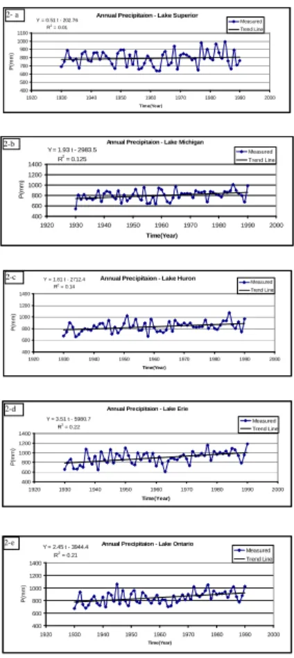
4.1 Historical precipitation trends

Precipitation trend characterization is challenging since precipitation varies

substan-15

tially across space and time, and hence difficult to predict a significant long-term change (Mortsch et al., 2000). Nevertheless technical literature reveals there is evi-dence of increasing trend of precipitation; Mortsch et al. 2000) reported annual pre-cipitation trends for regions of Canada near the Great Lakes region are significantly increasing. As well, Filion (2000) cited that Coulson’s (1997) results indicate a

precipi-20

tation increase of 7–18% in northern British Columbia. The long-term precipitation data (1930–1990) for the individual Great Lakes are plotted as annual precipitation versus time in Fig. 2, “a” through “e”. The slopes of the trend lines are highly significant from both the regression modeling and using the Mann-Kendall statistic and low significance

(10)

HESSD

Full Screen / Esc

for Lake Superior, as summarized in Table 2. These results demonstrate there is suf-ficient evidence to indicate (on the basis of 1930–1990 period) an increasing trend in precipitation on the Great Lakes.

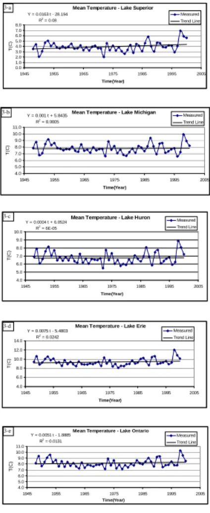
4.2 Trends in temperature

Average annual trends of overlake Temperature versus time (1948–2000), are

illus-5

trated in (Fig. 3 “a” through “e”). The significance of the long-term temperature data for the individual Great Lakes were tested with the results as summarized in the Table 3. None of the trends for temperature were identified as statistically significant at 5% level; the slopes of the regression lines were all positive.

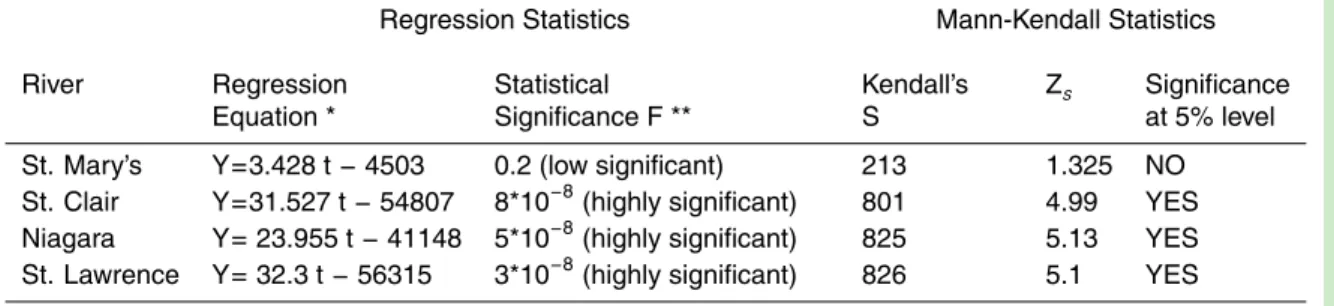
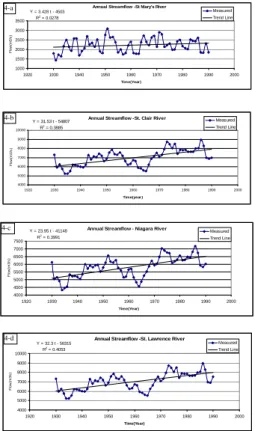
4.3 Trends in measured flows

10

Flow data were analyzed for four locations at various points along the Great Lakes system namely (I) St. Mary’s River, (II) St. Clair River, (III) Niagara River, and (IV) St. Lawrence River, as identified in Fig. 1. These locations represent the sequential locations within the Great Lakes Watershed. The flow magnitudes over time are plotted in Fig. 4 (4-a: St. Mary’s River, 4-b: St. Clair River, 4-c: Niagara River, and 4-d: St.

15

Lawrence River). For 1930–1990, linear regression slopes of the trend lines are highly significant (at 5% level) for all channels except for St. Mary’s River which was low significance. The Mann-Kendall trend test confirms the trend statistics, as summarized in Table 4.

5 Comparison of historical trend projections and GCM predictions

20

If the historical trends continue, the magnitudes of precipitation and flow can be as-sessed for future years, and hence provide a comparison with the projections using the GCMs. It is noted that scenarios of climate change have typically been structured as percent change from the 1960–1990 period, as a means of establishing a baseline

(11)

HESSD

Full Screen / Esc

relative to, for example, the year 2050, the projected year in which there is considered the potential for a doubling of CO₂ in the atmosphere (e.g. after Lofgren et al., 2002). In this context, trend extrapolation of the historical data using the regression equations for each of precipitation, temperatures, and flows, are summarized in Tables 5 through 7, respectively.

5

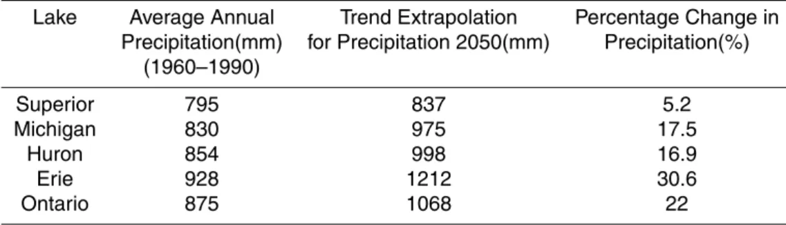
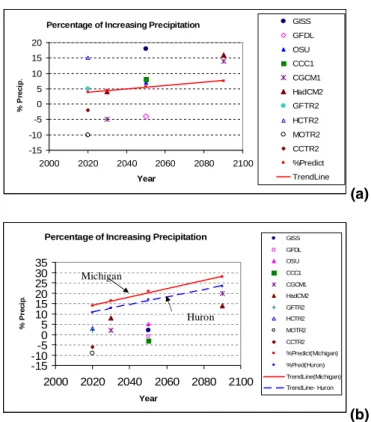
5.1 Prediction of precipitation magnitudes in response to climate change

GCMs are being used to develop future scenarios under changed climate condi-tions (Mortsch et al., 2000). For illustration purposes, the GCM prediccondi-tions for future changes in precipitation for Lake Superior, Lake Michigan and Lake Huron (the latter two combined to Michigan/Huron) from Lofgren (2002) are plotted in Figs. 5(a) and (b).

10

Lofgren et al. (2002) results show that different GCMs produce significantly different predictions; they used outputs from two different types of GCMs namely the equilibrium models (GISS, GFDL, OSU, and CCC1) and the transient models (CGCM1, HadCM2, GFTR2, HCTR2, MOTR2, and CCTR2). The equilibrium models are models that are allowed to run until they reach equilibrium with a predefined atmospheric condition

15

e.g. 2×CO₂. On the contrary, transient models are full dynamic ocean models that are run coupled with an atmosphere with greenhouse content changing with time (Lofgren et al., 2002). In addition to the GCM predictions, also plotted on Figs. 5(a) and (b) are extrapolations using the observed, historical records. As illustrated in Fig. 5(a), for Lake Superior, compared to the prediction by regression, some GCMs overestimate the

20

change in precipitation while some underestimate. For Fig. 5(b), for Michigan/Huron Lakes, the predictions by the regression lines exceed GCM model predictions.

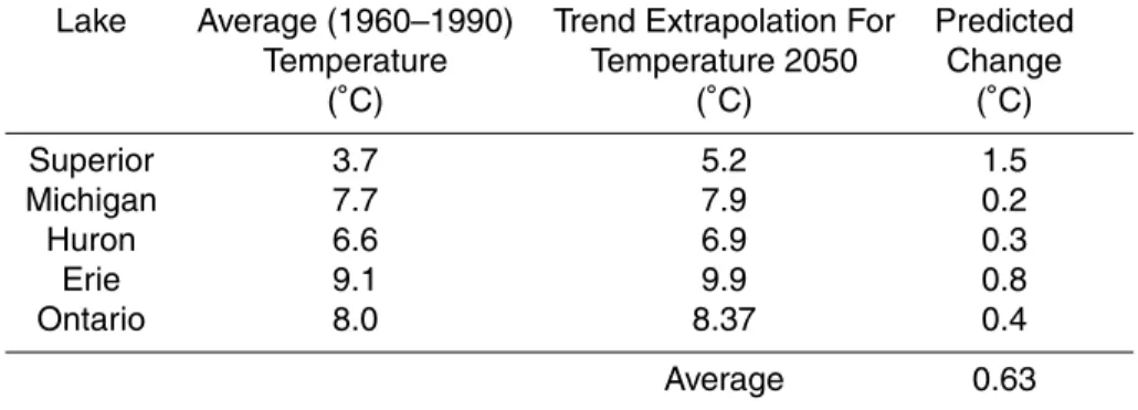
5.2 Prediction of temperature changes to year 2050

According to IPCC, global temperatures are expected to increase by 1.5◦C to 4.5◦C (IPCC, 1996) as opposed to the trend extrapolation of historical data of 0.63◦C (from

25

Table 6). Upon analyzing the data for the period 1895–1999, Mortsch (2000) suggested 3192

(12)

HESSD

Full Screen / Esc

that the annual average temperature for Canada has warmed by a statistically signif-icant 1.3◦C, although the warming is not consistent throughout the time span. The continuation of change in temperature from the observed records can be compared with GCMs’ prediction of future temperature. The GCMs’ predictions are consistently higher than those extrapolated from the historical data as listed in Table 7. Even di

ffer-5

ent GCM predictions are demonstrated as varying amongst themselves by substantial amounts, indicating there are substantial levels of uncertainty associated with temper-ature predictions.

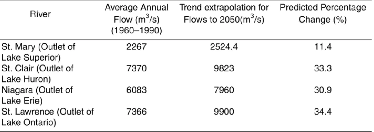
5.3 Prediction of flows to year 2050

The impacts of climate change on water resources are potentially large. Increases

10

in precipitation and temperature could result in dire consequences on water quantity and quality. Precipitation directly translates into runoff, and the regions that experience significant increases in precipitation are likely to have increases in runoff and stream-flows although land use changes may also influence runoff magnitudes. One of the major impacts of climate change would be the changes in frequency and magnitude

15

of extreme hydrologic events (e.g. more intensive rainfall events). Incidence of heavier rainfall events could result in more rapid runoff and greater flooding. As well, heav-ier rainfall may cause deterioration of water quality. Increased rainfall intensity and high magnitude of floods may result in increased erosion of the land surface and the stream channels, higher sediment loads, and increased loadings of nutrient and

con-20

taminants. Based on the observed historical records, annual precipitation rates are significantly increasing over the Great Lakes. This increase in precipitation results in increased streamflows in the Great Lakes system (as apparent from Table 4). The rate of increase in streamflows over the 60 years period (1930–1990) is alarming. From Table 8, the rate of predicted increases in streamflows at the outlet of Lake of

Supe-25

rior, Lake Huron, Lake Erie, and Lake Ontario till 2050 is 11%, 33%, 31%, and 34%, respectively.

(13)

HESSD

Full Screen / Esc

6 Conclusions

Historical records of precipitation, temperature, and streamflows in the Great Lakes system using simple linear regression analysis and non-parametric Mann-Kendall trend test, demonstrate statistically significant increases in precipitation and streaflows over the period 1930–1990. Flow in the St. Mary’s River (outlet of the Lake Superior) shows

5

a gentle increasing trend, whereas flows in the connecting channels at St. Clair River, Niagara River, and St. Lawrence River show statistical significance (at 5% level) trends. Temperature trends were not found to be statistically significant (at 5% level) for any of the five Great Lakes, although the line fitted by regression shows a gentle increasing slope (an increase of 0.63◦C) and less in magnitude than the GCM predictions. The

10

presence of significant positive trends in historical precipitation and flows, and com-parable levels as predicted by the GCMs, indicate that the hydrologic changes being incurred in the Great Lakes system may be attributable to climate change.

Acknowledgements. The assistance from K. Anwar in the assembly of the hydrologic data is

acknowledged.

15

References

Adamowski, K. and Bougadis, J.: “Detection of Trends in Annual Extreme Rainfall”, Hydrol. Process., 17, 3547–3560, 2003.

Beeton, A. M.: “Large Freshwater Lakes: present state, trends, and future”, Environmental Conservation, 29, 21–38, 2002.

20

Boer, G. J., McFarlane, N. A., and Lazare, M.: “Greenhouse Gas-induced Climate Change Simulated with the CCC Second-Generation General Circulation Model”, J. Climate Change, 5, 1045–1077, 1992.

Boer, G. J., Flato, G. M., Reader, M. C., and Ramsden, D.: A transient climate change simula-tion with historical and projected greenhouse gas and aerosol forcing: experimental design

25

and comparison with the instrumental record for the 20th century, Climate Dynamics, 16, 405–425, 2000.

(14)

HESSD

Full Screen / Esc

Printer-friendly Version Interactive Discussion Cohen, S.: “Impacts of C02-induced Climatic Change on Water Resources in the Great Lakes

Basin”, J. Climate Change, 8, 135–153, 1986.

Cohen, S.: “Methodological Issues in Regional Impacts Research”, Proceedings of Confer-ence on Climate Change: Implications for Water and Ecological Resources”, Department of Geography, Occasional Paper No. 11, University of Waterloo, 342, 1990.

5

Croley II, T. E.: “Laurentian Great Lakes Double-CO₂, Climate Change Hydrological Impacts”,

Climatic Change, 17, 27–47, 1990.

Croley II, T. E., Hunter, T. S., and Martin, S. K.: “Great Lakes Monthly Hydrologic Data”, Internal Report, Publications, NOAA, Great Lakes Environmental Research Laboratory, 13, Michigan, USA, 2004.

10

Dulmer, J. M., Pebbles, V., and Gannon, J.: ”North American Great Lakes”, Lake manage-ment initiative regional workshop for Europe, Central Asia and the Americas, Saint Michael’s College, Vermont, USA, 2003.

De Lo ¨e, R. C. and Kreutzwiser, R. D. : “Climate Variability, Climate Change and Water Resource Management in the Great Lakes”, Climatic Change, 45, 163–179, 2000.

15

Filion, Y.: “Climate Change: Implications for Canadian Water Rsources and Hydropower Pro-duction”, Canadian Water Resources Journal, 25, 255–269, 2000.

Gleick, P.: “Methods for Evaluating the Regional Hydrologic Impacts of Global Climatic Changes”, J. Hydrology., 88, 97–116, 1986.

Gleick, P.: “The Development and Testing of a Water Balance Model for Climate Impact

As-20

sessment: Modeling the Sacramento Basin”, Water Resources Research, 23(6), 1049–1061, 1987.

Hansen, J., Russel, G., Rind, D., Stone, P., Lacis, A., Lebedeff, S., Ruedy, R., and Travis,

L.: “Efficient three-dimensional global models for climate studies: Model I and II”, Monthly

Weather Review, 111, 609–662, 1983.

25

Helsel, D. R. and Hirsch, R. M.: “Statistical Methods in Water Resources”, Elsevier Publishers, Amsterdam, Holland, 296–299, 1992.

Hengeveld, H. G.: “Projections for Canada’s climate future: a discussion of recent simulations with the Canadian Global Climate Model”; Environment Canada, Climate Change Digest 00-01, 27 p., 2000.

30

GLIN: “The Great Lakes”, Great Lakes Information Network,http://www.great-lakes.net/lakes,

2005.

IPCC: “Climate Change 1995: The Science of Climate Change.”, Contribution of Working Group

(15)

HESSD

Full Screen / Esc

Printer-friendly Version Interactive Discussion I to the Second Assessment Report of the IPCC, Cambridge University Press, United

King-dom, 1996.

Kendall, M. G.: “Rank Correlation Methods”, 5th Edition, Edward Arnold, 199, London, 1990. Lofgren, B. M., Quinn, F. H., Clites, A. H., Assel, R. A., Eberhardt, A. J., and Luukkonen, C.

L. : “Evaluation of Potential Impacts on Great Lakes Water Resources Based on Climate

5

Scenarios of Two GCMs.”, Journal of Great Lakes Research, 28, 537–554., 2002.

Manabe, S. and Wetherald, B.: “On the distribution of climate change resulting from an increase in CO2 content of the atmosphere”, J. Atmos. Sci., 37, 99–118, 1980.

Mortsch, L., Hengeveld, H., Lister, M., Lofgren, B., Quinn, F., Slivitzky, M., and Wenger, L.: “Cli-mate Change Impacts on the Hydrology of the Great Lakes-St.Lawrence System”, Canadian

10

Water Resources Journal, 25, 153–179, 2000.

Nash, L. L. and Gleick, P.: “The Colorado River Basin and Climate Change: The sensitivity of streamflow and water supply to variations in temperature and precipitation”, EPA, Policy, Planning and Evaluation, EPA 230-R-93-009, 1993.

NOAA: “Hydrology and Hydraulics Data:, National Oceanic and Atmospheric

Administra-15

tion”, Great Lakes Environmental Research Laboratory,http://www.glerl.noaa.gov/data/pgs/

hydrology.html, (visited on 02 May 2005), Michigan, USA, 2004.

Sanderson, M.: “Implications of Climatic Change for Navigation and Power Generation in the Great Lakes”, Climate Change Digest 87-03, Environment Canada, 1987.

Sanderson, M. and Smith, J.: “Climate Change and Water in the Grand; River Basin, Ontario”,

20

Proceedings of the 43rd Conference Canadian Water Resources Association, Penticton, B. C., 243–261, 1990.

Sanderson, M. and Smith, J.: “The Impact of Climate Change on Water in the Grand River Basin, Ontario”, Waterloo, Ontario: Department of Geography, University of Waterloo, 1993.

USEPA: “The Great Lakes” , United States Environmental Protection Agency, (http://www.epa.

25

gov/glnpo/atlas/gl-fact1.html), USA, 2005.

(16)

HESSD

Full Screen / Esc

Table 1. Retention Times for the Great Lakes.

Individual Lake Rank in World(a) Retention Time (years)(b)

by area by volume Superior 2 4 191 Michigan 4 6 99 Huron 5 7 22 Erie 11 – 2.6 Ontario – 12 6

Sources: Beeton (2002)(a)and USEPA (2005)(b).

(17)

HESSD

Full Screen / Esc

Table 2. Statistical trend tests for overlake precipitation versus time.

Regression Statistics Mann-Kendall Statistics Lake Regression Statistical Kendall’s Zs Significance

Equation* Significance F** S at 5% level Superior Y=0.507 t − 202.8 0.43 (low significant) 65 0.404 NO Michigan Y= 1.9031 − 2983 0.005 (highly significant) 440 2.74 YES Huron Y= 1.801 t − 2712 0.0032 (highly significant) 447 2.78 YES Erie Y= 3.509 t − 5981 0.0001 (highly significant) 595 3.7 YES Ontario Y= 2.45 t − 3944 0.0002 (highly significant) 599 3.75 YES

Z_0.025= 1.96

Legend:

* t= Time

** The smaller the F, the more significant the trend. Lesser than 0.01 means highly significance.

(18)

HESSD

Full Screen / Esc

Table 3. Statistical trend tests for temperatures versus time.

Regression Statistics Mann-Kendall Statistics Lake Regression Statistical Kendall’s S Z_s Significance

Equation* Significance F ** at 5% level Superior Y=0.0163 t − 28.194 0.04 (low significant) − 48 0.5 NO Michigan Y= 0.001 t + 5.8435 0.88 (low significant) − 84 0.88 NO Huron Y=0.0004 t + 6.0524 0.95 (low significant) − 136 1.4 NO Erie Y= 0.0075 t − 5.4803 0.26 (low significant) − 78 0.81 NO Ontario Y= 0.0051 t − 1.8885 0.41 (low significant) − 44 0.46 NO

Z_0.025= 1.96

Legend:

* t= Time

** The smaller the F, the more significant the trend. Lesser than 0.01 meanshighly significance.

(19)

HESSD

Full Screen / Esc

Table 4. Results of statistical trend tests for time series of flows in connecting channels.

Regression Statistics Mann-Kendall Statistics River Regression Statistical Kendall’s Zs Significance

Equation * Significance F ** S at 5% level St. Mary’s Y=3.428 t − 4503 0.2 (low significant) 213 1.325 NO St. Clair Y=31.527 t − 54807 8*10−8(highly significant) 801 4.99 YES Niagara Y= 23.955 t − 41148 5*10−8(highly significant) 825 5.13 YES St. Lawrence Y= 32.3 t − 56315 3*10−8(highly significant) 826 5.1 YES

Z_0.025= 1.96

Legend:

* t= Time

** The smaller the F, the more significant the trend. Lesser than 0.01 means highly significance.

(20)

HESSD

Full Screen / Esc

Table 5. Predicted changes in precipitation to 2050 from historical trend projections.

Lake Average Annual Trend Extrapolation Percentage Change in

Precipitation(mm) for Precipitation 2050(mm) Precipitation(%)

(1960–1990) Superior 795 837 5.2 Michigan 830 975 17.5 Huron 854 998 16.9 Erie 928 1212 30.6 Ontario 875 1068 22 3201

(21)

HESSD

Full Screen / Esc

Table 6. Predicted changes in temperatures to 2050 from historical trend projections.

Lake Average (1960–1990) Trend Extrapolation For Predicted

Temperature Temperature 2050 Change

(◦C) (◦C) (◦C) Superior 3.7 5.2 1.5 Michigan 7.7 7.9 0.2 Huron 6.6 6.9 0.3 Erie 9.1 9.9 0.8 Ontario 8.0 8.37 0.4 Average 0.63 3202

(22)

HESSD

Full Screen / Esc

Table 7. Comparison of future temperatures for projections from historical trends and GCMs.

Lake Average Temperature

(◦C) of Base case

(1960–1990)

Projected Temperature (◦C) for 2050

From From GCMs(a)

Historical Trends

projections _GISS _GFDL _OSU

Superior 3.7 5.2 (1.5) 6.6 (2.9) 9.5 (5.8) 5.7 (2.0) Michigan 7.7 7.90 (0.2) 11.9 (4.2) 13.4 (5.7) 10.7 (3.0) Huron 6.6 6.90 (0.3) 9.9 (3.3) 11.7 (5.1) 8.6 (2.0) Erie 9.1 9.9 (0.8) 13.8 (4.7) 14.8 (5.7) 12.5 (3.4) Ontario 8.0 8.37 (0.37) 11.8 (3.8) 13.1 (5.1) 10.4 (2.4) Average 7.02 7.65 (0.63) 10.8 (3.8) 12.5 (5.5) 9.6 (2.6)

Note: values within parentheses represent the change in projected temperature compared to

the Base Case (1960–1990) mean. a= Values extracted from Croley (1990).

(23)

HESSD

Full Screen / Esc

Table 8. Predicted changes in flows to 2050 from historical trend projections.

River Average Annual Trend extrapolation for Predicted Percentage

Flow (m3/s) Flows to 2050(m3/s) Change (%)

(1960–1990) St. Mary (Outlet of 2267 2524.4 11.4 Lake Superior) St. Clair (Outlet of 7370 9823 33.3 Lake Huron) Niagara (Outlet of 6083 7960 30.9 Lake Erie) St. Lawrence (Outlet of 7366 9900 34.4 Lake Ontario) 3204

(24)

HESSD

Full Screen / Esc

Printer-friendly Version Interactive Discussion fig01

Fig. 1. The Great Lakes Basin.

(25)

HESSD

Full Screen / Esc

Annual Precipitaion - Lake Superior

Y = 0.51 t - 202.76 R2 = 0.01 400 500 600 700 800 900 1000 1100 1920 1930 1940 1950 1960 1970 1980 1990 2000 Time(Year) P( m m ) Measured Trend Line 2- a

Annual Precipitaion - Lake Michigan Y = 1.93 t - 2983.5 R2 = 0.125 400 600 800 1000 1200 1400 1920 1930 1940 1950 1960 1970 1980 1990 2000 Time(Year) P (m m) Measured Trend Line 2-b

Annual Precipitaion - Lake Huron

Y = 1.81 t - 2712.4 R2 = 0.14 400 600 800 1000 1200 1400 1920 1930 1940 1950 1960 1970 1980 1990 2000 Time(Year) P( m m) Measured Trend Line 2-c

Annual Precipitaion - Lake Erie

Y = 3.51 t - 5980.7 R2 = 0.22 400 600 800 1000 1200 1400 1920 1930 1940 1950 1960 1970 1980 1990 2000 Time(Year) P (m m) Measured Trend Line 2-d

Annual Precipitaion - Lake Ontario Y = 2.45 t - 3944.4 R2 = 0.21 400 600 800 1000 1200 1400 1920 1930 1940 1950 1960 1970 1980 1990 2000 Time(Year) P( m m) Measured Trend Line 2-e

Fig. 2. (“a” through “e”) – Annual average precipitations versus time.

(26)

HESSD

Full Screen / Esc

Mean Temperature - Lake Superior Y = 0.0163 t - 28.194 R2 = 0.08 0.0 1.0 2.0 3.0 4.0 5.0 6.0 7.0 8.0 1945 1955 1965 1975 1985 1995 2005 Time(Year) T (C) Measured Trend Line 3-a

Mean Temperature - Lake Michigan

Y = 0.001 t + 5.8435 R2 = 0.0005 4.0 5.0 6.0 7.0 8.0 9.0 10.0 11.0 1945 1955 1965 1975 1985 1995 2005 Time(Year) T (C) Measured Trend Line 3-b

Mean Temperature - Lake Huron

Y = 0.0004 t + 6.0524 R2 = 6E-05 4.0 5.0 6.0 7.0 8.0 9.0 10.0 1945 1955 1965 1975 1985 1995 2005 Time(Year) T (C) Measured Trend Line 3-c

Mean Temperature - Lake Erie Y = 0.0075 t - 5.4803 R2 = 0.0242 4.0 6.0 8.0 10.0 12.0 14.0 1945 1955 1965 1975 1985 1995 2005 Time(Year) T (C) Measured Trend Line 3-d

Mean Temperature - Lake Ontario Y = 0.0051 t - 1.8885 R2 = 0.0131 4.0 5.0 6.0 7.0 8.0 9.0 10.0 11.0 1945 1955 1965 1975 1985 1995 2005 Time(Year) T (C) Measured Trend Line 3-e

Fig. 3. (“a” through “e”) – Annual average temperatures versus time.

(27)

HESSD

Full Screen / Esc

Annual Streamflow -St Mary's River Y = 3.428 t - 4503 R2 = 0.0278 1000 1500 2000 2500 3000 3500 1920 1930 1940 1950 1960 1970 1980 1990 2000 Time(Year) F lo w (m 3 /s ) Measured Trend Line 4-a

Annual Streamflow -St. Clair River Y = 31.53 t - 54807 R2 = 0.3885 4000 5000 6000 7000 8000 9000 10000 1920 1930 1940 1950 1960 1970 1980 1990 2000 Time(year) F lo w (m 3 /s) Measured Trend Line 4-b

Annual Streamflow - Niagara River Y = 23.95 t - 41148 R2 = 0.3991 4000 4500 5000 5500 6000 6500 7000 7500 1920 1930 1940 1950 1960 1970 1980 1990 2000 Time(Year) F lo w (m 3 /s) Measured Trend Line 4-c

Annual Streamflow -St. Lawrence River Y = 32.3 t - 56315 R2 = 0.4053 4000 5000 6000 7000 8000 9000 10000 1920 1930 1940 1950 1960 1970 1980 1990 2000 Time(Year) F lo w (m 3/s ) Measured Trend Line 4-d

Fig. 4. (“a” through “d”) – River flows at various locations within the Great Watersheds versus

Time.

(28)

HESSD

Full Screen / Esc

Printer-friendly Version Interactive Discussion Percentage of Increasing Precipitation

-15 -10 -5 0 5 10 15 20 2000 2020 2040 2060 2080 2100 Year % P re c ip. GISS GFDL OSU CCC1 CGCM1 HadCM2 GFTR2 HCTR2 MOTR2 CCTR2 %Predict TrendLine (a) Percentage of Increasing Precipitation

-15 -10 -50 5 10 15 20 25 30 35 2000 2020 2040 2060 2080 2100 Year % P rec ip. GISS GFDL OSU CCC1 CGCM1 HadCM2 GFTR2 HCTR2 MOTR2 CCTR2 %Predict(Michigan) %Pred(Huron) TrendLine(Michigan) TrendLine- Huron Huron Michigan (b)

Fig. 5. (a) Comparison of results of GCMs models by Lofgren et al. (2002) with predicted

model in Lake of Superior.(b) Comparison of results of GCMs models by Lofgren et al. (2002)

with predicted model in Lake Michigan and Lake Huron.