HAL Id: hal-01864373
https://hal.archives-ouvertes.fr/hal-01864373
Submitted on 29 Aug 2018
HAL is a multi-disciplinary open access
archive for the deposit and dissemination of
sci-entific research documents, whether they are
pub-lished or not. The documents may come from
teaching and research institutions in France or
abroad, or from public or private research centers.
L’archive ouverte pluridisciplinaire HAL, est
destinée au dépôt et à la diffusion de documents
scientifiques de niveau recherche, publiés ou non,
émanant des établissements d’enseignement et de
recherche français ou étrangers, des laboratoires
publics ou privés.
by X-ray tomography
Alexis Burr, Clément Ballot, Pierre Lhuissier, Patricia Martinerie, Christophe
L. Martin, Armelle Philip
To cite this version:
Alexis Burr, Clément Ballot, Pierre Lhuissier, Patricia Martinerie, Christophe L. Martin, et al.. Pore
morphology of polar firn around closure revealed by X-ray tomography. The Cryosphere, Copernicus
2018, 12 (7), pp.2481-2500. �10.5194/tc-12-2481-2018�. �hal-01864373�
the Creative Commons Attribution 4.0 License.
Pore morphology of polar firn around closure revealed
by X-ray tomography
Alexis Burr1,2, Clément Ballot1,2, Pierre Lhuissier2, Patricia Martinerie1, Christophe L. Martin2, and Armelle Philip1
1Univ. Grenoble Alpes, Grenoble INP, CNRS, IRD, IGE, 38000 Grenoble, France
2Univ. Grenoble Alpes, CNRS, Grenoble INP, SIMaP, 38000 Grenoble, France
Correspondence: Armelle Philip (armelle.philip@univ-grenoble-alpes.fr) Received: 17 January 2018 – Discussion started: 27 February 2018 Revised: 28 June 2018 – Accepted: 4 July 2018 – Published: 26 July 2018
Abstract. Understanding the slow densification process of polar firn into ice is essential in order to constrain the age difference between the ice matrix and entrapped gases. The progressive microstructure evolution of the firn column with depth leads to pore closure and gas entrapment. Air transport models in the firn usually include a closed porosity profile based on available data. Pycnometry or melting–refreezing techniques have been used to obtain the ratio of closed to to-tal porosity and air content in closed pores, respectively. X-ray-computed tomography is complementary to these meth-ods, as it enables one to obtain the full pore network in 3-D. This study takes advantage of this nondestructive technique to discuss the morphological evolution of pores on four dif-ferent Antarctic sites. The computation of refined geomet-rical parameters for the very cold polar sites Dome C and Lock In (the two Antarctic plateau sites studied here) pro-vides new information that could be used in further studies. The comparison of these two sites shows a more tortuous pore network at Lock In than at Dome C, which should result in older gas ages in deep firn at Lock In. A comprehensive es-timation of the different errors related to X-ray tomography and to the sample variability has been performed. The proce-dure described here may be used as a guideline for further ex-perimental characterization of firn samples. We show that the closed-to-total porosity ratio, which is classically used for the detection of pore closure, is strongly affected by the sample size, the image reconstruction, and spatial heterogeneities. In this work, we introduce an alternative parameter, the connec-tivity index, which is practically independent of sample size and image acquisition conditions, and that accurately pre-dicts the close-off depth and density. Its strength also lies in its simple computation, without any assumption of the pore
status (open or close). The close-off prediction is obtained for Dome C and Lock In, without any further numerical sim-ulations on images (e.g., by permeability or diffusivity cal-culations).
1 Introduction
Ancient atmospheric air is embedded in polar ice caps, mak-ing them a major source of data for reconstructmak-ing past cli-mates (Barnola et al., 1991; Battle et al., 1996). For exam-ple, the EPICA community traced climate variability back to 800 kyr before present (Augustin et al., 2004) from ice cores drilled at Dome Concordia (also named Dome C). The firn layer (approximately the first 50–100 m of the ice cores) is paramount in tackling the reconstruction of past climates, as the gradual densification of snow to ice leads to air entrap-ment. This firnication can last from a few centuries to a few thousand years before pore occlusion, with the consequence that the entrapped air is younger than the surrounding ice at a given depth (Schwander and Stauffer, 1984; Schwander et al., 1988). Unambiguously linking gas composition (from the air) and temperature evolution (from water isotopes in ice) in past climate conditions is challenging. In addition, the progressive closure of pores usually leads to a broad distri-bution of the trace gas ages. Seasonal layering of the polar firn also influences this closure (e.g., Stauffer et al., 1985; Mitchell et al., 2015). In other words, the precise evalua-tion of the gas–ice age difference (1age) requires a detailed understanding of the densification and gas trapping mecha-nisms.
A further complication is that, although the firn under-goes a similar densification with depth until it converts into solid ice, each polar site exhibits peculiar characteristics (lo-cal temperature, accumulation rate, impurity content, topog-raphy, etc.). Thus, climate proxies and air dating strongly de-pend on the polar sites investigated and there is now substan-tial literature that proposes multi-site studies (Landais et al., 2013; Veres et al., 2013; Bazin et al., 2013).
The firn column is classically divided into three distinct zones (Sowers et al., 1992). When considering air circula-tion, a convective zone, where gases are mixed with the at-mosphere in the top layers due to the high permeability of snow and/or the effect of wind, is first encountered. Deeper in the firn, in the diffusive zone, molecular diffusion domi-nates and gravitational fractionation also occurs. The lock-in depth (LID) is defined as the depth at which gravitational fractionation stops (Battle et al., 1996). In the deepest firn zone named the lock-in zone (LIZ), the transport of gases in open pores becomes limited and eventually stops because pores close and entrap air. At the bottom of this zone, the close-off depth (COD) is the depth at which pores are fully isolated from the surface and at which air cannot be pumped out of the firn anymore.
Successive densification mechanisms appear along the firn column. Snow undergoes grain rearrangement, fracture, and sintering until a critical density of 550 kg m−3 is reached (Anderson and Benson, 1963). This density corresponds to an approximate porosity of 40 %, close to the porosity that characterizes a random close pack (RCP) of spheres (Scott and Kilgour, 1969). As for many other granular materials, further densification requires the plastic deformation of the grains themselves. Above 550 kg m−3, dislocation creep be-comes the dominant mechanism for densification (Maeno and Ebinuma, 1983). The last stage of densification is
poros-ity related. When the densporos-ity exceeds about 840 kg m−3,
pores are closed and further shrinking is driven by the differ-ence between their internal pressure and the larger surround-ing stress.
The mechanisms of pore closure in deep firn are of interest in order to understand the relationship between atmospheric signals and trace gas records in firn and ice. Models of gas transport in firn generally include a parameterization of the closed-to-total porosity ratio (e.g., Buizert et al., 2012). How-ever, only a few closed porosity datasets are available (Stauf-fer et al., 1985; Schwander et al., 1993; Trudinger et al., 1997; Gregory et al., 2014; Schaller et al., 2017). Moreover, some recent studies emphasize the effect of firn layering, fur-ther motivating microstructural studies (e.g., Freitag et al., 2013; Gregory et al., 2014; Mitchell et al., 2015; Rhodes et al., 2016; Fourteau et al., 2017).
The ratio of closed to total porosity may be obtained us-ing two different techniques: pycnometry (e.g., Schwander and Stauffer, 1984), and X-ray-computed tomography (e.g., Barnola et al., 2004). Air content measurements are generally performed with melting–refreezing techniques used on
sam-ples taken well below the bubble closure zone and used as a proxy of the average air isolation density (e.g., Martinerie et al., 1992, 1994). Recently, Mitchell et al. (2015) measured air content in the LIZ of the WAIS Divide ice core and used it as an indicator of the bubble closure rate. Each technique comes with its own issues. Air content measurements, when performed on firn samples, may artificially open some closed pores that are weakly sealed and melting–refreezing is a de-structive technique that forbids any further microstructural investigation (Raynaud et al., 1982). Pycnometry only pro-vides a bulk closed porosity value without information on pore morphology. X-ray tomography scans a rather small volume of firn, thus questioning the representativeness of measured properties (Coléou et al., 2001). These three tech-niques all have the issue of border effects in common. In particular, one has to make assumptions on the closed or open status of cut pores. Regarding this issue, the effect of cut pores seems nonetheless much smaller in the case of air content data obtained from bubbles well below the LIZ (e.g., Martinerie et al., 1992, 1994), than in the case of pycnom-etry or closed pores digitized by X-ray tomography on firn samples taken in the LIZ.
The X-ray tomography technique has received increas-ing interest in the last 20 years for investigatincreas-ing snow and firn microstructure (e.g., Flin et al., 2003; Barnola et al., 2004; Schneebeli and Sokratov, 2004; Freitag et al., 2004; Fujita et al., 2009; Lomonaco et al., 2011; Gregory et al., 2014). Focusing on the microstructural evolution that ac-companies the closure process, Barnola et al. (2004) demon-strated the potential of the method by investigating the den-sity and closed poroden-sity evolution along the firn core of Vos-tok. They uncovered significant discrepancies between the ratio of closed porosity calculated from absorption images and measured by pycnometry. They attributed these
differ-ences to the small scanned volumes (0.785 cm3) compared
to those used when performing pycnometry measurements (100 cm3). Fujita et al. (2009) reported that the stratifica-tion of firn has an effect on several properties such as struc-tural anisotropy, crystal orientated fabric, and the total air content at Dome Fuji. Other Antarctic sites (WAIS Divide and Megadunes in East Antarctica) were also investigated. WAIS Divide exhibits a high accumulation rate and relatively warm temperature, whereas Megadunes is very cold, with a very low accumulation rate. Gregory et al. (2014) performed X-ray tomography and permeability measurements on these firn cores. They concluded that the coldest site is charterized by a less tortuous pore morphology. Taking into ac-count the strong layering exhibited in WAIS Divide, Gregory et al. (2014) also proposed that the air flow in polar firn is mainly controlled by pore structure and not so much by den-sity variability. Focusing on the Summit site in Greenland, Lomonaco et al. (2011) closely studied finely grained layers in the firn. Their results indicate that the ratio of the number of closed pores to the pore volume is marked by a sharp in-crease that related well with the LID. Gregory et al. (2014)
also used such a parameter but no relation with the LID can be observed in their Fig. 7. In contrast to this index, the in-crease in the closed-to-total porosity ratio is in better agree-ment with the LID. Overall, the literature on firn tomography concentrates on studying the evolution of structural parame-ters (such as permeability) and their relation to gas transport within the firn. It also focuses on differentiating polar sites, or relating microstructure to deformation mechanisms. How-ever, despite giving useful information for densification mod-eling (e.g., Hörhold et al., 2011, 2012), these X-ray tomog-raphy studies do not provide an unambiguous prediction of LIZ and COD. To that end, the recent work of Schaller et al. (2017) uses X-ray tomography to scan very large volumes of firn from three different polar sites. Their study depicts an abrupt closure of pores when reaching a critical porosity (around 10 %) that is independent of the temperature site.
More generally, for X-ray tomography to become a reli-able reference technique for firn investigation, errors due to acquisition (voxel size or resolution), image analysis (im-age thresholding, labeling of pores), and sample variability (size and spatial heterogeneities) and their impact on the mi-crostructural properties should be thoroughly studied. This effort has already started for modeling based on X-ray to-mography images, whether for physical effective properties (Freitag et al., 2002; Courville et al., 2010) or for snow mechanics (Wautier et al., 2015; Rolland du Roscoat et al., 2007). For example, Freitag et al. (2002) and Courville et al. (2010) modeled the firn permeability with a lattice Boltz-mann technique on a layered firn column using X-ray images. These authors worked out a representative volume element for permeability, going beyond the sole density as performed by Coléou et al. (2001), for example.
In this context, here we investigate in detail the error sources that come with the process of X-ray tomography imaging on two East Antarctica firn cores originating from Dome C and Lock In (located 136 km away from the Con-cordia station towards Dumont d’Urville). We gather several microstructural parameters, such as density, closed-to-total porosity ratio, surface area, and anisotropy, in order to study the closure of pores. We are able to discriminate which pa-rameters correlate to the COD, as defined by the ultimate firn air pumping depth.
The paper is organized as follows. Section 2 details the characteristics of the sites studied here. Section 3 focuses on the errors originating from reconstruction and image pro-cessing of tomographic scans. In Sect. 4, we investigate the scale effect and determine the errors generated for the main physical properties studied when decreasing the resolution in the tomographic scans. Section 5 focuses on the compari-son among four different sites, with particular interest in the two sites studied in this work (namely Dome C and Lock In), along with the polar sites detailed in Gregory et al. (2014). Section 6 takes advantage of image analysis tools to com-pute refined microstructural parameters that characterize the pore network throughout densification.
Two sites in Antarctica are studied, Dome C and Lock In1. Dome C, near Concordia station, exhibits very cold mean
an-nual temperature (−55◦C) and low snow accumulation rate
˙
b(≈ 2.5 cm water equivalent per year, cm yr−1). Moreover, Dome C is at 3233 m a.s.l., with a thickness of nearly 3300 m of ice. These characteristics make it an interesting site for drilling, as it shelters old ice (Augustin et al., 2004). Another distinctive feature of this site is the very narrow non-diffusive zone (LIZ about 3 m; Landais et al., 2006). The ultimate depth reached to sample air by pumping is 99.5 m (Landais et al., 2006; Sturges et al., 2001). The ice cores studied come from the Volsol project carried out in 2010/2011 (Gautier et al., 2016). The firn samples originate from a unique ice core. Three ice samples (115.05, 123.34, and 132.07 m) from the DC12 ice core drilled in 2012 were also analyzed.
The Lock In site is located 136 km away from the Concor-dia station towards the French base Dumont d’Urville. This site was sampled during the austral summer 2015–2016, and is characterized by a higher snow accumulation rate of about
˙
b =4.5 cm yr−1(first guess from Verfaillie et al., 2012). The
borehole temperature is −53.15◦C at 20 m of depth. The
LID is located between 96 and 100 m (Anaïs J. Orsi, personal communication, 2017), and air could not be pumped below approximately 108 m indicating that the COD is deeper than for Dome C. A summary of the different site characteristics is given in Table 1.
3 Methods
3.1 Acquisition parameters
X-ray microcomputed tomography was performed on sam-ples coming from a large range of depths with a refined char-acterization close to the depth at which closure of pores initi-ates. The majority of the samples are labeled S (for small) from Dome C and Lock In, named DC-S12 and LI-S12 (see Table 2 for information on resolution of samples, which varies between 12 and 60 µm). S12 refers to small samples with a voxel side length of 12 µm. These were drilled with a milling machine in slices of ice core such that the cylinder axis is along the core axis (vertical axis). The uncertainty of depth after drilling in slices is estimated to ±0.05 m for all Lock In samples and most Dome C samples (a few sample depths are known at ±0.5 m). Samples were machined down to a diameter of 12 mm with a lathe. The machining opera-tions were performed in a cold room at −10◦C, usually the day before scanning. Scanning geometry was helical in order to image long samples (from 12 to 30 mm) with a volume more than twice the value typically studied by Barnola et al. (2004) and Gregory et al. (2014). Scans were performed at
1Note that Lock In is a polar site and does not refer to the lock-in phenomenon.
Table 1. Characteristics of different polar sites that were studied with X-ray tomography. ˙bdenotes the accumulation rate. The close-off depth is defined as the ultimate depth at which air could be sampled. The lock-in zone is the width between the LID (depth at which gravitational fractionation of δ15N stops) and the COD and is defined as the LIZ width. The temperature is the mean annual temperature or borehole temperature.
Site Location b˙(cm yr−1) hT i(◦C) LIZ width (m) COD (m) Dome Ca,b 75◦60S, 123◦210E 2.5 −55 3 99.5 Lock In 74◦8.3100S, 126◦9.5100E ≈4.5 −53.15 8–12c 108.3 Dome Fujib,d 77◦190S, 39◦400E 2.1 −57 0 104 Vostoka,b,e 77◦280S, 106◦480E 2.2 −57 2 100 WAIS Dividef,g 79◦46.3000S, 112◦12.3170W 21 −31 ≈10 76.5 Megadunesf,h 80◦77.9140S, 124◦48.7960E <4 −49 ≈4 68.5 Summiti,j 72◦34.480N, 37◦38.240W 21 −31 10 80
aBréant et al. (2017).bLandais et al. (2006).cAnaïs J. Orsi (personal communication, 2017).dFujita et al. (2009).eBarnola et al. (2004). fGregory et al. (2014).gBattle et al. (2011).hSeveringhaus et al. (2010).iSchwander et al. (1993).jWitrant et al. (2012).
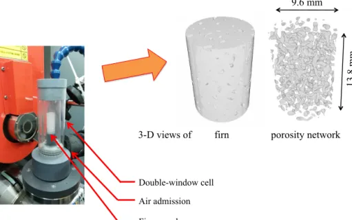
Double-window cell Air admission Firn sample
3-D views of firn porosity network
13.8 m m 9.6 mm
Figure 1. A firn sample from Dome C (100.38 m) inside the cold cell during X-ray tomography imaging, with associated 3-D images of a firn sample and of its pore network.
60 kV with 800 radiographs over four turns leading to a scan time of approximately 25 min per sample. Samples were po-sitioned in a cold cell, cooled by air at −10◦C thanks to the coupling of an air dryer and a cryostat. The temperature was controlled by a thermocouple positioned against the sample holder inside the cell. Schematic of the setup and geometry of the samples are shown in Figs. 1 and 2.
Three samples labeled L (for large) were also charac-terized to investigate the scale effect. They were placed in polystyrene boxes with an eutectic cold pack inside. Sam-ples and cold pack inertia kept the temperature below 0◦C,
ranging from −18◦C to an observed maximum at −3◦C
af-ter 1.5 h (corresponding to two scans). According to meta-morphism experiments of Kaempfer and Schneebeli (2007) and considering the thermal inertia of these large samples,
any microstructural evolution should be negligible during the 1.5 h scanning time. Moreover, two samples were scanned a
first time, kept at −10◦C for 6 months, and then scanned
a second time. No evolution was observed. Volumes M (for medium) were also locally scanned inside the L samples, i.e., a second scan is performed at a higher resolution (using a voxel size of 30 µm instead of 60 µm) and a larger accelera-tion voltage (80 kV instead of 60 kV). Due to the size of the detector, and the position of the cold cell with respect to the X-ray source, there are no M12, L12, or L30 samples that could have been scanned. Sample characteristics are detailed in Table 2 and the extracted volumes are illustrated in Fig. 2.
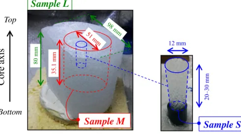
80 m m 20 –3 0 m m 12 mm
Sample L
Sample S
35.1 m mSample M
Core
a
xi
s
Top
Bottom
Figure 2. Schematic of the different sample sizes used in this work. Sample characteristics are listed in Table 2. In green, large samples (L) of the firn core were characterized with X-ray tomography using a voxel side length of 60 µm. Zooming inside the L samples enables us to obtain medium-sized samples (typical of the size used in pycnometry measurements) named M and shown in red. These were scanned at 30 µm (DC-M30). More than 40 samples (shown in blue) of size S were machined separately and scanned at 12 µm for both sites (samples DC-S12 and LI-S12).
Table 2. Three-dimensional image characteristics from Dome C (DC) and Lock In (LI). Samples are scanned with an acceleration voltage of 60 kV except for DC-M30 and DC-S30 volumes, scanned under 80 kV. DC-L60 samples have a polyhedron geometry. M and S volumes are cylindrical. DC-C12 and LI-C12 are cubic (C) subvolumes of DC-S12 and LI-S12, respectively. For DC-L60 to DC-S30, the region of interest (ROI) comes from the same three large samples (L). DC-S12 and DC-C12 come from the same 29 S samples. LI-S12 and LI-C12 come from the same 13 S samples. The number at the end of volume name refers to the voxel size in microns.
Origin Name
Diameter/ ROI Voxel Number
Depth (m) Remarks side (mm) volume size of ROI
of ROI (cm3) (µm) volumes
DC DC-L60 >400 60 3 87.34; 94.5; 100.33 Slice of ice core from Dome C DC DC-M60 51 ≈72 60 3 ” Zoom within the DC-L60
sam-ples
DC DC-M30 51 ≈72 30 3 ” Scans within the L samples DC DC-S30 9.6 1.305 30 39 ” Subvolumes from the DC-M30
samples
DC DC-S12 9.6 0.782–1.781 12 29 22.33–100.38 Cylinders taken from ice core slices
DC DC-C12 6.72 0.303 12 29 ” Cubic subvolumes from the DC-S12 samples
LI LI-S12 9.6 1.303–1.738 12 13 66–120 Samples from Lock In
LI LI-C12 6.72 0.303 12 13 ” Cubic subvolumes from the LI-S12 samples
3.2 Reconstruction and image processing
Reconstruction of the 3-D sample structure is carried out with a filtered-back projection algorithm while image pro-cessing uses the free software Fiji (Schindelin et al., 2012). For S12 samples, a median filter of size 3 is first performed with the plug-in Analysis 3-D developed by Boulos et al. (2013) in order to reduce noise and enhance contrast. The high contrast between air and ice ensures a straightforward
threshold of 3-D binary images. Outliers (persisting noise ar-tifacts) of 2 or 3 voxels were removed, leading to the loss of some micropores with a diameter smaller than 36 µm. This represents less than 0.7 % of the total porosity and leads to an estimated 0.1 % error for density.
A cylindrical region of interest (ROI) is systematically ex-tracted from the digitized sample to ensure that the analysis is not perturbed by ice fragments localized on the sample borders (typically originating from machining). Pore
label-ing is also performed on this ROI uslabel-ing the Analysis 3D plug-in (Boulos et al., 2013). All extracted ROIs are de-tailed in Table 2. The errors introduced successively by the potential sublimation of matter inside the cell during scan-ning time, the reconstruction, and the image processing (fil-tering and thresholding) were determined as follows. On a smaller sample height (h = 12 mm), tomographic scans last-ing 5 min were repeated durlast-ing 3 h on a 86 m deep sample from Dome C, first, every 5 min, then with increasing in-tervals of time. The results for these 12 scans have shown that sublimation was limited to the outward 0.2 mm of the cylindrical sample after 30 min, even for a porosity for which percolation is significant. As borders are eliminated after extraction of the ROI (diameter of 9.6 mm for S samples with a diameter of 12 mm), there is no influence of the dry air circulation around the firn in the cold cell. Multi-ple acquisitions of the same samMulti-ple allow a global error to be computed. This includes errors from acquisition proce-dure, image reconstruction and Fiji processing (median fil-ter + thresholding + outliers removal).
Several firn properties such as the density, the specific sur-face area (SSA), and other pore-related parameters are de-termined in this work. The SSA is defined as the surface of the pores over the total sample volume. The surface is computed with the marching cube algorithm (Lorensen and Cline, 1987). The SSA is used to quantify the air–ice inter-actions (e.g., to compute the snow-to-atmosphere flux of ad-sorbed molecules on snow; Domine et al., 2008) or to work out the grain size of firn cores (Linow et al., 2012). The vol-ume used to compute total porosity is calculated by counting voxels. The closed-to-total porosity ratio and the connectivity index (the ratio of the volume of the largest pore to the total pore volume) are also systematically calculated. We charac-terize a closed pore as a pore that does not touch the border of the ROI at the sample resolution. The pore volume fraction is defined as the closed-to-total porosity ratio (as a percentage). Results for these parameters are discussed in Sect. 4.
The 12 successive scans of the same sample are used to compute standard deviations. At 86 m of depth, absolute
er-rors are 1.2 kg m−3 for density, 0.008 mm−1 for the SSA,
0.068 % for the connectivity index, and 0.25 % for the closed porosity ratio, while relative standard errors are respectively 0.15 %, 0.81 %, 0.11 %, and 3.1 %. Since this procedure was performed on only one sample, we assume that the relative errors associated with each microstructural parameter are the same for all depths. In other words, we assume that the pre-cision (from X-ray scans and image processing) for a given property is independent of depth for all S12 samples.
4 Representativeness of morphological parameters
Conducting a refined X-ray characterization and comparison of polar firn requires a correct estimation of possible errors. In addition to precision, several other sources of errors exist
which do not have the same influence on the results. These er-rors can come from spatial heterogeneity, size of the ROI, im-age resolution, imim-age processing, and labeling assumptions.
This section focuses on giving estimates of these errors for the important parameters studied: the density, the closed porosity ratio, the connectivity index, and the SSA. These er-rors depend on depth, except for the numerical ones from re-construction and image processing for which we assume an independent relative value. Results presented hereafter can be useful for future tomographic studies that should advanta-geously include error and variability estimations.
4.1 Density
Densities were determined directly from binary images using ρice=917 kg m−3and are shown against depth for both sites
in Fig. 3a. We also attempted to measure density by weight-ing samples as carried out in Gregory et al. (2014). However, we observed that this method led to a very large dispersion, which may be linked to a too small sample volume. In any case, we chose to link the density measurement directly to the local scanned volume. We believe that this is preferable to ascribing a density originating from a much larger volume as carried out by Gregory et al. (2014), which may not be representative of the actual scanned sample.
Figure 3a illustrates the increase in density with depth. It also shows that for a given depth, the density at Dome C is larger than at Lock In. As stated above, the relative error in measuring density is less than 0.15 % and thus is not shown here. For approximately the same depth, differences between the density of Dome C and Lock In samples are between 1.8 and 2.6 % (in the range of depths studied).
The density of Dome C samples obtained with X-ray to-mography superimposes correctly with the scattered data of Leduc-Leballeur et al. (2015), who worked out density by measuring the mass and volume of samples 5 cm long. The high-resolution density measurements performed by Leduc-Leballeur et al. (2015) required a large number of samples (30 to 37 samples in every 2 m layer), thus explaining the observed scattering in their measurements.
Densification of firn into ice leads to a transition at which an open pore, which enabled air to flow, begins to separate into different pores. This closure of pores occurs all along the firn core but is more pronounced just before the close-off,
typically when density ranges between 800 and 840 kg m−3
where we gathered more data points. Figure 3b is a zoom-in on this region for Dome C. A mean density profile was proposed at Dome C (Bréant et al., 2017) and goes below
80 m, with a standard deviation of 6.2 kg m−3. While
DC-S12 densities and the density profile [Bre2017] seem in ac-cordance before 85 m in Fig. 3a, they diverge deeper in the firn in Fig. 3b, with DC-S12 densities being above the density profile and its standard deviation. Except for samples from 94.5 m, calculating the density from a binary image seems to overestimate the mean density by approximately 2 % in
Figure 3. (a) Evolution of density with depth for Dome C and Lock In. (b) Zoom-in from (a) focused on Dome C for various ROI sizes (S, M, L) and voxel sizes (12, 30, and 60 µm). Box plots contain data from DC-S30 volumes. Hereafter, boxes represent lower and upper quartiles, the black lines inside being the median values. The confidence interval is set to account for all the data (no outliers). Green dots [Led2015] in (a) are data obtained by Leduc-Leballeur et al. (2015) from volume and mass measurements of 5 cm thick samples from a Dome C ice core down to 80 m. The blue dashed line [Bre2017] corresponds to a mean density profile of Dome C averaged on a 25 cm scale from Bréant et al. (2017). The blue shaded area in (b) represents a standard deviation of 6.2 kg m−3between the fit and density data as given by Bréant et al. (2017).
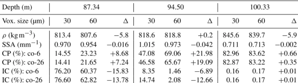
Table 3. Results and differences between DC-M30 and M60 samples. Results with 6 and 26 connected voxels are shown.
Depth (m) 87.34 94.50 100.33 Vox. size (µm) 30 60 1 30 60 1 30 60 1 ρ(kg m−3) 813.4 807.6 −5.8 818.6 818.8 +0.2 845.6 839.7 −5.9 SSA (mm−1) 0.970 0.954 −0.016 1.015 0.973 −0.042 0.711 0.713 −0.002 CP (%): co-6 14.55 23.23 +8.68 47.08 69.06 +21.98 82.96 83.62 +0.66 CP (%): co-26 14.41 21.65 +7.24 46.58 65.67 +19.09 82.87 83.22 +0.35 IC (%): co-6 76.20 60.37 −15.83 8.35 1.46 −6.89 0.16 0.17 +0.01 IC (%): co-26 76.60 62.82 −13.78 14.74 2.08 −12.66 0.16 0.17 +0.01
the 85–100 m range. Three DC-S12 samples were extracted from the same slice of ice core at 86, 91, and 98 m of depth. These triplets of points are barely distinguishable. The red box plots shown in this figure represent the extrema on 13 subvolume measurements (small DC-S30 images) originat-ing from a medium-sized DC-M30 sample. These box plots show dispersion inside medium-sized samples (subvolumes of 1.3 cm3inside 72 cm3). The difference between the maxi-mal and minimaxi-mal values for samples from the same depth is less than 2.5 % (maximum variability is obtained at 94.5 m). Thus, the effects of spatial heterogeneities and of the size of the ROI are limited but are the main contributions to the variability in the density. Indeed, three additional S samples were scanned at a voxel side length of 12 and 30 µm and ex-hibited differences of less than 0.1 % for density. Similarly, the difference between densities of the samples DC-M30 and DC-M60 is less than 1 % (see Table 3). The layered nature of polar firn has already been studied and discussed in the lit-erature (Hörhold et al., 2011; Freitag et al., 2013), and could be detected using X-ray scanning (Freitag et al., 2013; Gre-gory et al., 2014). Very cold polar sites such as Dome C with
low accumulation usually exhibit limited layering (Landais et al., 2006); however, the recent work of Fourteau et al. (2017) does show layering at the centimeter scale for the low-accumulation sites of Vostok and Dome C. Our sample shape and discontinuous measurements do not allow us to discuss such anomalies in polar firn. In conclusion, according to the relatively low variability among samples in terms of density, DC-S12 samples are large enough to estimate the density of a slice of firn of the same height within 2.5 % errors.
4.2 Closed porosity
The closed-to-total porosity ratio (CP) is obtained by divid-ing the total volume of closed pores (VCP) in the ROI by the
total volume of pores (Vpores):
CP = VCP
Vpores
. (1)
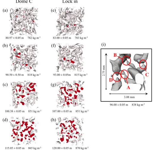
Figure 4 shows the evolution of closed pores (in red) within the firn pore network for Dome C and Lock In. The number of closed pores increases with depth, and separation
(a) (e) (b) (f) (c) (g) (d) (h)
Dome C
Lock in
93.00 ± 0.05m 815 kg m-3 90.50 ± 0.50 m 818 kg m-3 80.97 ± 0.05 m 782 kg m-3 83.00 ± 0.05 m 783 kg m-3 100.38 ± 0.05 m 851 kg m-3 107.00 ± 0.05 m 851 kg m-3 115.05 ± 0.05 m 865 kg m-3 120.00 ± 0.05 m 870 kg m-3 3.08 mm 2.75 m mA
B
C
D
96.00 ± 0.05 m 838 kg m-3 (i)Figure 4. Evolution of closed pores (red) within the firn porosity network (grey) for different depths at Dome C and Lock In sites for DC-C12 and LI-C12 volumes (cross-section dimension is 6.72 × 6.72 mm2). Note that (a, e), (b, f), (c, g), and (d, h) have approximately the same density. (i) Close-up view from a DC-C12 volume of a few channels among pores at different stages of the pinching process illustrated by areas A, B, C, and D.
persists even for pores already closed. We observed that the separation of pores arises by pinching of the channel link-ing two larger globular portions of the pore as illustrated by Fig. 4i. Areas A and B in Fig. 4i show examples of channels on the verge of disappearing, while areas C and D highlight newly pinched pores (dead ends).
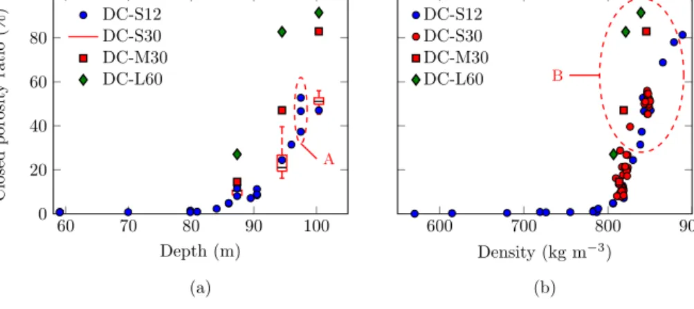
Figure 5a shows a steep increase in the closed porosity ratio for DC-S12 samples, starting at 80 m of depth (corre-sponding to approximately 780 kg m−3). As in Fig. 3b, at 86, 91, and 98 m of depth, three DC-S12 samples were extracted from the same slice of ice core to evaluate dispersion (area A in Fig. 5a). The DC-S30 volumes are represented by box plots, which are rather large (especially at 94.5 m of depth). Boxes represent lower and upper quartiles of the distribution of the closed porosity ratio, with the median value in black. The confidence intervals take into account all data points. Spatial heterogeneities in the closed porosity ratio strongly depend on depth. This variability among small volumes is particularly pronounced at 94.5 and 98 m, but smaller when closed pores are few (at 87.34 m) or after the COD as defined
by the last firn air pumping depth (sample from 100.33 m, whereas the COD is at 99.5 m; Landais et al., 2006; Witrant et al., 2012). This leaves two possibilities. First, the firn may be very heterogeneous horizontally, meaning that a single DC-S12 sample is not representative enough for the closed porosity ratio of the firn for this particular depth. Second, it could mean that our definition of a closed pore is not appro-priate, due to the sample boundary conditions. Note that for such depths (94.5 and 98 m), the mean size of a closed pore is still likely too large to hold inside the DC-S12 samples.
ROI size also has a strong influence on the estimation of the closed porosity ratio. Indeed, the larger the volume, the larger the closed porosity ratio (Fig. 5). Note that this effect is more pronounced at 100.33 m (compare volumes DC-M30 and DC-S12) than at 87.34 m of depth. Errors due to coars-ening in resolution are summarized in Table 3 and reveal a significant effect on the results between the DC-M30 and DC-M60 volumes2. The closed porosity ratio is always larger
2DC-M60 and DC-M30 have the same ROI, but are scanned for a voxel side length of 30 and 60 µm respectively (see Table 2)
Figure 5. Evolution of the closed porosity as a percentage of total porosity against (a) depth and (b) density for various sample sizes (S, M, L) and voxel sizes (12, 30, and 60 µm). The variability in the closed porosity of various samples from the same depth is represented by red box plots in (a) and red dots in (b) as densities are not exactly identical.
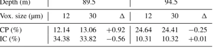
when increasing the voxel size, and this effect is similar to the one of the ROI volume. For labeling, the type of connectivity (6 or 26) is also investigated, and its influence on the results is limited for all resolutions considered. Using 26 connected voxels does enhance the possibility for different pores to be more connected than it is with only 6 connected voxels as cu-bic voxels are not only connected through faces (6) but also through edges and corners (26). It is especially true at the depths of 87.34 and 94.5 m as this is where pinching is very pronounced and on the verge of cutting pore channels. Thus a change in the definition of the pores as implied by the use of 26 connected voxels might connect some closed pores to-gether or to the surface. Similarly, coarsening the resolution means a different threshold value when segmenting the im-age and thus a possible separation of pores or channels. This seems to be especially true for low resolution, e.g., here for a voxel size of 60 µm. Indeed, differences related to voxel size between the same volumes DC-S12 and DC-S30 are smaller, as the relative error for the closed porosity ratio is less than 7 % with respect to the 12 µm resolution (see Table 4). This is relatively low compared to the extent of the box plot rep-resented in Fig. 5a, which spans from 16 to 40 % at 94.5 m of depth.
All the samples and the subvolumes extracted are plotted versus density in Fig. 5b. While the smallest volumes seem to follow a trend, the largest ones are still spread (area B in Fig. 5b). From this plot it is impossible to determine at which density or closed porosity ratio the close-off could be unambiguously identified. Considering air content in firn, the parameterization from Goujon et al. (2003) assumes that the volume fraction of closed pores is approximately 37 % at the average air isolation level (defined as the average porous vol-ume or density of air isolation calculated from air content measurements; Martinerie et al., 1992, 1994). Conversely, at 94.5 m of depth DC-M30 and DC-L60 volumes showed that 47 % to 82 % of pores are closed at 94.5 m of depth, for
ex-ample. Such high values could suggest that the close-off oc-curs at a shallower depth than commonly accepted. However, the density of this sample (ρ = 821 kg m−3) is lower than the average air isolation density obtained by Martinerie et al. (1992) (ρ = 840 kg m−3), and air was pumped out of the firn down to 99.5 m (Landais et al., 2006), which is 5 m below the DC-L60 sample taken at 94.5 m of depth. Additionally, the rather large voxel size leads to separation of pores that are linked by channels the diameter of which is below the image resolution, artificially increasing the closed porosity ratio.
Therefore, the rather large errors for the closed porosity ratio of DC-L60 samples call for caution in interpreting re-sults (see Table 3). In short, the most appropriate use of the closed porosity ratio requires large volumes associated with high resolutions.
4.3 Connectivity index
In this section, we propose an alternative indicator of the pore closure, which is much less sensitive to the source of errors that characterize the closed porosity ratio, especially the sam-ple size. The connectivity index (CI) is defined by the ratio between the volume of the largest pore (Vlargest_pore) and the
total volume of pores (Vpores):
CI =Vlargest_pore Vpores
. (2)
It was originally introduced by Babin et al. (2006) to de-pict void coalescence in bread. It proved useful (under the name “interlinkage parameter”) in quantifying the coales-cence of cavities during superplastic deformation of an alu-minum alloy (Martin et al., 2000), or as a criterion to op-timize box sizes when smoothing density maps of graphite with inclusions (Babout et al., 2006). The evolution of the connectivity index leads to pertinent information on the per-colation process of pores, as it describes how the largest pore
Figure 6. Evolution of the connectivity index (volume of the largest pore divided by total pore volume) with (a) depth and (b) density. The variability in the connectivity index of various samples from the same depth is represented by red box plots in (a) and red dots in (b) as the densities are not exactly identical.
evolves with the drop in the total pore volume. It tends to 0 when all pores are separated and/or shrinking. The trend is paramount for connectivity index interpretation, as fluctu-ations could mean unusual change in pore size distribution. Contrary to the closed porosity ratio, the connectivity index is independent of sample boundary conditions since all pores are considered. This is critical for small volumes as the ratio of surface to volume becomes significant. However, it is very dependent on the statistical size of pores and their number inside the samples.
As shown in Fig. 6, the connectivity index is maximum and close to 100 % when the porosity is totally open (one large pore overcomes all others; the pore network is almost fully interconnected), while it is very small (less than 0.2 %; see Table 3) when all pores are closed. The connectivity
in-dex drops around 780 kg m−3 (≈ 80 m) and stagnates after
850 kg m−3 (100 m). Subsampling leads to large box plots
and thus large variability at 87.34 and 94.5 m, while it is much smaller at 100.33 m. Thus spatial heterogeneity is pro-nounced during the drop in the connectivity index. DC-M30 or DC-L60 volumes are inside or close to the box plot. This is in contrast with the closed porosity ratio in Fig. 5 in which DC-M30 or DC-L60 volumes are far from the box plot. This means that the use of the connectivity index induces a much weaker effect of the ROI volume. Comparing resolution and type of connectivity of the DC-S12 and DC-S30 volumes, results for the connectivity index are similar to the closed porosity ratio (differences of less than 7 % in Table 4). Ta-ble 3 also lists errors between the DC-M30 and DC-M60 vol-umes for the connectivity index. Overall, these ROIs fall in the box plots of the DC-S30 volumes (see Fig. 6a).
In conclusion, the variability in the connectivity index comes mostly from the horizontal spatial heterogeneity. It is much less sensitive to the volume of the samples, the resolu-tion, or the type of connected voxels than the closed porosity ratio. Interestingly, Fig. 6b indicates that the connectivity in-dex points fall on a master curve when plotted against the
density. In particular, a clear drop in the connectivity index is observed at a density of about 830 kg m−3. Above this den-sity, DC-L60 and DC-M30 exhibit no large pores anymore. At Dome C, the last firn air pumping depth is 99.5 m (Landais et al., 2006) and Martinerie et al. (1992) obtained a density of 840 kg m−3at average air isolation level from air content measurements. Thus, according to Fig. 6, the connectivity in-dex is a good predictor of the close-off. However, it does not give any information on the LID, which is required for 1age estimation.
4.4 Specific surface area
The SSA involves the quantification of the surface of the pores. This measurement is voxel size dependent due to the surface roughness. However, as shown by Tables 3–5, dif-ferences of voxel size do not lead to too large of an error. Changes due to ROI volume and connectivities are also not significant for the SSA. These results are very similar to those obtained for density; however, the effect of the spatial heterogeneity is more pronounced. Indeed, in the worst case scenario, relative differences for the same depth can reach up to 20 %. All the other sources of errors give results in the range of the variability in the horizontal spatial hetero-geneities. Also, all data points are known very precisely as pores are defined by a large number of voxels. In the fol-lowing, the surface-area-to-volume ratio is used instead of the SSA for comparison with Gregory et al. (2014). Both pa-rameters mostly reflect the pore surface. However the vol-ume considered for the surface-area-to-volvol-ume ratio is the porous phase instead of the whole ROI. The relative standard error for the surface-area-to-volume ratio (S/V ) is 0.47 % (Table 5).
4.5 Key results on error estimations
To sum up, in this section we have separately characterized the errors associated with the calculated microstructural
pa-Depth (m) 89.5 94.5 Vox. size (µm) 12 30 1 12 30 1 CP (%) 12.14 13.06 +0.92 24.64 24.41 −0.25 IC (%) 34.38 33.82 −0.56 10.31 10.32 +0.01
Table 5. Absolute and relative errors for two DC-S12 samples. Rel-ative errors are determined thanks to Sect. 3.2.
Depth (m) 84.07 Abs. err. 97.5 Abs. err. Rel. err. ρ(kg m−3) 788.4 ±1.2 841.5 ±1.3 0.15 % SSA (mm−1) 1.192 ±0.010 0.750 ±0.006 0.81 % S/V (mm−1) 8.478 ±0.040 9.108 ±0.043 0.47 % CP (%): co-6 2.32 ±0.07 52.74 ±1.63 3.1 % CP (%): co-26 2.32 ±0.07 52.03 ±1.61 3.1 % IC (%): co-6 88.654 ±0.098 2.883 ±0.003 0.11 % IC (%): co-26 88.654 ±0.098 2.883 ±0.003 0.11 %
rameters when choosing the resolution, the type of connected voxels, and the size of the sample. Table 3 and Figs. 5 and 6 showed that the variability in the results can be signifi-cant and is dependent on the depth of the sample. The closed porosity ratio was shown to be dependent on ROI size, voxel size, and spatial heterogeneities. When plotted versus den-sity, the connectivity index is revealed to be a very appropri-ate parameter to describe the progressive pore closure. The proposed connectivity index is a more discriminant parame-ter to describe the pore closure, as it is foremost dependent on spatial heterogeneities.
The precise determination of microstructural parameters requires a small voxel size. With X-ray tomography, this means a small sample volume. Therefore, in the following, only samples whose voxel side length is 12 µm are studied and compared. In order to avoid overloading the following figures, uncertainties are not displayed but Table 5 allows the absolute uncertainties for two distinct depths of the DC-S12 samples to be reported.
5 Multi-site comparisons
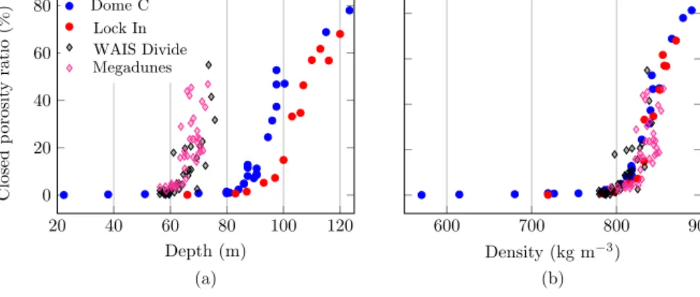
In this section, we compare our data retrieved from Dome C and Lock In to those originating from WAIS Divide (West Antarctica) and Megadunes (East Antarctica) from Gregory et al. (2014), which were also analyzed with X-ray tomog-raphy. We focus on the closed porosity ratio and morpho-logical parameters that can be compared for all four sites. We note however that the depth intervals probed for the WAIS Divide and Megadunes sites are smaller than ours. Temperature and accumulation conditions for WAIS Divide and Megadunes are listed in Table 1; porosity closes at a much shallower depth, between 60 and 80 m for WAIS Di-vide and Megadunes, as indicated by Fig. 7a, than Dome C
and Lock In. In contrast, pore closure occurs below 80 m for Dome C and Lock In. The Lock In site has a larger accu-mulation rate and is a bit warmer than Dome C but exhibits a deeper closure of pores. When plotting the percentage of closed porosity against density, Fig. 7b shows that all points fall approximately on a master curve. This supports the idea that the close-off arises on first approximation at a particular density. Note that the Megadunes site is peculiar, as a dune experiences continuous snow deposition on its sides and has an average of zero accumulation in “hiatus” zones (Courville et al., 2007; Severinghaus et al., 2010).
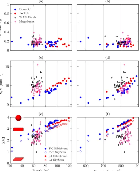
Figure 8 shows three morphological parameters of interest (degree of anisotropy, surface-area-to-volume ratio of pores, and structure model index (SMI)) that can be compared for all four sites. The evolution of these parameters is shown against depth (Fig. 8a, c, e) and against density (Fig. 8b, d, f). These geometrical parameters provide valuable information on the pore network morphology that could be useful for the understanding of firnification.
Figure 8a, b show the degree of anisotropy that was deter-mined using the BoneJ plug-in (Doube et al., 2010) on the pore phase. This parameter is calculated using a 3-D mean intercept length method that directly works out all possi-ble directions. An ellipsoid is fitted to the scaled intercepted points, giving eigenvalues for the lengths of the ellipsoid axes. The degree of anisotropy of the morphology is 0 for a fully isotropic structure and tends to unity when all objects are aligned along a direction. Figure 8a, b indicate that for all four sites, the degree of anisotropy is rather low (≤ 0.4), with a mean value on the order of 0.2. No clear trend is observable with depth or density.
The surface-area-to-volume ratio (S/V ) of the pores is de-picted in Fig. 8c, d. S/V may be seen as a good descriptor of the complexity of the pore network morphology. In the case of pores as shown in Fig. 4, pore roughness is similar for both sites (pore surfaces are smooth). Therefore, a less tortu-ous network leads to a smaller S/V value. In contrast with anisotropy (Fig. 8a, b) a clear difference is observable be-tween Dome C and Lock In sites on the one hand and WAIS Divide and Megadunes sites on the other hand. Our data in-dicate a fairly smooth trend for the Dome C and Lock In sites, whereas the WAIS Divide and Megadunes sites (Gre-gory et al., 2014) show much more variability on a rather lim-ited depth interval. Gregory et al. (2014) characterized sam-ples from both finely grained and coarsely grained layers. The microstructural differences that inherently come with fine and coarse grains should explain the variability observed in their results. Concentrating on the S/V ratio against den-sity (Fig. 8d), and focusing on the limited common denden-sity
interval (750–850 kg m−3), we note that WAIS Divide
ex-hibits the most tortuous pore network. The Megadunes site leads to a pore network the S/V values of which are in be-tween those of Dome C and Lock In, but again with a much larger variability. Although relatively limited, there is a clear difference between Dome C and Lock In, with Dome C
con-Figure 7. Comparison among four polar sites – Dome C, Lock In, WAIS Divide, and Megadunes – of the closed porosity evolution with (a) depth and (b) density. Diamonds are data points from Gregory et al. (2014).
sistently exhibiting smaller S/V values than Lock In, either for the same density or for the same depth. Thus, Lock In presents, for a given depth or density, a more tortuous pore network than Dome C. Dome C and Lock In S/V values fol-low approximately a linear increase with depth.
The structure model index (SMI) is a popular index in the bone research community which is implemented in the SkyScan software CT-analyzer (http://bruker-microct.com, last access: 19 July 2018) used by Gregory et al. (2014). It was also used to analyze snow metamorphism for instance (Schneebeli and Sokratov, 2004; Kaempfer and Schneebeli, 2007). The SMI describes the shape of pores, with positive values for convex shapes and negative values for concave ones. The SMI tends to 0 for plates, 3 for rods, and 4 for spherical particles. Two different methods are available to compute the SMI: the SkyScan plug-in and the BoneJ plug-in with the Hildebrand algorithms (Hildebrand and Rüegsegger, 1997). As highlighted by Salmon et al. (2015), the SkyScan plug-in consistently leads to smaller SMI values than the Hildebrand plug-in. For the sake of comparison with the data of Gregory et al. (2014), Fig. 8e, f show the structure model index (SMI) of the porous phase obtained with both meth-ods. As for the SSA, the SMI is computed using the pore surface area. Consequently, uncertainties are negligible and not shown.
As for the S/V parameter, the SMI computed by Gre-gory et al. (2014) (using the SkyScan plug-in) exhibits a much larger variability than ours. In other words, the pore shapes measured at WAIS Divide range from semicylindri-cal to nearly spherisemicylindri-cal for a rather limited span of depth (55– 70 m) or density. In contrast, data points from Dome C and Lock In follow a clear trend, which suggests a simple evolu-tion from rod-like to sphere-like shape for increasing depth or density.
We have checked that the difference between WAIS Divide and Megadunes on the one hand and Dome C and Lock In data on the other hand does not originate from the different methodologies used in the two groups by computing the SMI
of Dome C and Lock In with the same plug-in used for WAIS Divide and Megadunes. As shown by Fig. 8e, f, the SkyScan plug-in leads indeed to smaller SMI values than Hildebrand algorithms. But this does not contradict the general picture that Dome C – Lock In and WAIS Divide – Megadunes sites differ markedly when considering the morphology of pores. In any case, we believe that the linear evolution observed in Fig. 8e, f for Dome C and Lock In is pertinent as it relates well with the change in pore morphology shown in Fig. 4.
6 Refined geometrical parameters for Dome C and
Lock In sites
In the preceding section, we have compared four different sites using available data from the literature. In this sec-tion, we take advantage of the collected 3-D images for Dome C and Lock In to compute refined geometrical param-eters. They should bring new insights into the intimate struc-ture of firn and its evolution, and are also useful properties that can be used for diffusion or permeability modeling.
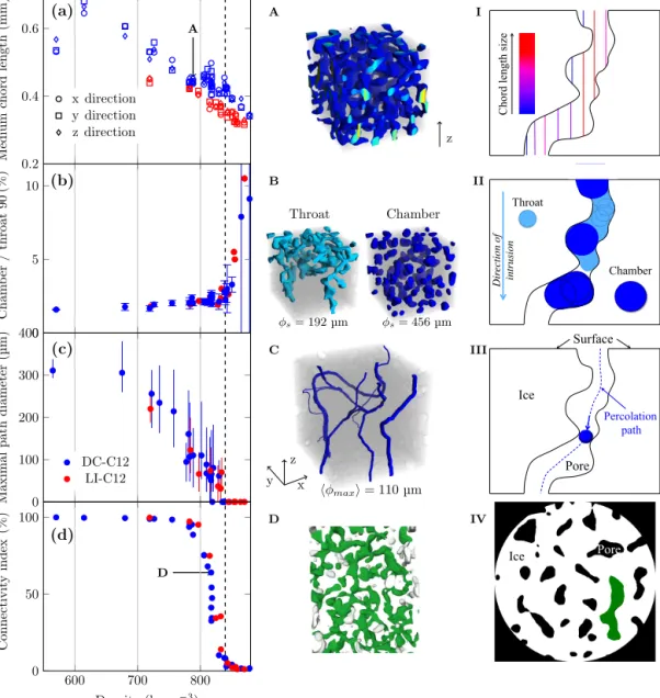
We have chosen to plot these parameters as a function of density alone but their evolution against depth can be ob-tained by fitting the data points in Fig. 3. Figure 9 sums up and defines these parameters: medium chord length (Fig. 9a), chamber-to-throat size ratio (Fig. 9b), maximal path diam-eter (Fig. 9c), and connectivity index defined in Sect. 4.3 (Fig. 9d). The parameters in Fig. 9a–c have been obtained by using the commercial software GeoDict (https://www. math2market.de/, last access: 19 July 2018). Definitions of these parameters are given hereafter. Volumes DC-C12 and LI-C12 were used, as the software requires parallelepiped ROIs.
Figure 9a shows the medium chord length in all three di-rections. The corresponding sketch only illustrates the in-tercepts in the z direction. The intercept lengths are mea-sured and averaged for each direction. For each density, the medium chord length can be considered isotropic because no
Figure 8. Anisotropy (a, b), surface-area-to-volume ratio (c, d), and structure model index (e, f) plotted against depth and density for Dome C and Lock In (this work) as well as for WAIS Divide and Megadunes (Gregory et al., 2014). The SMI for Dome C and Lock In is computed using both the Hildebrand method (Hildebrand and Rüegsegger, 1997) and the SkyScan plug-in.
preferential direction can be determined. Both DC-C12 and LI-C12 depict a linear decrease of about 50 % from 22.33 to 100.38 m of depth for Dome C. For a given density, the medium chord length of LI-C12 is always smaller than that of the DC-C12 volumes. This confirms the more complex shape of pore morphology for Lock In as observed in Fig. 8. As for the S/V ratio (Fig. 8c, d), we note for Dome C a slight discontinuity of the medium chord length decrease with density at approximately 800 kg m−3. At this density, the medium chord length ceases to decrease. This disconti-nuity is difficult to interpret but may be linked to the pinch-ing of the thinnest channels that arises at the start of the pore closure.
Figure 9b illustrates the ratio of the calculated chamber to throat pore size distribution for the 90th centile. Chamber pore size distribution is worked out using the granulometry over the whole sample, and the throat pore size distribution is obtained here by porosimetry on all sample faces, in the
X, Y , and Z directions. Figure 9, images B and II clarify the throat and chamber concepts (Sweeney and Martin, 2003). The porosimetry consists of the introduction of a sphere from the top surface, thus mimicking the intrusion of liquid from the specimen surface. Each tested size of spheres in the sam-ple is associated with the volume fraction covered by the set of spheres. In Fig. 9II, this is represented by a light blue area in which a particular sphere can circulate. When the space between pores is too small the sphere cannot move down any-more. This is different from the chamber pore size distribu-tion, which is only based on the geometry of pores. Spheres of different sizes are placed in every available space of the porous network in that case. We chose to display the dis-tribution at the 90th centile, as the porosimetry is difficult to perform for a deep sample. This provides the general trend in the closure of pores by pinching while still having large glob-ular parts. Error bars show the standard deviations from the mean value of the porosimetry results on the six cubic faces.
Chord l engt h s iz e Throat Chamber D ir e c ti on of int rus ion Ice Pore Percolation path Surface Ice Pore
Figure 9. Variations with density in (a) the medium chord length, (b) the ratio of chamber size to throat size distribution at the 90th centile, (c) the maximal path diameter, and (d) the connectivity index. The black dashed line is the average air isolation density (ρ = 840 kg m−3) from Martinerie et al. (1992) for Dome C. Three-dimensional images illustrate each parameter on the left-hand side in images A–D. Images A–C come from the same DC-C12 volume at 85 m of depth, while image D is a picture of a 91 m deep volume. φsis the diameter of the sphere which is used for visualization of porosimetry and granulometry. hφmaxiis the mean of the maximum diameter for the different percolation paths. The last column (I–IV) sketches the calculation of parameters.
These are shown only for Dome C. After the air isolation density, there is a drastic increase in this ratio, as pinching reduces the throat size.
Percolation paths on subvolumes were calculated in the zdirection alone. They are evaluated by moving the largest possible sphere inside the pore network, from the top sur-face to the bottom one. For each sample, 10 percolation paths were calculated, starting with a minimum path diameter of 24 µm and then increasing it by 24 µm steps. Figure 9c shows the calculated maximal path diameters. The vertical lines represent the variability based on all paths that are
differ-ent, and the dots are the mean of those maximum diameters. A general decrease is observed, from approximately 300 µm at 550 kg m−3 to zero (i.e., less than 24 µm when reaching approximately 830 kg m−3), which is slightly lower than the air isolation density (840 kg m−3; Martinerie et al., 1992). Again, there are no noticeable differences between Dome C and Lock In. Both sites exhibit a large variability in the max-imal path diameter that can vary between 0 and 200 µm in the same sample. However, these diameters are quantitative information for the path of air (in a given interval). A notice-able issue of this calculation is that the maximal path
diame-Figure 10. Connectivity index for Dome C and Lock In. Vertical solid lines represent the COD defined by the last firn air pump-ing depths in Table 1. Vertical dashed lines correspond to the air isolation depth for temperature of Dome C (−55◦C) and Lock In (−53.15◦C) calculated with the Goujon et al. (2003) parameteriza-tion of the air-content-related close-off density, and using the den-sity profile with depth given in Fig. 3. Black dashed, dotted lines are linear slopes of the connectivity index obtained using a least-square method.
ter depends on the size of the chosen subvolume. Here a cube of 6.72 mm in size was used, which ensures percolation until 830 kg m−3according to Fig. 9. The length of the path ranges from 8 to 18 mm, meaning a tortuous structure whatever the depth. This is shown in image A in Fig. 9. A larger cube would have led to a drop in the maximum path diameter to 0 before 830 kg m−3because of the structural isotropy of the pore network and the erratic process of closure. A smaller porosity amount is associated with a smaller probability of having a network connecting two opposite sample sides. Fig-ure 9b, c do not allow for a clear differentiation between the DC-C12 and LI-C12 samples.
It is instructive to compare the evolution of the connectiv-ity index in Fig. 9d to that of the chamber / throat and max-imal path diameter (Fig. 9b–c). The air isolation density ob-tained by Martinerie et al. (1992) for Dome C is well corre-lated to the end of the drop of the connectivity index (black dashed line). It also correctly separates the two regimes ob-served in Fig. 9b, c.
Figure 10 compares the evolution of the connectivity in-dex with depth for Dome C and Lock In. When the connec-tivity index drops to very small values, Fig. 10 clearly shows a sharp change in the slope for the two sites. As for Fig. 9d, three stages can be clearly distinguished with two horizontal parts and an abrupt linear drop. The last two linear portions of the curve intersect at depths that are in good agreement with both the ultimate depth at which air could be sampled and with the Goujon et al. (2003) parameterization of air iso-lation depth related to air content data of Martinerie et al.
Dome C Lock In 100.38 m 107.00 m Core a xi s
(a)
(b)
Figure 11. Comparison for the same density (ρ = 851 kg m−3) of (a) Dome C and (b) Lock In microstructures as observed with po-larized light. Both thin sections are taken parallel to the core axis.
(1992, 1994). The parameterization is used for temperatures of Dome C and Lock In.
Indeed, the blue and red solid lines correspond to the ulti-mate air pumping depths at Dome C (99.5 m) and Lock In (108.3 m) (see Table 1), whereas the blue and red dashed lines correspond to the parameterization of the air isolation density related to air content measurements, called close-off density in Goujon et al. (2003). The air isolation depth was calculated from our measurements of density (Fig. 3). Us-ing the connectivity index evolution thus seems a promis-ing method to locate the depth and density at which pores are nearly fully closed. Its main advantage is that it does not depend on assumptions or arbitrary choices on the status of pores (closed or open). According to Fig. 10, the end of the connectivity index drop down at Lock In is approximately 8 m below the one of Dome C, consistent with the difference in last firn air sampling depths between these sites.
Although exhibiting a size distribution, grain size mea-surements showed a larger mean grain size at Dome C than at Lock In. Near the close-off depths of Dome C (100 m) and Lock In (108 m), the mean cross-sectional area was measured from thin sections to be approximately 1.78 and 0.59 mm2, respectively. We observed that grains in the Dome C firn
increased in size with depth (from 0.57 mm2 at 60 m to
1.78 mm2at 100 m) while grains in the Lock In firn showed no clear increase in size in the probed depth range (60– 120 m). Figure 11 compares two thin sections of firn from Dome C and Lock In for the same density. This illustrates the clear difference in grain size between these two sites. This in-formation on grain size, together with that on medium chord
length (Fig. 9) and surface-area-to-volume ratio (Fig. 8), sug-gest a more tortuous pore structure for Lock In.
7 Concluding remarks
X-ray characterization of firn samples was performed for two polar sites, Dome C and Lock In, over a broad depth range. We focus on the microstructural markers that accompany the closure of pores. The most obvious method to characterize pore closure is to measure the ratio of closed to total poros-ity. However, building on a thorough estimation of the re-sults’ accuracy after imaging and processing, we have shown that this approach has serious drawbacks as the percentage of closed porosity exhibits large variability with sample size and voxel size and spatial heterogeneities when characterized by X-ray tomography. This is problematic since most models of air transport in the firn such as Battle et al. (2011), Witrant et al. (2012), Buizert et al. (2012), and Trudinger et al. (2013) rely on a diffusion coefficient that requires the knowledge of the evolution of the closed porosity with depth and/or density. Thus, these models depend on a correct parameterization of the volume fraction of closed pores and there is no consensus on those that have been proposed (Schwander, 1989; Goujon et al., 2003; Severinghaus and Battle, 2006; Mitchell et al., 2015; Schaller et al., 2017). The cut-pore effect (Martinerie et al., 1990) also has to be taken into account on the bound-aries of the sample.
Here, we have encountered similar difficulties in unam-biguously determining the fraction of closed pores. For ex-ample, we have determined that near the critical density of 840 kg m−3, it ranges from approximately 20 to 80 %. This uncertainty results from the conjunction of three detrimental effects: the sample size, the voxel size (resolution), and an inherent spatial heterogeneity.
We propose an alternative parameter: the connectivity in-dex, which is simply the volume of the largest pore divided by the total pore volume. The main advantage of the con-nectivity index is that it is much less sensitive to cut pores that undermine the measure of the closed porosity ratio. Be-fore the close-off depth (COD), the connectivity index is es-sentially affected by horizontal spatial heterogeneities in the sample but not much by resolution and sample size. When focusing on the determination of the COD, we have shown that a sample size on the order of 1–2 cm3 is a reasonable choice for the connectivity index determination. In these con-ditions, the connectivity index accurately predicts the COD as defined by the ultimate air sampling depth for the Dome C and Lock In sites. It also agrees with the parameterization of Goujon et al. (2003) related to the air content measure-ments from Martinerie et al. (1992, 1994). When using to-mographic data, we propose using the connectivity index to precisely determine the COD.
That being said, the two sites studied in this work (Dome C and Lock In) are both characterized by cold temperatures
and low accumulation rates. It would be interesting to use the connectivity index at other polar sites to confirm its rel-evance for COD determination. Indeed, further challenging this index at polar sites exhibiting layering such as WAIS Di-vide would help in determining if this metric is appropriate to characterize closure.
In comparison to our work, Schaller et al. (2017) took advantage of X-ray scans on slices 4 cm in height and of the full core diameter to determine the status of subvolume pores (closed or opened). Section 4 discussed the effects of the voxel size by comparing results from samples using 12 and 30 µm. The difference for the closed porosity ratio was less than 7 %. Therefore, results obtained by Schaller et al. (2017) with a voxel size of 25 µm should not be too viti-ated by voxel-relviti-ated errors. However, their definition of a closed pore still necessitates the knowledge of the status of the surrounding pores. This requires having access to larger volumes than those studied. In our work, only three sam-ples have the diameter of the core. In addition, as detailed in Sect. 4, the voxel size of the largest samples has a great in-fluence on the fraction of closed pores. The large samples and voxel size used by Schaller et al. (2017) seem appropriate to reasonably limit cut-pore effect without suffering too much from voxel size issues. However, it is still hindered by the unavoidable possibility of having a large closed pore (larger than the sample) that is wrongly considered open. The use of the connectivity index avoids these issues.
The morphology of pores was compared to data from Gregory et al. (2014) for polar sites WAIS Divide and Megadunes. Their data show more variability than ours, which can be explained by the selection of finely and coarsely grained layers and the different nature of the studied sites. Indeed, Dome C and Lock In are very cold sites with low accumulation, with Dome C at the tip of the dome. In contrast, Megadunes is a site exposed to strong winds that redeposit snow from one side of the dune to the other, thus leading to a non-steady-state site. WAIS Divide is a warmer site with a high accumulation rate. Layering is significant, and high-density layers of fine grains can be found above low-density layers of coarse grains. As Gregory et al. (2014) intentionally extracted samples both from coarsely and finely grained layers, and plotted their data indiscriminately with bulk density, these led to more dispersed results. Using a lo-cal density (density of the scanned sample rather than the density of the whole sample) as done here could have re-duced the dispersion of their results as discussed by Mitchell et al. (2015). Such a strategy could have helped confirm or re-ject that close-off occurs at a critical density as suggested by Schaller et al. (2017), while current inaccurate estimations do not allow such a claim. Again, we believe that the con-nectivity index would clearly answer this question and would discriminate the role of the density and of the microstructure on closure if all curves fall on a master curve.
The polar sites Dome C and Lock In were extensively compared. Shapes of pores, closed porosity, and connectivity