Vertical distribution of chlorophyll a concentration and phytoplankton community composition from in situ fluorescence profiles: a first database for the global ocean

HAL Id: hal-01277176

https://hal.sorbonne-universite.fr/hal-01277176

Submitted on 22 Feb 2016

HAL is a multi-disciplinary open access

archive for the deposit and dissemination of

sci-entific research documents, whether they are

pub-lished or not. The documents may come from

teaching and research institutions in France or

abroad, or from public or private research centers.

L’archive ouverte pluridisciplinaire HAL, est

destinée au dépôt et à la diffusion de documents

scientifiques de niveau recherche, publiés ou non,

émanant des établissements d’enseignement et de

recherche français ou étrangers, des laboratoires

publics ou privés.

phytoplankton community composition from in situ

fluorescence profiles: a first database for the global ocean

R. Sauzède, H. Lavigne, Hervé Claustre, J. Uitz, C. Schmechtig, F.

d’Ortenzio, C. Guinet, S. Pesant

To cite this version:

R. Sauzède, H. Lavigne, Hervé Claustre, J. Uitz, C. Schmechtig, et al.. Vertical distribution of

chloro-phyll a concentration and phytoplankton community composition from in situ fluorescence profiles: a

first database for the global ocean. Earth System Science Data, Copernicus Publications, 2015, 7 (2),

pp.261-273. �10.5194/essd-7-261-2015�. �hal-01277176�

www.earth-syst-sci-data.net/7/261/2015/ doi:10.5194/essd-7-261-2015

© Author(s) 2015. CC Attribution 3.0 License.

Vertical distribution of chlorophyll

a

concentration and

phytoplankton community composition from in situ

fluorescence profiles: a first database for the global

ocean

R. Sauzède1,2, H. Lavigne3, H. Claustre1,2, J. Uitz1,2, C. Schmechtig1,2, F. D’Ortenzio1,2, C. Guinet4, and S. Pesant5,6

1_{Laboratoire d’Océanographie de Villefranche, CNRS, UMR7093, Villefranche-Sur-Mer, France} 2_{Université Pierre et Marie Curie-Paris 6, UMR7093, Laboratoire d’océanographie de Villefranche,}

Villefranche-Sur-Mer, France

3_{Istituto Nazionale di Oceanografia e di Geofisica Sperimentale, Sgonico (OGS), Italy} 4_{Centre d’Etudes Biologiques de Chizé, CNRS, Villiers en Bois, France}

5_{MARUM, Center for Marine Environmental Sciences, Universität Bremen, Bremen, Germany} 6_{PANGAEA, Data Publisher for Earth and Environmental Science, Bremen, Germany}

Correspondence to: R. Sauzède (sauzede@obs-vlfr.fr)

Received: 29 March 2015 – Published in Earth Syst. Sci. Data Discuss.: 21 April 2015 Revised: 31 August 2015 – Accepted: 18 September 2015 – Published: 5 October 2015

Abstract. In vivo chlorophyll a fluorescence is a proxy of chlorophyll a concentration, and is one of the most frequently measured biogeochemical properties in the ocean. Thousands of profiles are available from historical databases and the integration of fluorescence sensors to autonomous platforms has led to a significant increase of chlorophyll fluorescence profile acquisition. To our knowledge, this important source of environmental data has not yet been included in global analyses. A total of 268 127 chlorophyll fluorescence profiles from several databases as well as published and unpublished individual sources were compiled. Following a robust quality control procedure detailed in the present paper, about 49 000 chlorophyll fluorescence profiles were converted into phytoplankton biomass (i.e., chlorophyll a concentration) and size-based community composition (i.e., mi-crophytoplankton, nanophytoplankton and picophytoplankton), using a method specifically developed to har-monize fluorescence profiles from diverse sources. The data span over 5 decades from 1958 to 2015, including observations from all major oceanic basins and all seasons, and depths ranging from the surface to a median maximum sampling depth of around 700 m. Global maps of chlorophyll a concentration and phytoplankton community composition are presented here for the first time. Monthly climatologies were computed for three of Longhurst’s ecological provinces in order to exemplify the potential use of the data product. Original data sets (raw fluorescence profiles) as well as calibrated profiles of phytoplankton biomass and community composition are available on open access at PANGAEA, Data Publisher for Earth and Environmental Science.

Raw fluorescence profiles: http://doi.pangaea.de/10.1594/PANGAEA.844212 and

1 Introduction

Phytoplankton biomass is generally recognized to play a key role in the global carbon cycle, stressing the need for a bet-ter understanding of its spatio-temporal distribution and vari-ability in the global ocean. Chlorophyll a concentration is widely used as a proxy to estimate phytoplankton biomass. The geographic and temporal distribution of this proxy is already well documented at a global scale thanks to syn-optic remote sensing observations by ocean-color radiom-etry (OCR, McClain, 2009; Siegel et al., 2013). Neverthe-less, OCR observations are restricted to the ocean surface layer, “sensing” only one-fifth of the so-called euphotic layer where phytoplankton photosynthesis is realized and which can sometimes extend to well below 100 m (Gordon and Mc-Cluney, 1975; Morel and Berthon, 1989). It is therefore es-sential to better resolve the global distribution of phytoplank-ton biomass in the vertical.

The vertical distribution of chlorophyll a can be estimated with greatest accuracy from the analysis of water samples by high-performance liquid chromatography (HPLC, Claus-tre et al., 2004; Peloquin et al., 2013). However, these in situ measurements are relatively scarce because their ac-quisition requires ship-based sampling and their analysis is costly. Moreover, because these measurements are made on water samples, the vertical resolution is generally weak (e.g., around one measurement every 10 m). The measure-ment of in vivo chlorophyll a fluorescence is widely used as a proxy for chlorophyll a concentration (Lorenzen, 1966). Besides dissolved oxygen concentration, fluorescence is the most measured biogeochemical property in the global ocean. The advantages of this method are as follows: (1) it can be easily measured in situ using reliable sensors; (2) the vertical resolution is high, yielding several values per me-ter; and (3) data are available in digital format immediately after their acquisition. The integration of fluorescence sen-sors on autonomous platforms (e.g., profiling floats, animals, gliders) has recently led to a sudden rise in the acquisition of in vivo chlorophyll a fluorescence data (Claustre et al., 2010a). However, the relationship between chlorophyll a flu-orescence and phytoplankton biomass is highly variable and depends on several factors, including phytoplankton phys-iological state and community composition (Cunningham, 1996; Falkowski et al., 1985; Kiefer, 1973). The conversion of in situ chlorophyll a fluorescence measurements into phy-toplankton biomass must therefore be done with great care.

FLAVOR (Fluorescence to Algal communities Vertical distribution in the Oceanic Realm) is a method developed to transform and combine large numbers of fluorescence pro-files from various sampling sensors and platforms (Sauzède et al., 2015a). This neural network-based method generates vertical distributions of (1) chlorophyll a concentration and (2) phytoplankton community size indices (i.e., microphyto-plankton, nanophytoplankton and picophytoplankton) based on the shape of in situ fluorescence profiles (i.e., normalized

profiles) and the day and location of acquisition. In addition to chlorophyll a concentration, community composition is an essential variable that determines the possible impact of phytoplankton on oceanic carbon fluxes and climate change scenarios (e.g., Le Quere et al., 2005). Global data compi-lations of phytoplankton community composition from dis-crete water samples have recently been published in ESSD (Peloquin et al., 2013) but data remain rather sparse. It could be an invaluable source of information to have a database of phytoplankton community size indices with the same spatio-temporal resolution as the fluorescence data sets. It has now become possible using the FLAVOR method to transform and combine all available in situ fluorescence data into a single-reference database that comprises essential informa-tion on chlorophyll a concentrainforma-tion and phytoplankton com-munity size indices vertical distributions.

Presently, the widely used climatology of the global ver-tical distribution of chlorophyll a concentration is published in the World Ocean Atlas 2001 (Conkright et al., 2002). The latter climatology is based on estimates from analyzed water samples available in the World Ocean Database (WOD, Lev-itus et al., 2013) and the World Data Center (WDC, http:// gcmd.gsfc.nasa.gov/). This climatology, based on seven dis-crete depths (0-10-20-30-50-75-100 m), is mainly limited by the lack of in situ estimations of chlorophyll a concentration, which leads to a strong spatial interpolation of data. More-over, the discrete depths used to compute the climatology fail to finely reproduce the vertical distribution of the phyto-plankton biomass, especially in areas characterized by very deep (> 100 m) deep chlorophyll maxima (DCM) such as the core of subtropical oligotrophic gyres. Using FLAVOR, the potential of the high vertical (around one data point per me-ter) and spatial resolution of chlorophyll fluorescence mea-surements would improve the 3-D climatologies of chloro-phyll a concentration significantly. Moreover, climatologies of phytoplankton community size indices could be created with a similar spatio-temporal resolution.

This paper presents a global compilation of chlorophyll fluorescence profiles obtained from online databases and from published and unpublished individual sources. These were converted into a global compilation of phytoplankton biomass (i.e., chlorophyll a concentration) and community composition using the FLAVOR method. Prior to the ap-plication of FLAVOR, a 10-step quality control procedure was specifically developed. The remaining profiles were then analyzed. As examples of application, we present the first maps of global mean chlorophyll a concentration for sev-eral oceanic layers as well as global maps of phytoplank-ton community size indices. To further assess the quality of the resulting database, the climatological chlorophyll a con-centration computed here for the surface layer is compared to the climatological remotely sensed chlorophyll a concen-tration available from Modis Aqua. Moreover, monthly 3-D climatologies of chlorophyll a concentration and associ-ated phytoplankton community size indices are analyzed for

Table 1.Summary of the contributions of the chlorophyll fluorescence profiles in the database presented in this study. Data

source/institute/investigator

Period Number of fluores-cence profiles

Percentage of data in the database

Website if available or contact for requests

National Oceano-graphic Data Center (NODC)

Jun 1958–Mar 2014 30 977 63.7 % http://www.nodc.noaa.gov/

Oceanographic Autonomous Obser-vations (OAO)

May 2008–Jan 2015 6092 12.5 % http://www.oao.obs-vlfr.fr/

Laboratoire d’Océanographie de Villefranche (LOV) cruises

May 1991–Jan 2012 3320 6.8 % claustre@obs-vlfr.fr, sauzede@obs-vlfr.fr

Japan Oceanographic Data Center (JODC)

Jan 1998–Jul 2004 2262 4.6 % http://www.jodc.go.jp/ PANGAEA Nov 1980–Apr 2009 2294 4.7 % http://www.pangaea.de/ C. Guinet (data

ac-quired by elephant seals, Guinet et al., 2013)

Dec 2007–Jan 2011 1908 3.9 % christophe.guinet@cebc.cnrs.fr,

British Oceano-graphic Data Center (BODC)

Sep 1996–Nov 2008 1219 2.5 % http://www.bodc.ac.uk/

Systèmes d’Informations Scientifiques pour la MER (SISMER)

Sep 1999–May 2008 237 0.5 % http://www.ifremer.fr/sismer/

Australian Antarctic Data Center (AADC)

Jan 2001–Feb 2006 234 0.5 % http://data.aad.gov.au/ Southern Ocean Iron

RElease Experiment (SOIREE)

Feb 1999 57 0.1 % http://www.uea.ac.uk/~e610/soiree/index.html

several ecological provinces defined by Longhurst (2010). Overall, the data set presented here can be readily exploited to deepen our understanding of the spatio-temporal distribu-tion and variability of phytoplankton biomass and associated community composition in the global ocean. It is obviously a first step towards a database that will regularly be improved thanks to the ongoing intensification of chlorophyll a fluores-cence profile acquisition by Bio-Argo profiling floats, gliders and mammals equipped with instruments.

2 Data and methods

2.1 Origins of in situ chlorophyll fluorescence measurements

The database presented in this study is available from PAN-GAEA, Data Publisher for Earth and Environmental Science in two formats: (1) the database containing all compiled raw fluorescence profiles (the raw database, http://doi.pangaea. de/10.1594/PANGAEA.844212, Sauzède et al., 2015b) and (2) the database containing the fluorescence profiles which

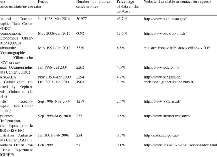
are calibrated into chlorophyll a concentration and as-sociated phytoplankton community size indices (the cali-brated database, http://doi.pangaea.de/10.1594/PANGAEA. 844485, Sauzède et al., 2015c). The data of in situ vertical fluorescence profiles compiled for creating the raw database were obtained from several available online databases as well as published and unpublished individual sources. The dupli-cates and single-surface values, which are not vertical pro-files, were automatically removed (not integrated in the raw database). Finally, the raw database contains 268 127 flu-orescence profiles. Following a robust quality control pro-cedure detailed hereafter (Sect. 2.2), about 49 000 chloro-phyll fluorescence profiles were converted into phytoplank-ton biomass (i.e., chlorophyll a concentration) and size-based community composition (i.e., microphytoplankton, nanophytoplankton and picophytoplankton). The origin of this calibrated database is summarized in Table 1. The ma-jority of the data come from the National Oceanographic Data Center (NODC) and the fluorescence profiles acquired by Bio-Argo floats are available on the Oceanographic Autonomous Observations (OAO) web platform (63.7 and

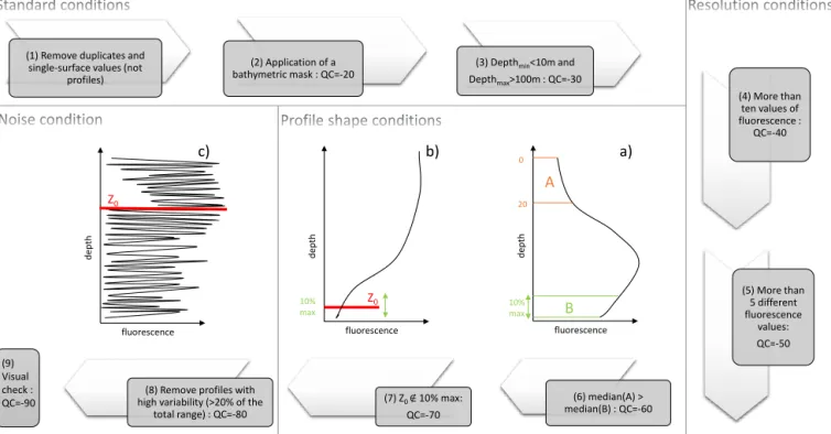
(1) Remove duplicates and single-surface values (not

profiles)

(2) Application of a

bathymetric mask : QC=-20 _Depth(3) Depthmin<10m and

max>100m : QC=-30 (4) More than ten values of fluorescence : QC=-40 (5) More than 5 different fluorescence values: QC=-50 (7) Z0 ∉ 10% max: QC=-70 (6) median(A) > median(B) : QC=-60 (8) Remove profiles with

high variability (>20% of the total range) : QC=-80 (9) Visual check : QC=-90 A B fluorescence d epth 20 0 10% max a) fluorescence d epth 10% max Z0 b) fluorescence d epth Z₀ c)

Figure 1.Schematic overview of the quality control procedure specifically developed for the database presented in this study. The fluores-cence profiles represented in the (a), (b) and (c) panels are examples of profiles which are rejected by the quality control steps (6), (7) and (8) respectively.

12.5 % respectively, see percentages of data in the database depending on their origin in Table 1).

Different modes of acquisition were used to collect the data presented in this study: (1) the CTD (conductivity, tem-perature and depth) profiles are acquired using a fluorometer mounted on a CTD rosette; (2) the OSD (Ocean Station Data) profiles are derived from water samples analyzed by fluorom-etry and are defined as “low” resolution profiles (Boyer et al., 2009); (3) the UOR (Undulating Oceanographic Recorder) profiles are acquired by a “fish” equipped with fluorometer and towed by a research vessel; (4) AP (Autonomous Plat-forms) profiles are acquired by Bio-Argo profiling floats or elephant seals equipped with a fluorometer (Claustre et al., 2010b; Guinet et al., 2013). Table 2 lists the number of pro-files in the calibrated database according to these four modes of acquisition.

It is worth noting that the data acquired from gliders were not included in the database. Although glider data are ex-tremely numerous, they are restricted to a very small spatio-temporal window. As a consequence, a database including glider data would likely be spatially and temporally biased, in contradiction with our first aim of building a global clima-tological database.

Table 2.Summary of the chlorophyll fluorescence profiles in the database presented in the study depending on the different modes of data acquisition.

Acquisition Number of Percentage of data fluorescence profiles in the database

CTD 27 433 56.4 % OSD 10 831 22.3 % UOR 2952 6 % AP 7384 15.2 % Total 48 600 2.2 Quality control

In order to use the FLAVOR method (see details in Sect. 2.3), a specific and adapted data quality control procedure was de-veloped and applied to each in situ chlorophyll fluorescence profile. This procedure was schematically implemented ac-cording to four main steps of data control (Fig. 1), each step being developed for discarding most, if not all, spurious flu-orescence profiles that would deteriorate the quality of the database. Firstly, several basic tests were applied: (1) dupli-cates and single-surface values, which are not vertical pro-files, were removed (these profiles were removed from the beginning of the process so they are not included in the so-called raw database); (2) coastal profiles were removed using

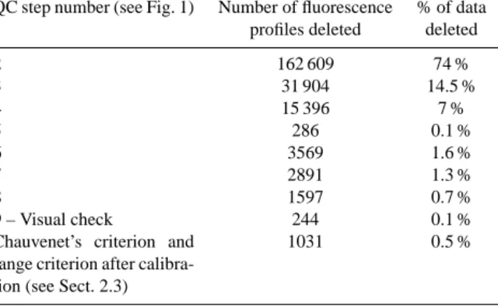
Table 3.Summary of the number of fluorescence profiles rejected at each step of quality control.

QC step number (see Fig. 1) Number of fluorescence % of data profiles deleted deleted

2 162 609 74 % 3 31 904 14.5 % 4 15 396 7 % 5 286 0.1 % 6 3569 1.6 % 7 2891 1.3 % 8 1597 0.7 % 9 – Visual check 244 0.1 %

Chauvenet’s criterion and range criterion after calibra-tion (see Sect. 2.3)

1031 0.5 %

a bathymetric mask of 500 m depth; (3) the uppermost mea-surement has to be located within the 0–10 m layer, while the deepest measurement has to be at or below 100 m. Sec-ondly, tests on the profile vertical resolution are applied: (4) a minimum of 10 values per profile is required (i.e., condition on the vertical resolution acquisition); (5) a minimum of five non-equal values per profile are required (i.e., condition on the sensor resolution). Then, several tests are applied on the fluorescence profile shape. These conditions are based on the parameter used for the development of the FLAVOR method,

Z0, which is the depth at which the fluorescence profile re-turns to a constant background value (see details in Sect. 2.3 and examples in Fig. 1b and c). (6) The median of the fluores-cence values from the surface down to 20 m has to be greater than the median of the values of the last 10 % of the deepest samples of the profile (see Fig. 1a); (7) the depth Z0has not to be within the last 10 % of the deepest samples of the profile (see Fig. 1b). Finally, a test on the noise of the profiles was developed and applied: (8) profiles with aberrant data caused by electronic noise are removed (i.e., variability greater than 20 % of the total profile range, see Fig. 1c). To finish, a vi-sual check allowed all the remaining fluorescence profiles to be verified. The number of raw fluorescence profiles rejected at each step of the quality control procedure is presented in Table 3. Around 80 % of the raw fluorescence profiles were thus removed by this procedure. This step is an essential pre-requisite for the development of a “clean” database of ver-tical distributions of phytoplankton biomass and community composition in the global ocean. The quality control proce-dure removed 77, 71, 28 and 25 % of the OSD, UOR, AP and CTD profiles, respectively, with profiles removed by the test on the bathymetry not taken into account.

2.3 Conversion of chlorophyll fluorescence into chlorophyllaconcentration and phytoplankton community composition

In order to assess the vertical distribution of the total phyll a concentration (hereafter, [TChl]) and the chloro-phyll a concentration associated to each phytoplankton size index (hereafter, [microChl], [nanoChl] and [picoChl] for microphytoplankton, nanophytoplankton and picophyto-plankton respectively), the FLAVOR method (Sauzède et al., 2015a) is applied to each chlorophyll fluorescence profile, satisfying the quality control procedure (see Sect. 2.2). In summary, FLAVOR is a neural network-based method which uses (1) the shape of the chlorophyll fluorescence profile (10 values from the normalized profile with values range between 0 and 1); (2) the depth Z0, which is the depth at which the fluorescence profile returns to a constant back-ground value (see examples of Z0depths represented by the horizontal red line for two profiles on Fig. 1b and c); and (3) the location (latitude and longitude) and the day of ac-quisition of the fluorescence profile as inputs. The outputs of FLAVOR are the vertical distributions of (1) [TChl] and (2) [microChl], [nanoChl] and [picoChl] with the same ver-tical resolution as the input raw fluorescence profile. FLA-VOR is composed of two different neural networks: the first one was adapted to retrieve the vertical distribution of [TChl] and the second one to retrieve the vertical distributions of [microChl], [nanoChl] and [picoChl] simultaneously. Both neural networks were adapted and validated using a large database including 896 concomitant in situ vertical profiles of HPLC pigments and chlorophyll fluorescence. These pro-files were collected as part of 22 oceanographic cruises repre-sentative of the global ocean in terms of trophic and oceano-graphic conditions, making the method applicable to most oceanic waters. The diagnostic pigment-based approach of Uitz et al. (2006), based on Claustre (1994) and Vidussi et al. (2001), was utilized to estimate the biomass associated with the three pigment-derived size classes for each profile. Finally, the data set of concurrent fluorescence profiles and HPLC-determined [TChl], [microChl], [nanoChl] and [pic-oChl] at discrete depths was used to establish the neural network-based relationships between the fluorescence pro-file shape and the vertical distributions of [TChl] and phyto-plankton community. The schematic overview of the FLA-VOR method is shown on Fig. 4 in Sauzède et al. (2015a). The global absolute errors of FLAVOR retrievals are 40, 46, 35 and 40 % for the [TChl], [microChl], [nanoChl] and [pic-oChl], respectively (Sauzède et al., 2015a).

Admittedly, the FLAVOR method has some limitations. The dependence of chlorophyll fluorescence on the light en-vironment is probably intrinsically accounted for in the al-gorithm thanks to the geolocation and date of acquisition used as inputs for the training. However, one of the poten-tial concerns with FLAVOR is that the impact of the day-time non-photochemical quenching (NPQ; see, e.g., Cullen

−150 −100 −50 0 50 100 150 −50 0 50 Longitude Latitude 1 10 50 100 500 1000 2000 3000

Figure 2.Geographic distribution of the 48 600 chlorophyll fluo-rescence profiles in the database that passed through all the steps of the quality control procedure. The color scale indicates the number of fluorescence profiles in boxes of 3◦per 3◦.

0 2000 4000 6000 −50 0 50 Latitude

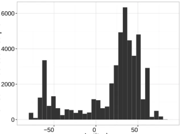
Number of fluorescence profiles

Figure 3.Frequency distribution of the 48 600 profiles of chloro-phyll a concentration and associated phytoplankton community composition in the database as a function of latitude.

and Lewis, 1995), responsible for a decrease in chlorophyll fluorescence values at high irradiance, is not accounted for by the method. The NPQ uncorrected fluorescence profile shape is indeed used to retrieve the vertical distribution of phytoplankton biomass (see details in Sauzède et al., 2015a). Note that, if density profiles are available together with flu-orescence profiles, NPQ can be corrected using the method of Xing et al. (2012). This method involves substituting the fluorescence values acquired within the mixed layer by the maximum value within this layer.

It has been previously mentioned that FLAVOR is not adapted for the retrieval of chlorophyll a concentration on a fluorescence profile-by-profile basis (Sauzède et al., 2015a). Rather, FLAVOR and, hence, the resulting database, are rel-evant for large-scale investigations, e.g., development of cli-matologies of the vertical distribution of chlorophyll a, from which regional anomalies or temporal trends might be

ev-0 2000 4000

1 2 3 4 5 6 7 8 9 10 11 12

Month

Number of fluorescence profiles

Hemisphere

North South

Figure 4.Temporal distribution of the 48 600 profiles of chloro-phyll a concentration and associated phytoplankton community composition in the database as a function of months with black and gray colors, indicating the hemispheres of data acquisition.

idenced. In fact, the method was validated using a global database and it is not excluded that the retrievals from FLA-VOR might be regionally biased. For instance, Sauzède et al. (2015a) have shown that FLAVOR retrievals for the Southern, Arctic and Indian oceans are slightly less accurate than for the other basins. This is likely because the method is not constrained enough in these specific areas which are known for data scarcity. Additional details about the perfor-mance of the method for various oceanic basins are given in Sauzède et al. (2015a), in Figs. S3, S5–S7. Finally, it is worth recalling here that the relationships between the phy-toplankton biomass or community composition profiles and the fluorescence profiles are assumed to be identical for pro-files acquired before 1991 (not involved in the training data set because of lack of HPLC data) and after 1991 (only used for the training process). In the context of possible use of this database for supporting analysis in looking for trends or a shift in chlorophyll a time series, this assumption will have to be taken into consideration.

An additional step of quality control is further applied once the FLAVOR method has been operated. It is based on Chauvenet’s criterion which is used to identify statistical out-liers in the retrieved biomass data (Buitenhuis et al., 2013; Glover et al., 2011; O’Brien et al., 2013). The criterion was applied to the surface data of each profile (median of values from the surface down to 20 m). As Chauvenet’s criterion is based on the assumption that the data follow a normal dis-tribution, the analysis was performed on the log-normalized [TChl] surface values. Such a criterion removes aberrant data partially caused by the failure of the FLAVOR method (see number of profiles removed by Chauvenet’s criterion in Ta-ble 3).

a)

b)

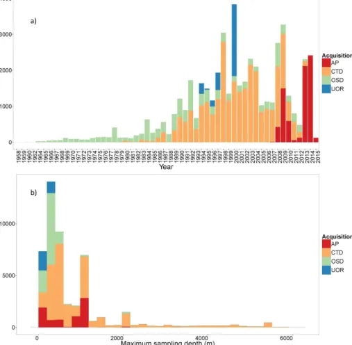
Figure 5.Frequency distribution of the 48 600 profiles of chlorophyll a concentration and associated phytoplankton community composition in the database as a function of: (a) years of acquisition and (b) the maximum depth of acquisition. Colors refer to the different modes of data acquisition.

3 Results and discussion

3.1 Spatial and temporal coverage of the database

The 48 600 chlorophyll fluorescence profiles which success-fully passed all the steps of quality control were transformed into total chlorophyll a concentration and associated phy-toplankton community size indices (i.e., microphytoplank-ton, nanophytoplankton and picophytoplankton) using FLA-VOR (see details in Sect. 2.3). The resulting database cov-ers all ocean basins with more profiles in the Northern Hemisphere (75 %) than in the Southern Hemisphere (25 %, see Figs. 2 and 3). However, the Southern Hemisphere re-mains relatively well represented with the profiles acquired by autonomous platforms and especially by elephant seals equipped with a fluorometer. Few data were acquired in the Indian Ocean and in the tropical South Atlantic and South Pacific (see Fig. 2). The highest numbers of fluorescence profiles are found at the BATS (the Bermuda Atlantic Time-series Study) and HOT (the Hawaii Ocean Time-Time-series) time-series stations, which are located at 31.67◦N–64.17◦W and 22.75◦N–158.00◦W, respectively, and where data

acquisi-tion started in 1988. On the annual scale, the data acqui-sition appears evenly distributed, with a slight underrepre-sentation of autumn months (April to June) in the Southern Hemisphere (Fig. 4). The temporal distribution of fluores-cence profiles in the database covers 56 years from 1958 to the present (Fig. 5a) and most of the observations were collected after the late 1980s. There are fewer observations from 2010 to 2012 because all data generally acquired by ship-based platforms have not been archived yet in the online databases. A significant increase in data density observed be-tween 2013 and 2015 (in 2015, 124 profiles were acquired in half a month) mainly results from data acquired by Bio-Argo profiling floats. Around one-sixth of this global database has been sampled in only 2 years by the Bio-Argo platforms. This illustrates the potential of this new type of acquisition which is expected to dramatically increase the number of collected fluorescence profiles in the future.

Vertically, the database includes values of total chloro-phyll a concentration and associated phytoplankton commu-nity composition from the surface down to a mean sampling

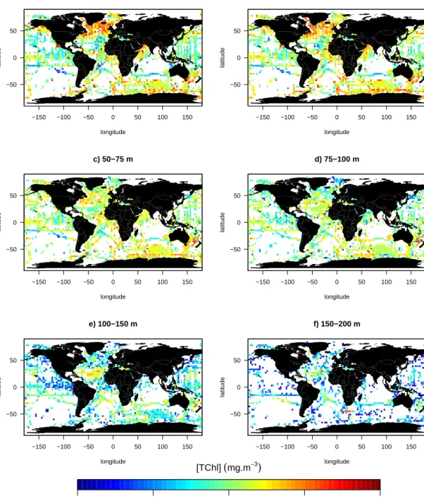
−150 −100 −50 0 50 100 150 −50 0 50 a) 0−25 m longitude latitude −150 −100 −50 0 50 100 150 −50 0 50 b) 25−50 m longitude latitude −150 −100 −50 0 50 100 150 −50 0 50 c) 50−75 m longitude latitude −150 −100 −50 0 50 100 150 −50 0 50 d) 75−100 m longitude latitude −150 −100 −50 0 50 100 150 −50 0 50 e) 100−150 m longitude latitude −150 −100 −50 0 50 100 150 −50 0 50 f) 150−200 m longitude latitude 0.001 0.01 0.1 1 10 [TChl]

(

)

Figure 6.Median total chlorophyll a concentration (mg m−3) scaled to a 3◦spatial resolution for six vertical layers: (a) 0–25 m, (b) 25–50 m,

(c) 50–75 m, (d) 75–100 m, (e) 100–150 m and (f) 150–200 m.

depth of 743 m (with a maximum sampling depth ranging from 100 to 6000 m; Fig. 5b).

3.2 Vertical distribution of the chlorophyll biomass

We present the database with respect to the vertical distribu-tion of the total chlorophyll a concentradistribu-tion ([TChl]). Fig-ure 6 displays the median [TChl] gridded within squares of 3◦latitude by 3◦longitude and over six vertical layers (0–25, 25–50, 50–75, 75–100, 100–150 and 150–200 m). In the

sur-face layer (0–25 m, see Fig. 6a), the [TChl] median is the highest in the North Atlantic and the lowest in the South Pacific subtropical gyre. The median [TChl] decreases with depth for all the data, except for data acquired in South Pa-cific and Atlantic subtropical gyres where the median [TChl] increases with depth. This increase is associated with the so-called deep chlorophyll maximum (DCM) that is typical of these oligotrophic regions (e.g., Cullen, 1982; Mignot et al., 2011, 2014).

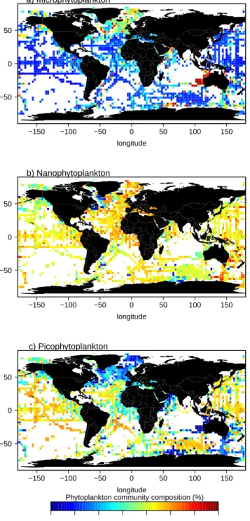
−150 −100 −50 0 50 100 150 −50 0 50 longitude latitude a) Microphytoplankton −150 −100 −50 0 50 100 150 −50 0 50 longitude latitude b) Nanophytoplankton −150 −100 −50 0 50 100 150 −50 0 50 longitude latitude c) Picophytoplankton 0 10 20 30 40 50 60 70

Phytoplankton community composition (%)

Figure 7. Mean relative contribution to the total chlorophyll a biomass (%) for the three phytoplankton size-based groups gridded and scaled to a 3◦resolution within the 0–1.5 Zelayer: (a)

micro-phytoplankton, (b) nanophytoplankton and (c) picophytoplankton.

The global distribution of the phytoplankton community composition, given in terms of fraction of chlorophyll a con-centration associated to micro-, nano- and picophytoplank-ton, is presented for the 0–1.5 Ze layer (Fig. 7a, b and c respectively). Here Ze, the euphotic depth is defined as the depth at which the irradiance is reduced to 1 % of its surface value. It was estimated according to the method of Morel and

Berthon (1989), using the [TChl] profiles derived from FLA-VOR. Figure 7 reveals general geographic patterns which are consistent with the knowledge about the ecological domains and biogeochemical provinces (Longhurst, 2010). On aver-age microphytoplankton are dominant in the subarctic zone, with a relative contribution to the chlorophyll biomass reach-ing more than 70 % in these areas (Fig. 7a). Picophytoplank-ton are dominant in the subtropical gyres (South and North Pacific as well as South and North Atlantic), with a contri-bution reaching 45–55 % (Fig. 7c). Nanophytoplankton ap-pear to be ubiquitous with a relatively stable contribution to biomass of 40–50 % (Fig. 7b).

To further assess the quality, range and representation of the FLAVOR-retrieved [TChl] database presented in this study, the retrieved surface [TChl] is compared to the re-motely sensed [TChl]. In this context, the climatological [TChl] mean was extracted at a 9 km spatial resolution from NASA Modis Aqua archive for the time period cov-ering 2002 to 2014. The extracted satellite [TChl] data were re-gridded to a 3◦×3◦spatial resolution. Similarly the FLAVOR-retrieved [TChl] values for the upper layer of the database (i.e., mean value calculated between the surface and 20 m) for the same period were re-gridded to 3◦×3◦squares. Figures 8 and 9 show that climatological averaged [TChl] from Modis Aqua and from the present database are gener-ally consistent (Fig. 8a and b). The log-transformed ratio of the Modis Aqua to the database [TChl] estimates reveals a rather good agreement with a median value of −0.16 and a standard deviation of 0.58 (see histogram in Fig. 8c). Figure 9 displays the geographic distribution of the log-transformed ratio between the Modis Aqua and the database estimates of climatological surface [TChl]. The ratio shows no specific spatial bias. However, as it is mentioned in Sect. 2.3, FLA-VOR retrievals for the Southern, Arctic and Indian oceans are slightly less accurate than for the other basins; it is there-fore possible that the estimation errors are greater in these areas. Moreover, this observation has to be nuanced consid-ering the difficulties in retrieving accurate ocean color satel-lite [TChl] in these high-latitude environments (Gregg and Casey, 2004; Guinet et al., 2013; Johnson et al., 2013; Pelo-quin et al., 2013; Siegel et al., 2005; Szeto et al., 2011).

3.3 Example of application: climatological time series of the vertical distribution of chlorophylla

concentration and phytoplankton community composition

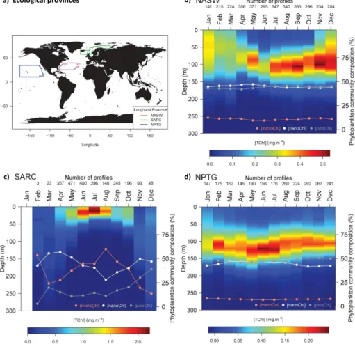
As an example of application, monthly climatologies were computed for three ecological provinces defined by Longhurst (2010) and well represented in the current data set (Fig. 10a): (1) the North Atlantic Subtropical Gyral Province West (NASW, Fig. 10b), (2) the Atlantic Subarctic Province (SARC, Fig. 10c) and (3) the North Pacific Sub-tropical Gyre Province (NPTG, Fig. 10d). Overall the time series of the vertical distribution in [TChl] are consistent

Figure 8.(a) Climatological mean (2002–2014) chlorophyll a

con-centration (mg m−3) from Modis Aqua (scaled to a 3◦resolution);

(b) climatological mean (1958–2015) surface chlorophyll a

concen-tration (mg m−3) from the present database (averaged over the up-per 20 m and scaled to a 3◦resolution); (c) histogram of the log10 ratio of the chlorophyll a concentration from the database to the chlorophyll a concentration from Modis Aqua. The mean, median and standard deviation of the ratio are indicated in the figure. The color scale applies to panels (a) and (b).

−150 −100 −50 0 50 100 150 −50 0 50 longitude latitude log10([TChl]DB[TChl]sat) −2 −1 0 1 2

Figure 9.Geographic distribution of the log10-transformed ratio of the climatological mean surface [TChl] of the database over the upper 20 m of the water column ([TChl]DB) and the climatological

mean satellite [TChl] from Modis Aqua ([TChl]sat). Both [TChl]

data were scaled to a 3◦resolution.

with expectations as detailed by Longhurst (2010). For the NASW province (Fig. 10b), [TChl] is relatively homoge-neous from the surface to around 140 m from January to March; then the stratification of the water column leads to the establishment of a deep chlorophyll maximum (DCM) from April to November. Over the year, [TChl] varies in a restricted range of values (0.35–0.55 mg m−3_{). The} dom-inant phytoplankton groups are the nano- and the picophyto-plankton with relative chlorophyll contribution reaching 40– 45 % for both size-based groups. The contribution of micro-phytoplankton remains low throughout the year (10 %). For the SARC province, the phytoplankton bloom starts in May (as indicated by a significant increase in [TChl], Fig. 10c). The bloom continues for 4 to 5 months with [TChl] within the 1.5–2 mg m−3 range (with maximum values in July). The microphytoplankton contribution increases during the bloom and reaches a maximum (60 %) in August, whereas the nanophytoplankton relative contribution decreases from April to August. The contribution of picophytoplankton in-creases slightly all along the year to reach a maximum of about 40 % in December. For the NPTG province (Fig. 10d), a DCM (0.15–0.25 mg m−3_{) is established at a depth of 100–} 125 m and persists all year long. This DCM deepens in summer, consistently with a deeper light penetration in the water column at this period. The [TChl] at DCM reaches a maximum value in June and July. The dominant phyto-plankton groups are the nano- and the picophytophyto-plankton with relative contribution reaching 45–50 % for both size-based groups and slight opposite temporal evolutions. The

a) Ecological provinces b)

c) d)

Figure 10.Monthly climatologies of the vertical distribution of the total chlorophyll a concentration and associated phytoplankton size-based groups for three ecological provinces defined by Longhurst (2010). (a) Geographic distribution of the considered provinces: North Atlantic Subtropical Gyral Province West (NASW), Atlantic Subarctic Province (SARC) and North Pacific Subtropical Gyre Province (NPTG). Climatologies obtained for the (b) NASW, (c) SARC and (d) NPTG. The color scale indicates the total chlorophyll a concentration (mg m−3); the data points superimposed onto the colored monthly vertical profiles show the percentages of integrated chlorophyll a concentration associated with the micro-, nano- and picophytoplankton within the water column.

contribution of microphytoplankton remains low throughout the year (< 10 %).

4 Conclusions and recommendations for use

The phytoplankton biomass (i.e., chlorophyll a concentra-tion) and phytoplankton community size indices were de-rived from chlorophyll fluorescence profiles using a dedi-cated calibration method (FLAVOR, Sauzède et al., 2015a). For the first time, in situ chlorophyll fluorescence profiles from various data centers have been collected and synthe-sized in a global data set to create unified and interoperable products related to chlorophyll a concentration and phyto-plankton communities. This work can thus be considered as a first step towards the development of a 3-D climatologi-cal representation of chlorophyll a concentration and phy-toplankton community composition. As mentioned before, we recall here that this database should not be used on a profile-by-profile basis. Instead, this database has rather to be

used to derive climatologies from which regional or tempo-ral trends might possibly be extracted. To date, and because of the lack of in situ vertical data, the identification of such trends has been based exclusively on surface remotely sensed data (Beaulieu et al., 2013; Boyce et al., 2010; Gregg, 2005; Gregg et al., 2002). Obviously, the present data set offers a potential refinement to improve open-ocean climatologies of chlorophyll a with respect to the vertical dimension.

Finally, this database has to be considered as a reference that has the potential to evolve. It is now clear that numerous fluorescence profiles will be acquired through robotic obser-vations (e.g., Claustre et al., 2010b; Johnson et al., 2009). In fact, about one-sixth of the profiles of the present database have been sampled by Bio-Argo profiling floats in only 2 years. Therefore the database proposed here represents a first step towards a global single-reference database reconciling the oldest data sets of chlorophyll fluorescence with the fu-ture ones, mostly acquired remotely by autonomous plat-forms.

Acknowledgements. This paper is a contribution to the Remotely Sensed Biogeochemical Cycles in the Ocean (remO-cean) project, funded by the European Research Council (grant agreement 246777), to the French Bio-Argo project funded by CNES-TOSCA and to the French “Equipement d’avenir” NAOS project (ANR J11R107-F). The French PROOF and CYBER programs are acknowledged for their support of cruises where in situ chlorophyll fluorescence profiles were acquired. We are grateful to all the project PIs who contributed data, as well as to the anonymous staff who took part in the data acquisition during the cruises.

Edited by: F. Schmitt

References

Beaulieu, C., Henson, S. A., Sarmiento, Jorge L., Dunne, J. P., Doney, S. C., Rykaczewski, R. R., and Bopp, L.: Factors chal-lenging our ability to detect long-term trends in ocean chloro-phyll, Biogeosciences, 10, 2711–2724, doi:10.5194/bg-10-2711-2013, 2013.

Boyce, D. G., Lewis, M. R., and Worm, B.: Global phyto-plankton decline over the past century, Nature, 466, 591–596, doi:10.1038/nature09268, 2010.

Boyer, T. P., Antonov, J. I., Baranova, O. K., Garcia, H. E., Johnson, D. R., Locarnini, R. A., Mishonov, A. V, O’Brien, T. D., Seidov, D., Smolyar, I. V., and Zweng, M. M.: World Ocean Database 2009, edited by: Levitus, S., 2009.

Buitenhuis, E. T., Vogt, M., Moriarty, R., Bednaršek, N., Doney, S. C., Leblanc, K., Le Quéré, C., Luo, Y.-W., O’Brien, C., O’Brien, T., Peloquin, J., Schiebel, R., and Swan, C.: MAREDAT: towards a world atlas of MARine Ecosystem DATa, Earth Syst. Sci. Data, 5, 227–239, doi:10.5194/essd-5-227-2013, 2013.

Claustre, H.: The trophic status of various oceanic provinces as re-vealed by phytoplankton pigment signatures, Limnol. Oceanogr., 39, 1206–1210, 1994.

Claustre, H., Hooker, S. B., Van Heukelem, L., Berthon, J.-F., Bar-low, R., Ras, J., Sessions, H., Targa, C., Thomas, C. S., van der Linde, D., and Marty, J.-C.: An intercomparison of HPLC phyto-plankton pigment methods using in situ samples: application to remote sensing and database activities, Mar. Chem., 85, 41–61, doi:10.1016/j.marchem.2003.09.002, 2004.

Claustre, H., Antoine, D., Boehme, L., Boss, E., D’Ortenzio, F., D’Andon, O. F., Guinet, C., Gruber, N., Handegard, N. O., Hood, M., Johnson, K., Körtzinger, A., Lampitt, R., LeTraon, P. Y., Lequéré, C., Lewis, M., Perry, M. J., Platt, T., Roemmich, D., Testor, P., Sathyendranth, S., Send, U., and Yoder, J.: Guidelines towards an integrated ocean observation system for ecosystems and biogeochemical cycles, in: Proceedings of the OceanObs 09: Sustained Ocean Observations and Information for Society Con-ference (Vol.1), edited by: Hall, J., Harrison, D. E., and Stammer, D., ESA Publ., Venice, Italy, 2010a.

Claustre, H., Bishop, J., Boss, E., Bernard, S., Johnson, K., Lotiker, A., Ulloa, O., Perry, M. J., Uitz, J., Curie, M., Villefranche, D., Lazaret, C., Division, E. S., Berkeley, L., Road, O. C., Observa-tion, E., Africa, S., Fermi, V., De Brest, C., Valley, O., and Jolla, L.: Bio-optical profiling floats as new observational tools for biogeochemical and ecosystem studies: potential synergies with

ocean color remote sensing, in: Proceedings of the OceanObs 09: Sustained Ocean Observations and Information for Society Con-ference (Vol.2), edited by: Hall, J., Harrison, D. E., and Stammer, D., ESA Publ., Venice, Italy, 2010b.

Conkright, M. E., Locarnini, R. A., Garcia, H. E., O’Brien, T. D., Boyer, T. P., Stephens, C., and Antonov, J. I.: World Ocean Atlas 2001: Objective analyses, data statistics, and figures: CD-ROM documentation, US Department of Commerce, National Oceanic and Atmospheric Administration, National Oceanographic Data Center, Ocean Climate Laboratory, 2002.

Cullen, J. J.: The deep chlorophyll maximum: comparing vertical profiles of chlorophyll a, Can. J. Fish. Aquat. Sci., available at: http://agris.fao.org/agris-search/search.do? recordID=US201302185941 (last access: 23 February 2015), 1982.

Cullen, J. J. and Lewis, M. R.: Biological processes and op-tical measurements near the sea surface: Some issues rel-evant to remote sensing, J. Geophys. Res., 100, 13255, doi:10.1029/95JC00454, 1995.

Cunningham, A.: Variability of in-vivo chlorophyll fluorescence and its implication for instrument development in bio-optical oceanography, Sci. Mar., 60, 309–315, 1996.

Falkowski, P., Kiefer, D. A., Division, O. S., and Angeles, L.: Chlorophyll a fluorescence in phytoplankton: relationship to photosynthesis and biomass, J. Plankton Res., 7, 715–731, 1985. Glover, D. M., Jenkins, W. J., and Doney, S. C.: Modeling Methods for Marine Science, Cambridge University Press, Cambridge, 2011.

Gordon, H. R. and McCluney, W. R.: Estimation of the depth of sunlight penetration in the sea for remote sensing, Appl. Optics, 14, 413–416, doi:10.1364/AO.14.000413, 1975.

Gregg, W. W.: Recent trends in global ocean chlorophyll, Geophys. Res. Lett., 32, L03606, doi:10.1029/2004GL021808, 2005. Gregg, W. W. and Casey, N. W.: Global and regional evaluation of

the SeaWiFS chlorophyll data set, Remote Sens. Environ., 93, 463–479, doi:10.1016/j.rse.2003.12.012, 2004.

Gregg, W. W., Conkright, M. E., Atlantic, N., Chlorophyll, B. O., Indian, S., Pacific, S., and Atlantic, S.: Decadal changes in global ocean chlorophyll, Geophys. Res. Lett., 29, 1–4, 2002.

Guinet, C., Xing, X., Walker, E., Monestiez, P., Marchand, S., Pi-card, B., Jaud, T., Authier, M., Cotté, C., Dragon, A. C., Dia-mond, E., Antoine, D., Lovell, P., Blain, S., D’Ortenzio, F., and Claustre, H.: Calibration procedures and first dataset of South-ern Ocean chlorophyll a profiles collected by elephant seals equipped with a newly developed CTD-fluorescence tags, Earth Syst. Sci. Data, 5, 15–29, doi:10.5194/essd-5-15-2013, 2013. Johnson, K., Berelson, W., Boss, E., Chase, Z., Claustre, H.,

Emer-son, S., Gruber, N., Kortzinger, A., Perry, M., and Riser, S.: Ob-serving Biogeochemical Cycles at Global Scales With Profiling Floats and Gliders Prospects for a Global Array, Oceanography, 22, 216–225, 2009.

Johnson, R., Strutton, P. G., Wright, S. W., McMinn, A., and Mein-ers, K. M.: Three improved satellite chlorophyll algorithms for the Southern Ocean, J. Geophys. Res.-Ocean., 118, 3694–3703, doi:10.1002/jgrc.20270, 2013.

Kiefer, D. A.: Chlorophyll a fluorescence in marine centric diatoms: Responses of chloroplasts to light and nutrient stress, Mar. Biol., 23, 39–46, doi:10.1007/BF00394110, 1973.

Le Quere, C., Harrison, S., Prentice, I., Buitenhuis, E., Aumont, O., Bopp, L., Claustre, H., de Cunha, L., Geider, R., Giraud, X., Klaas, C., Kohfield, K., Legendre, L., Manizza, M., Platt, T., Rivkin, R., Sathyendranath, S., Uitz, J., Watson, A., and Wolf-Gladrow, D.: Ecosystem dynamics based on plankton functional types for global ocean biogeochemistry models, Glob. Chang. Biol., available at: https://ueaeprints.uea.ac.uk/27956/ (last ac-cess: 19 March 2014), 2005.

Levitus, S., Antonov, J. I., Baranova, O. K., Boyer, T. P., Coleman, C. L., Garcia, H. E., Grodsky, A. I., Johnson, D. R., Locarnini, R. A., Mishonov, A. V., Reagan, J. R., Sazama, C. L., Seidov, D., Smolyar, I., Yarosh, E. S., and Zweng, M. M.: The World Ocean Database, Data Sci. J., 12, WDS229–WDS234, 2013.

Longhurst, A. R.: Ecological Geography of the Sea, avail-able at: http://books.google.com/books?hl=fr&lr=&id= QdJZezzrCfQC&pgis=1 (last access: 22 January 2015), 2010.

Lorenzen, C. J.: A method for the continuous measurement of in vivo chlorophyll concentration, Deep Sea Res. Oceanogr. Abstr., 13, 223–227, doi:10.1016/0011-7471(66)91102-8, 1966. McClain, C. R.: A decade of satellite ocean color

observations, Ann. Rev. Mar. Sci., 1, 19–42, doi:10.1146/annurev.marine.010908.163650, 2009.

Mignot, A., Claustre, H., D’Ortenzio, F., Xing, X., Poteau, A., and Ras, J.: From the shape of the vertical profile of in vivo fluores-cence to Chlorophyll-a concentration, Biogeosciences, 8, 2391– 2406, doi:10.5194/bg-8-2391-2011, 2011.

Mignot, A., Claustre, H., Uitz, J., Poteau, A., D’Ortenzio, F., and Xing, X.: Understanding the seasonal dynamics of phyto-plankton biomass and the deep chlorophyll maximum in olig-otrophic environments: A Bio-Argo float investigation, Global Biogeochem. Cycles, 28, 856–876, doi:10.1002/2013GB004781, 2014.

Morel, A. and Berthon, J.-F.: Surface Pigments, Algal Biomass Pro-files, and Potential Production of the Euphotic Layer: Relation-ships Reinvestigated in View of Remote-Sensing Applications, Limnol. Oceanogr., 34, 1545–1562, 1989.

O’Brien, C. J., Peloquin, J. A., Vogt, M., Heinle, M., Gruber, N., Ajani, P., Andruleit, H., Arístegui, J., Beaufort, L., Estrada, M., Karentz, D., Kopczynska, E., Lee, R., Poulton, A. J., Pritchard, T., and Widdicombe, C.: Global marine plankton functional type biomass distributions: coccolithophores, Earth Syst. Sci. Data, 5, 259–276, doi:10.5194/essd-5-259-2013, 2013.

Peloquin, J., Swan, C., Gruber, N., Vogt, M., Claustre, H., Ras, J., Uitz, J., Barlow, R., Behrenfeld, M., Bidigare, R., Dierssen, H., Ditullio, G., Fernandez, E., Gallienne, C., Gibb, S., Goericke, R., Harding, L., Head, E., Holligan, P., Hooker, S., Karl, D., Landry, M., Letelier, R., Llewellyn, C. A., Lomas, M., Lucas, M., Man-nino, A., Marty, J.-C., Mitchell, B. G., Muller-Karger, F., Nel-son, N., O’Brien, C., Prezelin, B., Repeta, D., Jr. Smith, W. O., Smythe-Wright, D., Stumpf, R., Subramaniam, A., Suzuki, K., Trees, C., Vernet, M., Wasmund, N., and Wright, S.: The MARE-DAT global database of high performance liquid chromatography marine pigment measurements, Earth Syst. Sci. Data, 5, 109– 123, doi:10.5194/essd-5-109-2013, 2013.

Sauzède, R., Claustre, H., Jamet, C., Uitz, J., Ras, J., Mignot, A., and D’Ortenzio, F.: Retrieving the vertical distribution of chloro-phyll a concentration and phytoplankton community composi-tion from in situ fluorescence profiles: A method based on a neu-ral network with potential for global-scale applications, J. Geo-phys. Res.-Ocean., 120, 451–470, doi:10.1002/2014JC010355, 2015a.

Sauzède, R., Lavigne, H., Claustre, H., Uitz, J., Schmechtig, C., D’Ortenzio, F., Guinet, C., and Pesant, S.: Global compilation of chlorophyll fluorescence profiles from several data bases, and from published and unpublished individual sources, avail-able at: http://doi.pangaea.de/10.1594/PANGAEA.844212, last access: 19 March 2015b.

Sauzède, R., Lavigne, H., Claustre, H., Uitz, J., Schmechtig, C., D’Ortenzio, F., Guinet, C., and Pesant, S.: Global data prod-uct of chlorophyll a concentration and phytoplankton commu-nity composition (microphytoplankton, nanophytoplankton and picophytoplankton) computed from in situ fluorescence profiles, available at: http://doi.pangaea.de/10.1594/PANGAEA.844485, last access: 19 March 2015c.

Siegel, D. A., Maritorena, S., Nelson, N. B., and Behrenfeld, M. J.: Independence and interdependencies among global ocean color properties: Reassessing the bio-optical assumption, J. Geophys. Res., 110, C07011, doi:10.1029/2004JC002527, 2005.

Siegel, D. A., Behrenfeld, M. J., Maritorena, S., McClain, C. R., Antoine, D., Bailey, S. W., Bontempi, P. S., Boss, E. S., Dierssen, H. M., Doney, S. C., Eplee, R. E., Evans, R. H., Feldman, G. C., Fields, E., Franz, B. A., Kuring, N. A., Mengelt, C., Nelson, N. B., Patt, F. S., Robinson, W. D., Sarmiento, J. L., Swan, C. M., Werdell, P. J., Westberry, T. K., Wilding, J. G., and Yoder, J. A.: Regional to global assessments of phytoplankton dynamics from the SeaWiFS mission, Remote Sens. Environ., 135, 77–91, doi:10.1016/j.rse.2013.03.025, 2013.

Szeto, M., Werdell, P. J., Moore, T. S., and Campbell, J. W.: Are the world’s oceans optically different?, J. Geophys. Res., 116, C00H04, doi:10.1029/2011JC007230, 2011.

Uitz, J., Claustre, H., Morel, A., and Hooker, S. B.: Vertical dis-tribution of phytoplankton communities in open ocean: An as-sessment based on surface chlorophyll, J. Geophys. Res., 111, C08005, doi:10.1029/2005JC003207, 2006.

Vidussi, F., Claustre, H., Manca, B. B., Luchetta, A., and Marty, J.-C.: Phytoplankton pigment distribution in relation to upper ther-mocline circulation in the eastern Mediterranean Sea during win-ter, J. Geophys. Res., 106, 19939, doi:10.1029/1999JC000308, 2001.

Xing, X., Claustre, H., Blain, S., D’Ortenzio, F., Antoine, D., Ras, J., and Guinet, C.: Quenching correction for in vivo chloro-phyll fluorescence acquired by autonomous platforms: a case study with instrumented elephant seals in the Kerguelen region (Southern Ocean), Limnol. Oceanogr. Methods, 10, 483–495, doi:10.4319/lom.2012.10.483, 2012.