HAL Id: insu-02571769
https://hal-insu.archives-ouvertes.fr/insu-02571769
Submitted on 13 May 2020
HAL is a multi-disciplinary open access
archive for the deposit and dissemination of sci-entific research documents, whether they are pub-lished or not. The documents may come from teaching and research institutions in France or abroad, or from public or private research centers.
L’archive ouverte pluridisciplinaire HAL, est destinée au dépôt et à la diffusion de documents scientifiques de niveau recherche, publiés ou non, émanant des établissements d’enseignement et de recherche français ou étrangers, des laboratoires publics ou privés.
Radar? Results from an experiment in the Äspö
Hardrock Laboratory, Sweden
Justine Molron, Niklas Linde, Ludovic Baron, Jan-Olof Selroos, Caroline
Darcel, Philippe Davy
To cite this version:
Justine Molron, Niklas Linde, Ludovic Baron, Jan-Olof Selroos, Caroline Darcel, et al.. Which
fractures are imaged with Ground Penetrating Radar? Results from an experiment in the
Äspö Hardrock Laboratory, Sweden. Engineering Geology, Elsevier, 2020, 273, pp.105674.
Which fractures are imaged with Ground Penetrating Radar?
Results from an experiment in the Äspö Hardrock Laboratory,
Sweden
Justine Molron, Niklas Linde, Ludovic Baron, Jan-Olof Selroos,
Caroline Darcel, Philippe Davy
PII:
S0013-7952(19)32273-2
DOI:
https://doi.org/10.1016/j.enggeo.2020.105674
Reference:
ENGEO 105674
To appear in:
Engineering Geology
Received date:
4 December 2019
Revised date:
5 May 2020
Accepted date:
7 May 2020
Please cite this article as: J. Molron, N. Linde, L. Baron, et al., Which fractures are
imaged with Ground Penetrating Radar? Results from an experiment in the Äspö Hardrock
Laboratory,
Sweden,
Engineering
Geology
(2020),
https://doi.org/10.1016/
j.enggeo.2020.105674
This is a PDF file of an article that has undergone enhancements after acceptance, such
as the addition of a cover page and metadata, and formatting for readability, but it is
not yet the definitive version of record. This version will undergo additional copyediting,
typesetting and review before it is published in its final form, but we are providing this
version to give early visibility of the article. Please note that, during the production
process, errors may be discovered which could affect the content, and all legal disclaimers
that apply to the journal pertain.
Which fractures are imaged with Ground Penetrating Radar? Results from an
experiment in the Äspö Hardrock Laboratory, Sweden
Justine MOLRON1,*, Niklas LINDE2, Ludovic BARON2, Jan-Olof SELROOS3, Caroline DARCEL1 and
Philippe DAVY4
1
Itasca Consultants S.A.S., 64 Chemin des Mouilles, 69130 Ecully, France
j.molron@itasca.fr* & c.darcel@itasca.fr
2
Institut des sciences de la Terre, Université de Lausanne, Géopolis UNIL, Quartier Mouline, 1015 Lausanne, Switzerland.
niklas.linde@unil.ch & ludovic.baron@unil.ch
3
Swedish Nuclear Fuel and Waste Management Company (SKB), Evenemangsgatan 13, Box 3091, SE-169 03 Solna, Sweden.
jan-olof.selroos@skb.se
4
Géosciences Rennes, OSUR, CNRS, Université de Rennes 1, 263 Avenue Général Leclerc, 35042 Rennes, France.
philippe.davy@univ-rennes1.fr
Abstract
Identifying fractures in the subsurface is crucial for many geomechanical and hydrogeological
applications. Here, we assess the ability of the Ground Penetrating Radar (GPR) method to image
open fractures with sub-mm apertures in the context of future deep disposal of radioactive waste.
GPR experiments were conducted in a tunnel located 410 m below sea level within the Äspö Hard
Rock Laboratory (Sweden) using 3-D surface-based acquisitions (3.4 m x 19 m) with 160 MHz, 450
MHz and 750 MHz antennas. The nature of 17 identified GPR reflections was analyzed by means of
three new boreholes (BHBH3; 9-9.5 m deep). Out of 21 injection and outflow tests in packed-off
1-m sections, only five provided responses above the detection threshold with the 1-maxi1-mu1-m
transmissivity reaching 7.0 × 10⁻¹⁰ m2/s. Most GPR reflections are situated in these permeable regions
and their characteristics agree well with core and Optical Televiewer data. A 3-D statistical fracture
model deduced from fracture traces on neighboring tunnel walls show that the GPR data mainly
identify fractures with dips between 0 and 25°. Since the GPR data are mostly sensitive to open
fractures, we deduce that the surface GPR method can identify 80% of open sub-horizontal fractures.
We also find that the scaling of GPR fractures in the range of 1-10 m2 agrees well with the statistical
model distribution indicating that fracture lengths are preserved by the GPR imaging (no
measurement bias). Our results suggests that surface-GPR carries the resolution needed to identify
the most permeable sub-horizontal fractures even in very low-permeability formations, thereby,
suggesting that surface-GPR could play an important role in geotechnical workflows, for instance, for
industrial-scale siting of waste canisters below tunnel floors in nuclear waste repositories .
Key words: Ground Penetrating Radar, surface-based method, fracture, core log, tunnel, statistical
fracture model, nuclear waste disposal
1. Introduction
In hard rock systems, fractures are the main conduit for flow (Becker & Shapiro, 2000), for
contaminant transport (Selroos et al., 2002), and they play a critical role in determining the
mechanical properties of rocks (Davy et al., 2018a). Hydrogeological and geomechanical applications
require, henceforth, an appropriate characterization of the fracture network and of its hydrological
and mechanical properties (Davy et al., 2018a). Traditionally, this information is mostly derived from
a statistical analysis of 2-D fracture traces mapped in tunnel walls and surface outcrops, or from 1-D
fracture intercepts along boreholes. Such statistical approaches have drawbacks: 1) the 3-D fracture
models do not rely on actual 3-D observations, which requires crude assumptions on some fracture
properties (e.g., fracture shapes) (Davy et al., 2018b); 2) some scales are hardly measured because of
the limited size of outcrops, tunnel walls, or borehole diameter; 3) models that aim at making
predictions are generally better constrained by conditioning to location-specific deterministic
information than by global statistics only (Andersson & Dverstorp, 1987). This is why imaging
fractures at different scales, especially with non-invasive methods, is of high importance for
hydrogeological and geomechanical applications (e.g. mine and tunnel stability, detection of flow
paths, contaminant transport).
A particular application, which partly motivates this study, is the detection of potential pathways (at
the 10 m scale) from defective canisters for nuclear waste with non-invasive (i.e., without drilling)
surface methods. This is required to identify locations that are unsuitable for storing nuclear waste in
canisters emplaced under the tunnel floor, as envisioned for the storage of nuclear waste in Finland
and Sweden. In the very low-permeability formations that are of interest for the nuclear waste
repositories of Sweden or Finland, transport of potentially released radionuclides take place through
fractures with sub-millimetric apertures that are very difficult to detect remotely. This excludes
many geophysical methods such as seismic reflection/refraction, electrical resistivity and nuclear
magnetic resonance for this task. If one adds both the constraint of being surface-based and being
able to detect meter-scale individual fractures remotely, the only suitable method is ground
penetrating radar (GPR) (Day-Lewis et al., 2017).
There is a rich literature describing how GPR data were used to detect permeable fractures in various
hydrogeological (Becker & Tsoflias, 2010; Day-Lewis et al., 2003; Dorn et al., 2011a; Dorn et al.,
2011b; Dorn et al., 2012; Shakas et al., 2016; Tsoflias et al., 2001), geotechnical (Davis & Annan,
1989; Grasmueck et al., 2005; Grégoire & Halleux, 2002; Seol et al., 2001) and nuclear waste-related
(Baek et al., 2017; Döse & Carlsten, 2017; Olsson et al., 1992; Serzu et al., 2004) applications.
Notably, the GPR reflections caused by fracture planes are enhanced when the fractures are
fluid-filled or have large apertures (Grasmueck, 1996; Hollender & Tillard, 1998; Hollender et al., 1999;
Jeannin et al., 2006; Markovaara-Koivisto et al., 2014; Shakas & Linde, 2017; Tsoflias & Becker, 2008;
Tsoflias & Hoch, 2006). Electromagnetic (EM) waves with wavelengths on the m-scale respond to
fractures with sub-millimetric aperture because of the strong contrast in electrical properties
between the fracture filling and the surrounding rock matrix and because of multiple internal
reflections between the fracture walls generating wavelet interferences (the thin-bed response)
(Bradford & Deeds, 2006; Deparis & Garambois, 2008; Grégoire & Hollender, 2004; Sassen & Everett,
2009; Shakas & Linde, 2015). At repository depth (~400-600 m below sea level), the fracture aperture
can be very small and it is not yet clear whether observed GPR reflections in such an environment are
primarily related to water-filled fractures and not to other geological interfaces (e.g., dike intrusion,
geological contacts, material-filled fractures). It is also not clear which percentage of open fractures
are imaged as a function of their sizes and orientations.
In this contribution, we present a 3-D GPR imaging experiment performed at 410 m depth in the
Äspö Hard Rock Laboratory, Sweden (Figure 1a). The GPR data have been migrated to form a 3-D
network of reflectors, hereafter, named GPR fractures. After the GPR experiment, three 9-m deep
boreholes were drilled in the zone (Figure 1b), mapped with televiewer logging, and hydraulically
tested to ground-truth the GPR results.
Our main aims are to address the following questions:
1. Do GPR reflections observed in deep low-permeability granitic formations correspond to
open transmissive fractures only or also to other types of geological discontinuities?
2. What is the detection accuracy of the GPR fractures in terms of fracture sizes and
orientations?
The first point has been addressed by a careful GPR experiment performed in a 410-m deep tunnel
by picking the main reflectors and verifying the nature of reflectors from a subsequent drilling of
three boreholes analyzed by core logging and hydraulic tests. The second point has been addressed
by comparing the statistics of GPR fractures with the 3-D fracture statistics derived from outcrop and
borehole mapping.
2. Test Site
The Äspö Hard Rock Laboratory (HRL) is an underground research facility below the island of Äspö
located approximately 300 km south of Stockholm on the peninsula of Simpevarp surrounded by the
Baltic Sea (Figure 1a). It was constructed in 1986 (Cosma et al., 2001) by the Swedish Nuclear Fuel
and Waste Management Company (SKB) as a R&D site to develop new methodologies and
technologies to build the know-how needed to construct a hard rock repository for nuclear waste. It
contains a main tunnel of 3.6 km length and several side-tunnels extending from the surface down to
450 m depth (Figure 1a) (SKB, 2016). The geology is mainly composed of fractured granitic rocks that
are more than 1.7 billion years old (Cosma et al., 2001).
The GPR investigation focuses on the secondary TAS04 tunnel, which was excavated at a depth of
410 m by the drill-and-blast method (Ericsson et al., 2015; Ericsson et al., 2018). The tunnel is 36 m
long, 4.2 m wide and 5.3 m high. Its geology is composed by three main rock types: fine-grained
granite, Äspö diorite and Ävrö granodiorite, with some pegmatite veins (Figure 1b) (Ericsson et al.,
2015; Ericsson et al., 2018). Geotechnical (check of drilling and charging), geological (fracture
mapping), geophysical (surface GPR) and hydrogeological (42 borehole drillings of 2 m depth and
hydraulic tests) investigations were used to characterize superficial fractures induced by the blasting.
It was found that the excavation-damage zone (EDZ) was 0.5 m thick (Ericsson et al., 2015; Ericsson
et al., 2018). The EDZ was removed by cutting and sawing the tunnel floor with a diamond wire along
20 m of the tunnel length; it is in the resulting very flat area that our GPR measurements were
performed (Figure 1b).
In addition to the TAS04 tunnel, three surrounding tunnels at the same depth are used to de rive the
3-D statistical fracture model. The TAS05 and TASN tunnels are parallel to the TAS04 and are 17 m
and 52 m long, 4.5 m and 4.2 m wide and 4.5 m and 3.7 m high, respectively. The TASP tunnel is
perpendicular to the others and is 57 m long, 7 m wide and 4.1 m high.
Figure 1: (a) Illustration of the Äspö Hard Rock Laboratory in the Simpevarp peninsula, Sweden. The study tunnel (TAS04) is situated at a depth of 410 m. Figure modified from SKB (2016), courtesy of SKB, Illustrator: Jan Rojmar. (b) Orthophotography of the tunnel floor showing the geological limit between fine -grained granite (to the left), Äspö diorite and Ävrö granodiorite (to the right) indicated by yellow and blue dashed lines, shallow pre -existing boreholes represented by black dots with oxidation (orange traces) and concrete plates delimited by red dashed lines. The three new boreholes (BH1, BH2 and BH3 indicated by red circles with crosses) were drilled in the granitic formation with locations chosen based on the GPR results. (Figure size: 2 column fitting; Colors: yes)
3. GPR experiment methodology
3.1. GPR survey
The GPR data from the TAS04 tunnel were acquired in the period of November 6-10, 2017, using the
MALÅ GroundExplorer (GX) HDR-serie (High Dynamic Range), equipped with skid plate and wheel.
160, 450 and 750 MHz antennas were used to achieve different investigation depths and image
resolutions. The acquisition parameters are given in Table 1. The shielded transmitter and receiver
antennas, separated by a fixed separation in a so-called common-offset configuration (Annan, 2003),
were pulled along the cleaned and flat tunnel floor (Figure 2). The GPR profiles were acquired with
2.34 cm measurement spacing and a line separation of 0.05 m for the 450 and 750 MHz surveys and
0.10 m for the 160 MHz survey. The profiles were oriented along the tunnel length (x-direction) using
multiple orthogonal measurement tapes to ensure straight and parallel measurement lines. The
resulting acquisition area was 3.4 m × 19 m. Measurements with a total station using fixed geodetic
points in the tunnel were used to convert the acquisition geometry into the local Äspö coordinate
system (Äspö96).
Table 1: Experimental parameters used for the 3-D GPR acquisitions in common-offset mode. (Table size: 2 column fitting)
Parameters Frequencies (MHz) 160 450 750 Antenna separation (m) 0.33 0.18 0.14 Measurement spacing (m) 0.02355 0.02355 0.02355 Profile separation (m) 0.10 0.05 0.05 Number of profiles 34 69 69 Investigation depth (m) 0 to 10 0 to 8 0 to 5
Journal Pre-proof
Figure 2: (a) The common-offset GPR configuration: the transmitter (Tx) and receiver (Rx) antennas are placed in a shielded box. The surface GPR is pulled along the tunnel floor (x-direction). The transmitter antenna sends an electromagnetic pulse into the subsurface and the receiver antenna records the returning signal amplitudes over time as shown schematically in (b). (Figure size: 2 column fitting; Colors: yes)
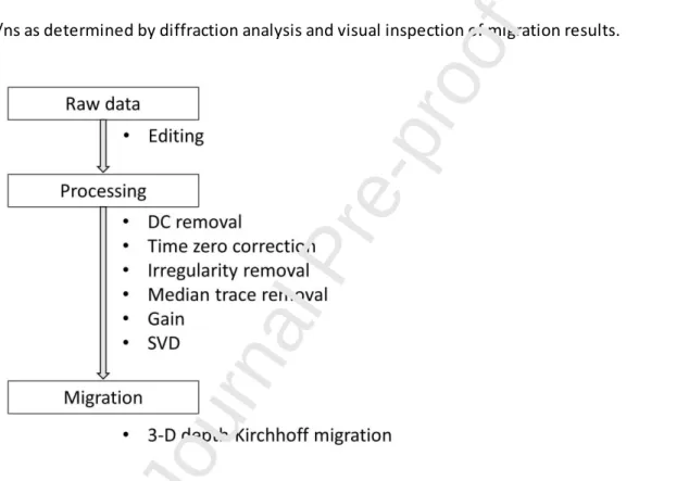
3.2. Data processing
The GPR data processing and migration workflow is depicted in Figure 3. We consciously avoid
automatic gain control to enable relative comparisons of reflectivity at different locations in the
investigated volume. The editing step involves removal of some limited data at the end of certain
profiles to ensure a rectangular-shaped survey area. Direct Current (DC) removal used to remove
offsets in the data is achieved by subtracting the mean of the last 33% of the GPR traces. Time zero
corrections are made to ensure that the actual source initiation time is treated as zero. For each
trace, this is achieved by shifting the time vector such that the time when the signal magnitude is
first above the noise-level corresponds to the time it takes for the speed of light in a vacuum to travel
the distance between the source and receiver. Irregularity removal refers to traces that are adversely
affected by the many (42) shallow boreholes (0-1 m depth) and two concrete plates. To avoid the
migration of these data that largely respond to non-geologic features, we automatically detected
(5-6% of the data) and removed these traces by identifying irregularities in the magnitudes of their
direct waves. Median trace removal along each line was performed to not only remove the direct
wave, but also significant ringing in the data. Time-gain with a different exponent for each frequency
(2.5 for 160 MHz, 2.5 for 450 MHz and 2.0 for 750 MHz data) was applied to correct for geometric
spreading and attenuation of later-arriving signals. Finally, singular value decomposition (SVD) was
used to remove the first 3 to 5 singular values to further suppress ringing effects.
Migration was needed to collapse the many diffractors in the data and to properly locate the
reflections at depth. For this, we used 3-D depth Kirchhoff migration (Margrave & Lamoureux, 2019)
as implemented in the CREWES Matlab toolbox (CREWES, 1988) with a constant velocity of 0.130
m/ns as determined by diffraction analysis and visual inspection of migration results.
Figure 3: Flow chart describing how the raw data are edited and processed before migration. (Figure size: 1 column fitting;
4. Results
The 3-D GPR results are exemplified by processed profiles of 160 MHz (Figure 4), 450 MHz (Figure 5)
and 750 MHz (Figure 6) data and corresponding 3-D migration results along a 2-D section located
approximately in the middle of the tunnel. As expected, the 750 MHz data have the highest
resolution and the lowest investigation depth, while the 160 MHz data have the lowest resolution
and the highest investigation depth. The 450 MHz is the most suitable frequency for identifying each
individual feature from 0 to 8 m depth. To a first order, the vertical and horizontal resolution
enabling separation of features in migrated images are , where is the wavelength (Annan, 2003;
Grasmueck, 2005; Jol, 2008; Reynolds, 1997). Since the average wave speed is 0.13 m/ns, the vertical
and horizontal resolutions are 0.2 m for 160 MHz, 0.06 m for 450 MHz and 0.04 m for 750 MHz.
The unmigrated data (Figure 4a, Figure 5a, Figure 6a) show diffractions manifested by characteristic
hyperbolas. The shallow diffractions are mainly caused by the shallow boreholes (42), while deeper
diffractions may be related to fracture wall irregularities, fracture intersections or geological
heterogeneities (Grasmueck et al., 2015; Grasmueck et al., 2013; Grasmueck et al., 2005). On depth
slices, these diffractions appear as concentric circles, whose radii are increasing with depth (Figure
7a).
To remove the diffractions and locate the reflections in space, we used 3-D Kirchhoff migration with
a constant velocity of 0.13 m/ns. After migration, the energy contained in the hyperbola tails is
ideally gathered into a unique point corresponding to the initial diffraction point ( Figure 7b). After
migration, sub-horizontal reflections that might correspond to fractures are visible on vertical 2-D
GPR slices with alternating positive and negative amplitudes aligned in sub-horizontal patterns
(Figure 4b, Figure 5b, Figure 6b). This alternation is a consequence of the finite-length source wavelet
used by the GPR antennas. Sub-vertical features that might correspond to fractures appear as bright
spots plunging with depth that are clearly visible in the horizontal GPR depth slices (Figure 7b, c).
To visualize the GPR results in three dimensions, we imported 2-D processed and migrated data slices
into the software Paradigm GOCADTM (Figure 8) using Äspö coordinates. By comparing unmigrated
(Figure 4a, Figure 5a, Figure 6a) and migrated (Figure 4b, Figure 5b, Figure 6b) data for the three
frequencies, we created a simplified fracture network model (Figure 8). This manual procedure of
identifying GPR fractures is somewhat subjective. Large sub-horizontal GPR structures were picked
on each vertical 2-D slice at the interface between the background signal and the signal
corresponding to the reflection of the structure represented by positive (intense white) or negative
(intense black) amplitudes. Sub-vertical fractures were identified on horizontal depth slices by picking
their horizontal edge traces (Figure 7c). The set of the trace picks was used to construct the fracture
surface using the convex hull plane that connects the picks, with no assumption on fracture form in
order to avoid over- or underestimation of the data. We identified a total of 21 reflections that might
correspond to fractures with dimensions of 1 to 4 m. This work was focused on the first 15 m of the
GPR block along the axis of the tunnel, in order to be within the same fine-grained granitic
environment (Figure 8).
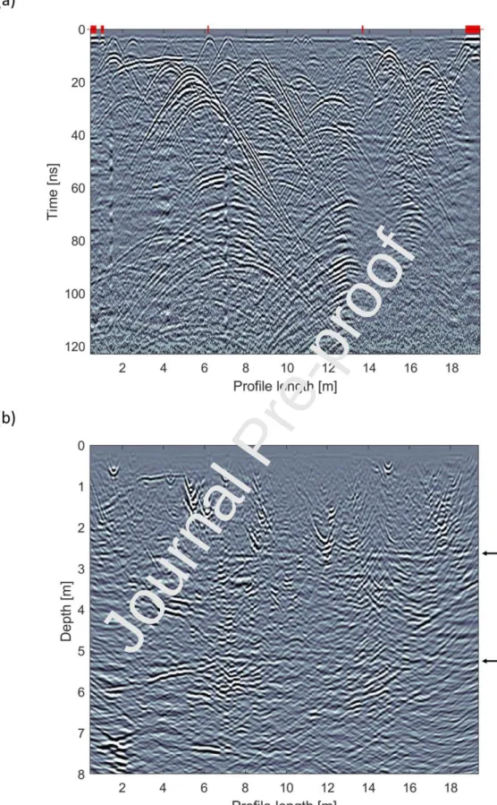
Figure 4: (a) Processed 2-D GPR slice acquired with 160 MHz antennas at y = 2.25 m. Red plus signs correspond to shallow boreholes and concrete plate irregularities; the corresponding traces are removed before migration. (b) Migrated data based on 3-D Kirchhoff migration with a constant velocity of 0.13 m/ns. The time and depth inte rvals are chosen based on the associated resolution and depth of penetration. (Figure size: 2 column fitting; Colors: yes)
Figure 5: (a) Processed 2-D GPR slice acquired with 450 MHz antennas at y = 2.28 m. Red plus signs correspond to shallow boreholes and concrete plate irregularities; the corresponding traces are removed before migration. (b) Migrated data based on 3-D Kirchhoff migration with a constant velocity of 0.13 m/ns. The depth interval is chosen based on the associated resolution and depth of penetration. The large horizontal features at depths of 2.5 and 5.1 m (indicated by black horizontal arrows) are attributed to reflections at the tunnel roof and corresponding multiples. (Figure size: 2 column fitting; Colors:
Figure 6: (a) Processed 2-D GPR slice acquired with 750 MHz antenna at y = 2.28 m. Red plus signs correspond to shallow boreholes and concrete plate irregularities; the corresponding traces are removed before migration. (b) Migrated data based on 3-D Kirchhoff migration with a constant velocity of 0.13 m/ns. The depth interval is chosen based on the associated resolution and depth of penetration. The large horizontal feature at a depth of 2.5 m (indicated by a black horizontal arrow) is attributed to reflections at the tunnel roof. (Figure size: 2 column fitting; Colors: yes)
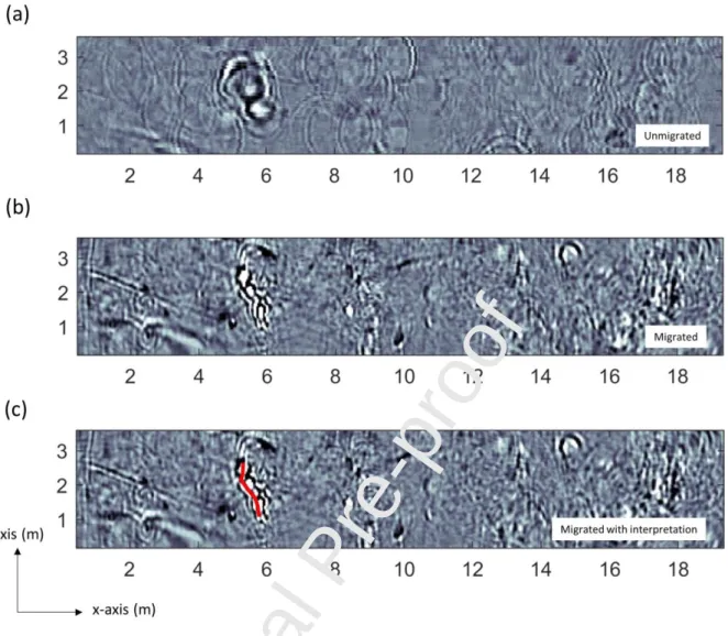
Figure 7: Depth slices obtained from 450 MHz data at 1.32 m depth illustrating diffractions that are likely due to sub-vertical fractures. (a) Unmigrated processed data for which the diffractions are represented by circular shapes. (b) Migrated data in which the diffractions collapse and (c) the corresponding sub-vertical features can be identified manually. (Figure size: 2 column fitting; Colors: yes)
5. Verification of GPR fractures with borehole data
Based on our simplified GPR fracture model, we sited three boreholes of 9.0 to 9.5 m depth with a
diameter of 0.076 m: BH1 (K04018G02) in a region with multiple sub-horizontal reflections that we
expected would correspond to an overall more transmissive region, BH2 (K04022G02) in a region of
prominent sub-vertical reflections and diffractions with an expected significant transmissivity and
BH3 (K04026G02) in a region with few GPR reflections suggesting that it would contain fewer open
fractures and be less permeable than BH1 and BH2 (Figure 8). Because of technical constraints, the
boreholes had to be separated by at least 3 m and located at a certain distance away from the 42
shallow pre-existing boreholes and concrete plates. The final locations of the boreholes are seen in
Figure 1b.
After drilling, BH1 was sealed and its pressure was monitored during the drilling of BH2 and BH3. The
same procedure was followed for BH2 during the drilling of BH3. This provides useful information
about the hydraulic connections between boreholes. All boreholes were cored and imaged with a
televiewer in order to map intersecting fractures. The orientation and openness of the intersecting
fractures were subsequently determined from these data.
Figure 8: Fence diagrams displaying the migrated 450 MHz data. (a) The migrated GPR data based on which three boreholes (BH1, BH2 and BH3) were drilled. The basis for the borehole design is illustrated in (b) where GPR reflections corresponding to expected fractures are displayed. The strong reflections were manually picked at the interface between the background signal and the signal corresponding to the reflection of the structure. The fracture planes were constructed by the convex hull method and the fractures intersecting the boreholes are represented in red. Reflections are only interpreted in the region of fine-grained granite (first 15 m). (Figure size: 2 column fitting; Colors: yes)
5.1. Connectivity between boreholes
During the drilling of BH2, the pressure in BH1 showed two periods of net decreases (Figure 9a)
corresponding to the boring of sections from 3.2 to 3.5 m depth and from 7.1 to 7.5 m depth. This
suggests that BH1 is at least connected to fractures at these two section depths in BH2. During the
drilling of BH3, pressure in BH1 (not shown) and BH2 (Figure 9b) showed similar behavior with three
distinct decreases corresponding to the boring of BH3 in the sections from 1.9 to 2.9 m, 4.9 to 5.2 m
and 6.4 to 6.9 m depth, respectively. Due to the vicinity to BH3, the pressure drop in BH2 is three
times higher than in BH1. Finally, the stationary pressure (1850 kPa in BH1, 2050 kPa in BH2 and 2150
kPa in BH3) in each packed-off borehole indicates a strong hydraulic gradient from BH3 towards BH1.
Figure 9: Pressure responses observed in observation boreholes while drilling new boreholes. Pressure response in (a) BH1 during the drilling of BH2 and (b) BH2 during the drilling of BH3. The first part of the curves (yellow) represents pressure rise due to the installation of a mechanical packer in drilled borehole at 1 m depth. The initiations of pressure drops (blue, green and orange) correspond to drilling of borehole sections (3.2-3.5 m and 7.1-7.5 m in BH2 and 1.9-2.2, 4.9-5.2 m and 6.4 m in BH3). A subsequent smaller pressure decrease is also observed in BH2 (blue part) corresponding to the drilling between 2.7 and 2.9 m in BH3. (Figure size: 2 column fitting; Colors: yes)
5.2. Hydraulic tests
The hydraulic properties of the fractured rock were estimated from injection and outflow tests in
1-m packed-off sections fro1-m 1 to 8 1-m depth (Andersson &a1-mp; Ragvald, 2019) by 1-means of a High pressure
Water Injection Controller (HWIC) equipment (Hjerne et al., 2013) that automatically measures the
injection or outflow with a constant imposed pressure. Most of the tests (Table 2) were performed
with outflowing conditions due to the very high ambient borehole pressure (approximately 2000
kPa). In some sections, the pressure could not return to its initial state quickly enough after an
outflow test and injection tests were performed.
Of the 21 1-m sections being tested, only 5 sections (3 for BH1, 1 for BH2 and 1 for BH3) provided a
flow rate above the measuring limit of the flowmeter (2 mL/min). Hydraulic transmissivities of the
1-m sections were then esti1-mated by Andersson and Ragvald (2019) using Moye’s for1-mula (Moye,
1967) assuming that steady-state was reached at the end of each test:
, (1)
, (2)
where is the hydraulic transmissivity (m2/s); is the flow rate at the end of the flow duration
(m3/s); is the water density (kg/m3); is the acceleration of gravity (m/s2); is the geometrical
shape factor; is the injection/outflow pressure differences; is the measurement section
length and is the borehole radius (m). Based on the results (Table 2), the rock is found to have a
very low transmissivity with the five 1-m sections above the detection limit having transmissivities
ranging between 2.2-7.0 × 10⁻¹⁰ m2/s.
The boreholes with the transmissive zones highlighted are plotted together with crossing migrated
450 MHz GPR slices in Figure 10. Strong and large sub-horizontal reflections traversing the boreholes
are highlighted. Four such reflections are identified near BH1 with three of them being situated in the
transmissive zone. Along BH2, six strong (but not very large) reflectors are identified with two being
situated in the transmissive zone. No strong reflectors are identified along BH3.
Table 2: Results of hydraulic tests in 1-m packed-off sections for each borehole (BH1 to BH3) using High pressure Water Injection Controller (HWIC) equipment (Hjerne et al., 2013). Pressure measured in each 1-m test section shows the variation due to the hydraulic disturbance: injection tests give positive pressures and outflow tests give negative pressures. Hydra ulic transmissivity was calculated from Moye’s formula (Moye, 1967). (2 column fitting)
Borehole ID Test section
(m) Pressure (kPa) Flow rate (L/min) Hydraulic transmissivity (m2/s) BH1 1-2 200 < detection limit 2-3 510 < detection limit 3-4 -1427 -0.0033 2.2E-10 4-5 -1086 -0.0073 6.3E-10 5-6 -1080 -0.0065 5.6E-10 6-7 -1449 < detection limit 7-8 -1376 < detection limit BH2 1-2 656 < detection limit 2-3 -1875 < detection limit 3-4 -1589 -0.0038 2.2E-10 4-5 400 < detection limit 5-6 -1979 < detection limit 6-7 -1600 < detection limit 7-8 -1979 < detection limit BH3 1-2 175 < detection limit 2-3 -833 < detection limit 3-4 191 < detection limit 4-5 -1300 -0.0097 7.0E-10 5-6 -1600 < detection limit 6-7 -1659 < detection limit 7-8 -1300 < detection limit
Journal Pre-proof
Figure 10: Fence diagrams displaying migrated data (450 MHz) crossing each borehole (BH1, BH2 and BH3). The yellow vertical line segments indicate transmissive 1-m sections as determined by water injection tests, while the red sections induce less flow than the detection limit of 2 mL/min. Transmissive 1-m sections are located between 3 and 6 meters depth in BH1, between 3 and 4 m of depth in BH2 and between 4 and 5 m depth in BH3. Uninterpreted GPR sections along BH1 (a), BH2 (b) and BH3 (c) and interpreted GPR sections where strong reflections are represented in full blue lines, while blue dashed lines correspond to the potential extensions of the reflectors along BH1 (d), BH2 (e) and BH3 (f). (Figure size: 2 column fitting; Colors: yes)
5.3. Fracture mapping
Fracture characteristics (e.g., position, depth, strike, dip, filling mineralogy, open/sealed information)
were obtained by Optical Televiewer (OPTV) and core logging (Andersson & Ragvald, 2019). With the
position and orientation information, we could implement the fractures into our database, describing
the fractures as disks centered on the boreholes. This enables a detailed assessment of the
agreement between the GPR reflections and the fractures seen in the core logging (Figure 11, Figure
12, Figure 13).
We present the fracture positions in terms of depth, orientation (strike and dip) and opening (sealed
or open) using tadpole plots (Figure 11a, Figure 12a and Figure 13a). This interpretation is based on
televiewer and core inspection in the laboratory. Each borehole is represented by a cylinder divided
into 1-m sections used for hydraulic measurements with indication of GPR reflections crossing the
borehole and the sections with recorded outflows above the measurements limit (Figure 11b, Figure
12b and Figure 13b). Fence diagrams are used to highlight strong GPR reflections along the boreholes
and to compare them with fractures seen on cores (Figure 11c,d, Figure 12c,d and Figure 13c). To do
so, we superimposed fractures from core log data on the GPR sections crossing the borehole, and
observed the match based on fracture depth, strike and dip. We assume that a GPR fracture matches
a fracture intersection trace if their depth and dip do not exceed a deviation of 0.3 m and 15°,
respectively (Table 3). The strike is also used to assess the fracture matching, but its uncertainty is
particularly high for sub-horizontal fractures. Consequently, we used a maximum strike deviation of
60°. The corresponding fracture intercepts are well seen in the OPTV images (Figure 11e,f, Figure
12e,f and Figure 13d).
Along BH1 (Figure 11), we observed four strong reflections that match very well with four fractures
seen on cores. The maximum disagreement in terms of fracture depth, dip and strike are 0.1 m, 6°
and 54°, respectively (Table 3). The fractures have all been interpreted as open and three of them are
located in the transmissive region (above the flow measurement threshold) while the remaining
fracture is located in the 0 to 1 m interval where no hydraulic tests were made. We note that this
corresponds to a rather ideal case for GPR data, as the identified transmissive fractures all have low
dips for which the GPR reflections are the strongest.
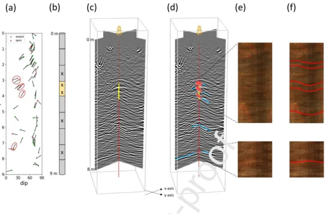
Figure 11: Comparison of core log, hydraulic and GPR data for BH1. (a) Tadpole plot representing the fracture characteristics (depth, orientation and aperture) along the borehole. The circle symbols show the fracture localization in term of depth (y-axis) according to their dip (x-(y-axis). The red and green colors correspond to the open and sealed fractures. The ended black tails represent the direction of the dip, with North (0° and 360°), East (90°), South ( 180°) and West (270°) being up, right, down and left respectively. The fractures matching by the depth, dip and/or strike with GPR reflectors are encircled in red. (b) Borehole representation with transmissive sections (yellow) and strong reflections (cross in the middle of the sections). Fence diagrams display migrated GPR data (450 MHz) crossing BH1 (c) before and (d) after interpretation. The identified transmissive zones are represented in yellow and fractures logged along the borehole and matching (by depth, strike and/or dip) with strong GPR reflections (blue lines) are symbolized by red disks (open fracture) centered on the borehole . (e) Uninterpreted and (f) interpreted Optical Televiewer images showing the fracture traces on borehole walls. Fractures matching with GPR reflectors are underlined in red lines. Yellow depth scale corresponds to the depth recorded by the Televiewer. (Figure size: 2 column fitting; Colors: yes)
Along BH2 (Figure 12), five reflections have been identified (Figure 10) that are generally less strong
than those crossing BH1. Since the fractures observed in this borehole are mostly composed by
sub-vertical fractures (75%), the surface GPR data contain multiple diffractions (Figure 5) that clutter the
resulting migrated images and make the match with any sub-horizontal fractures non-trivial. This
superposition of energy is particularly present in the area situated between 2.8 and 3.8 m. The two
first reflections seem to match with two sets of closely separated sub-horizontal fractures that are
interpreted as open. Each set is composed by two fractures separated by 0.1 m. The first set is well
correlated in terms of depth, dip and strike with the first reflector. The second set is well correlated
in terms of depth and strike with the second reflector while the dip is above the threshold. The third
reflection matches well in terms of depth, dip and strike with a fracture at 3.7 m of depth (Table 3).
These five open fractures are concentrated in the zone where flow could be measured (the first
fracture is situated at 0.1 m above this measured section). The strong reflector that appears to cross
the borehole at 5.7 m depth does not correspond to any borehole fractures. Such a mismatch can be
explained by the fact that borehole data give punctual information while GPR gives a measure that is
averaged on a roughly metric scale. This implies that the geological heterogeneity or fracture
corresponding to this reflection could be next to the borehole. The last reflector, matching in terms
of depth, strike and dip with an open fracture at 7.4 m, is located in the borehole section (7.13 to
7.54 m) that produced a pressure response in BH1 during the drilling of BH2. Even if its transmissivity
could not be determined because of the flowmeter threshold, it does provide a strong GPR
reflection. This suggests that this fracture is locally less permeable at the borehole location, which is
also indicated by the GPR reflectivity that is significantly increased away from the borehole.
Figure 12: Comparison of core log, hydraulic and GPR data for BH2. (a) Tadpole representing the fracture characteristics (depth, orientation and aperture) along the borehole. The circle symbols show the fracture localization in term of depth (y-axis) according to their dip (x-(y-axis). The red and green colors correspond to the open and sealed fractures. The ended black tails represent the direction of the dip, with North (0° and 360°), East (90°), South (180°) and West (270°) being up, right, down and left respectively. The fractures matching by the depth, dip and/or strike with GPR reflectors are encircled in red. (b) Borehole representation with transmissive sections (yellow) and strong reflections (cross in the middle of the sections) Fence diagrams display migrated GPR data (450 MHz) crossing BH2 (c) before and (d) after interpretation. The ide ntified transmissive zones are represented in yellow and fractures logged along the borehole and matching (by depth, strike and/or dip) with strong GPR reflections (blue lines) are symbolized by red disks (open fracture) centered on the borehole . (e) Uninterpreted and (f) interpreted Optical Televiewer images showing the fracture traces on borehole walls. Fractures matching with GPR reflectors are underlined in red lines. Yellow depth scale corresponds to the depth recorded by the Televiewer. (Figure size: 2 column fitting; Colors: yes)
BH3 is mostly composed by sub-vertical (90%) and sealed (80%) fractures that highly limit the
possibility of imaging fractures with the surface GPR method. In the transmissive region, all open
fractures have dips exceeding 60°. Consequently, no GPR fracture was identified (Figure 10, 13).
The match between GPR data and borehole data (pressure, hydraulic and core logging data), for BH1
and BH2, shows that fractures interpreted by GPR are mostly situated in the mo st transmissive
hydraulic sections measured along boreholes. Most remaining GPR reflections showed correlation
with depth sections being connected to other boreholes (pressure measurements) or matched with
fractures from borehole (core log data). In one case, it had to be assumed that the fracture was
positioned just next to the borehole. The reason that no fracture is seen by GPR along BH3, despite
that it contains the most permeable 1-m section, is explained by the significant number of
sub-vertical fractures, highlighting the well-known fact that surface-based GPR is unable to image very
steeply dipping fractures.
Figure 13: Comparison of core log, hydraulic and GPR data for BH3. (a) Tadpole plot representing the fracture characteristics (depth, orientation and aperture) along the borehole. The circle symbols show the fracture localization in term of depth (y-axis) according to their dip (x-(y-axis). The red and green colors correspond to the open and sealed fractures. The ended black tails represent the direction of the dip, with North (0° and 360°), East (90°), South (180°) and West (270°) being up, right, down and left respectively. (b) Borehole representation with transmissive sections (yellow). No strong GPR reflections are listed. Fence diagrams display migrated GPR data (450 MHz) crossing BH3 (c). The identified transmissive zone is represented in yellow. No reflector is seen along the BH3 and no matching could be done. (d) Optical Televiewer images showing the transmissive zone composed mostly by open fractures with dips >60°. Yellow depth scale corresponds to the depth recorded by the Televiewer. (Figure size: 2 column fitting; Colors: yes)
Table 3: Matching criteria based on the depth, strike and dip comparison between GPR reflectors (R) and core logged fractures (F). A maximum threshold was defined: 0.3 m for depth, 15° for dip and 60° for strike. The matching criteria is validated when the gap (calculated by subtracting values from R and F) is below the threshold (v). Any values above this threshold are rejected (x). (2 column fitting)
Boreh ole ID
Depth (m) Strike (° N) Dip (°) Matching criteria
R F Gap R F Gap R F Gap Depth Strike Dip
BH1 0.7 0.7 0 166 141 25 10 16 6 v v v 3.7 3.7 0 123 69 54 22 22 0 v v v 4.2 4.1 0.1 141 104 37 24 30 6 v v v 5.6 5.5 0.1 188 218 30 8 11 3 v v v BH2 2.9 2.9 0 181 161 20 27 29 2 v v v 3.0 0.1 149 32 33 6 v v v 3.2 3.2 0 117 128 11 6 42 36 v v x 3.3 0.1 125 8 37 31 v v x 3.7 3.7 0 84 119 35 30 44 14 v v v 5.7 / / 102 / / 18 / / x x x 7.4 7.4 0 329 298 30 11 18 7 v v v
6.
Statistical completeness and GPR agreement
The proportion of existing fractures that are identified by GPR likely depends on the fracture size,
orientation and filling content. In order to estimate this ratio, we derived the 3-D orientation and size
distribution of fractures from the fracture traces observed in the surrounding tunnel walls. The
following sections describe the methodology used and compare the density of GPR-observed
fractures to the expected values derived from this 3-D density distribution.
6.1. Tunnel data (size and orientation distributions of fracture traces)
In addition to the tunnel (TAS04) in which the GPR experiment was carried out, we also used
information from two parallel (TAS05 and TASN) and one perpendicular tunnel (TASP). A total of
3513 fracture traces have been observed on tunnel walls and stored in the SKB database together
with their fracture characteristics: trace length, orientation (dip and strike), aperture, mineral filling
and fracture shape. The trace length density distribution per unit surface is shown in Figure 14. It
exhibits two different scaling behaviors above and below 3.6 m even after removing censoring and
edge biases (Laslett, 1982), that is, fracture traces smaller than 1 m and larger than 8.6 m. The
observed trend is fitted by a power law with a scaling exponent of -2 for small traces and -3 for large
ones. This two-power-law trace size distribution model is consistent with the analysis of outcrop
maps in the same area (Davy et al., 2010).
The stereonet of fracture trace orientation poles (i.e., one pole per fracture) is given in Figure 15a. It
shows three main orientation poles: two vertical ones trending NW and NE, and one horizontal. The
comparison of the fracture trace orientation with those of the GPR fractures is described in section
6.3.
Figure 14: Trace and fracture length density distribution per unit surface and volume, respectively. The trace length distribution is represented by black dots corresponding to the number of fracture traces observed on tunnel walls normalized by tunnel surfaces (y-axis), in size ranges using logarithmic binning. The fits of the trend are represented by light and dark gray curves for fractures smaller and larger than 3.6 m, following a power law. The corresponding 3-D distribution (black curve) was calculated from stereological rules (Piggott, 1997) applied to trace data. (Figure size: 2 column fitting; Colors: no)
Figure 15: Stereonet representation (equal area projection) showing fracture orientation poles (black dots). The strike is indicated around the circle, with North (0° and 360°), East (90°), South (180°) and West (270°) being up, right, down and lef t respectively while the dip is seen from the middle (0°) to the edge of the stereonet (90°). The densi ty color scale represents the fracture density distribution according to orientation units, explaining higher density values for GPR fracture orientations. Tunnel orientations are represented by dark (TASP) and light (TAS04, TAS05 and TASN) gray triangles. (a) Representation of the fracture trace orientation poles (3513) showing two vertical trending (NW and NE) following the tunnel directions and one horizontal (middle of stereonet), (b) fracture pole orientations imaged by GPR (17) showing a horizontal trend of the fractures. (Figure size: 2 column fitting; Colors: yes)
6.2. 3-D statistical model
The 3-D statistical model is calculated by assuming disk-shaped fractures and that the orientation
distribution is similar for all fracture sizes in the target range (1-8 m). The statistical model is based
on trace size distribution and orientation developed in section 6.1 and its consistency has been
checked on three realizations.
The 3-D distribution parameters (density and power law exponent terms) are calculated according to
the stereological rules described by Piggott (1997). These rules were initially applied for an infinite
surface with fractures having uniform orientation. Nevertheless, they have been tested by several
simulations for non-uniform fractures sampled on cylindrical tunnels and it shows that Piggott’s rules
can be applied for fractures sampled on tunnel walls (Appendix A). For a power law and assuming
that fractures are disk shaped, the relation is:
(3)
√
( )
( ) (4)
and are the 2-D and 3-D exponents of fracture traces and sizes, respectively, and
and are the density terms in 2-D and 3-D, respectively. The calculated 3-D density parameters
are and for fracture sizes between 1 m and 4.2 m and and
for fracture lengths above 4.2 m.
The fracture orientations are calculated from the occurrence of fracture traces by applying a
weighting factor equal to the angular correction of Mauldon and Mauldon (1997) for a cylindric
tunnel and fracture sizes smaller than the tunnel diameter:
√ (5)
where is the angle between the fracture pole and the tunnel direction.
We verify from direct simulations (i.e., calculating fracture traces from a 3-D fracture network
generated with the size and orientation distribution deduced from equations (3), (4) and (5)) that the
model is consistent with data, and consequently that:
The cylindric-shape assumption is valid even if tunnels have more complex shapes;
The two-power-law model is required to honor the observed trace distribution. We check that the large-scale power-law regime is distinct from the finite-size effect due to the tunnel
diameter.
Considering the density and orientation characteristics, the 3-D distribution of fracture sizes is then
calculated (Figure 14), which gives the number of fractures per unit area, per unit pole angle and per
unit volume.
6.3. Comparison with GPR fracture distribution
The comparison with the orientation distribution deduced from fracture traces shows that the GPR
fracture orientation (picked from all frequencies) corresponds to the sub-horizontal poles (dip <35°)
of the fracture traces (Figure 15b). Since the GPR has imaged the fractures with area from 1 to 10m2
and dip less than 35°, we compared the same fracture population in the 3-D statistical model. We
first estimated the detection capacity of GPR by dividing the observed density ( total surface by unit
of volume per dip range) with the 3-D modeled density calculated in the section 6.2 (Figure 16a). The
observed fluctuations between 0 and 20-25° may be due to the limited number GPR fractures, but
there is a clear cut-off of detection above 25° even if some GPR fractures are detected between
25-35°. On average, 5.5% of the fractures with area of 1-10 m2 were detected by GPR. This result is a
direct consequence of the geometry of the GPR antenna, where the surface-based acquisition favors
the imaging of sub-horizontal fractures. This ratio rises to 42% for any type of fracture apertures
(opened or sealed) when considering fractures dipping less than 25°. The ratio of open fractures in
the borehole data (Table 4) is 53% for fractures dipping less than 25°. Assuming that this is also the
ratio for 1-10 m2 fractures, we find that the GPR method is likely imaging 80% of the open fractures
with dip <25°.
According to the GPR fracture dip cut-off, the area distribution of GPR fractures have been calculated
(e.g., number of fractures per unit area and unit volume) for all fractures dipping less than 25° (Figure
16b). In a log-log plot, it appears to follow the same power-law trend as the 3-D modeled area
distribution. The dashed line represents the plot of the modeled distribution area for fractures in the
same dip range considering that 80% of the actual fractures are detected. A remarkable result is that
it fits well the GPR data within the data uncertainties (Figure 16b). The fact that the fracture area
distribution in the range 1-10 m2 is similar to the 3-D area distribution modeled by extrapolating the
tunnel fracture traces means that the GPR is able to image the fractures in proportion to the length
distribution trend (no size selection). This is a promising result, but it does not offer a definite
conclusion because of the small number of GPR fractures, and because of the uncertainty on the
modeled distribution due to the assumptions used.
Table 4: Ratio of GPR detection according to fracture parameters: dip and aperture. Analysis is focused on the open fractures intersecting the boreholes (BH1 to BH3), dipping less than 25°.
Fracture parameters Borehole fractures GPR
Dip Aperture Number Imaging probability
0-90° open + sealed 188 5.5 % < 25° < 25° open + sealed 19 41.6 % open 10 (52.6 %) 79.1 %
Journal Pre-proof
Figure 16: (a) GPR detection capacity for open and sealed (left y-axis) and open (right y-axis)fractures having an area between 1 and 10 m2 according to the dip (x-axis). The detectability cut-offs are represented by black dashed curves (b) Comparison of the modeled 3-D density and GPR density distribution. The area distribution of GPR fractures (y-axis) included in area ranges using an overlapping logarithmic binning (x-axis). Gray bars represent the data uncertainties corresponding to bin limits. The 3-D density model deduced from fracture traces comprised in dip ranges of 90°], 25°] and [0-25°]*80% are represented by black curve, green curve and dashed green curve, respectively. (Figure size: 2 column fitting; Colors: yes)
7. Conclusions and perspectives
The purpose of this work was to assess the ability of the GPR method to image fractures with
sub-millimetric aperture in a very low permeable crystalline rock. To do so, we performed surface -based
measurements in a tunnel situated at 410 m depth. GPR profiles were measured in a 3-D
configuration (3.4 m x 19 m) using three frequencies (160, 450 and 750 MHz). A total of 17
sub-horizontal reflections were manually picked from the 3-D acquisition block, whose minimum and
maximum length were 0.8 m and 5 m, respectively. To define the nature of these reflections, three
boreholes (BH1-BH3; 9-9.5 m deep) were drilled. A very good correlation in terms of depth and
orientation between the GPR reflections crossing BH1 and BH2 and the open transmissive fractures
dipping < 35° located in boreholes was established. The lack of reflections along BH3 is explained by
the sub-vertical orientation of the fractures crossing the borehole.
We derived a 3-D statistical fracture density model from fracture traces observed on surrounding
tunnels walls. This density model predicts the expected number of fractures in the domain for given
orientations and sizes, thereby, enabling comparison with the distribution of GPR fractures. The
comparison is made for fracture areas in the range 1-10 m2, which contains most of the GPR
fractures detected by 160, 450 and 750 MHz antennas. The percentage of fractures detected by GPR
is:
- 5.5 % of all the observed fractures regardless of orientation or if they are open or sealed;
- 42 % of the fractures dipping less than 25°;
- 80 % of open fractures dipping less than 25°.
In addition, the dependency with size of the GPR fracture density distribution is similar to the real
fracture density distribution. Both size distributions fit perfectly if one considers the sub-network of
open fractures dipping less than 25°. This result indicates that there is no size selection in the range
of 1-10 m2 by GPR imaging (the ratio between the fracture size is conserved).
We conclude that GPR imaging can be very efficient to detect open horizontal fractures with
sub-millimeter aperture. The resolution of the present statistical analysis is limited to ~1 m, mainly
because of the cut-off of fracture traces during the tunnel mapping, which constrained the
comparative analysis to this minimum fracture size. The largest fractures and the fracture
orientations are limited by the geometry of the acquisition setup. Further work is planned to use
time-lapse GPR imaging for tracing solute transport in the fracture network similarly to Dorn et al.
(2011b) and Shakas et al. (2016). The main objective of this experiment is to hydraulically
characterize the fracture media and identify the potential conduit for flows.
Appendix A: Piggott stereology tested on non-uniform orientation and
cylindrical outcrops
Piggott (1997) derived the stereological rules that give the 3-D size distribution of uniformly-oriented
disk fractures from a power-law size distribution of fracture traces measured on an infinite plane :
√
( ) ( )
with and being the 2-D and 3-D exponents of fracture traces and sizes, respectively, and
and being the density terms in 2-D and 3-D, respectively.
Here we test whether similar rules can be applied to a finite cylindrical tunnel. For this, we run 3-D
simulations where fracture networks are generated with a power-law size distribution and
non-uniform orientations, and fracture traces are identified on the wall of a cylindric tunnel. We then
calculate the trace size distributions, fit them with a power law, and compare the fit with Piggott’s
formulae (Figure A 1). The ratio between the power-law fits and Piggott’s formulae reaches 1.5, 1.2,
1.1 and 1 for of 2.0 (1652131 fractures and 2834 fracture traces), 2.5 (1156665 fractures and
1479 fractures traces), 3.0 (924152 fractures and 1007 fracture traces) and 3.5 (786477 fractures and
791 traces) respectively. To support our analysis, we compare the fracture trace size distribution
observed on tunnel walls with our statistical model generated with a double power-law size
distribution and orientation bootstrapped from data (Figure A 2).
Figure A 1: Trace length density distributions (lines with circles) deduced from 3D simulations ran according to a single power-law and different exponents ( terms). Solid lines are the expected fits calculated by stereological rules and dashed
lines are the real fits. (Figure size: 2 column fitting; Colors: yes)
Figure A 2: Comparison of fracture trace density distribution between the data (yellow) and the statistical model (green) using Piggott’s stereological rules. The red and blue curves are the fits for fractures smaller and larger than 3.6 m , respectively. (Figure size: 2 column fitting; Colors: yes)
Acknowledgements
This research is part of the ENIGMA ITN project that has received funding from the European Union's
Horizon 2020 research and innovation programme under the Marie Sklodowska-Curie Grant
Agreement No 722028. We thank SKB for its great support, particularly Lars Andersson, Patrik
Vidstrand and Siren Bortelid Robertsson. The GPR data and core log data are stored in the Sicada
database and can be made available after an official request to SKB. We also thank Geosigma,
particularly Peter Andersson and Johanna Ragvald, for their quality fieldwork and detailed report and
Christian Le Carlier De Veslud from Géosciences Rennes for his valuable help to use Paradigm
GOCADTM. Two constructive reviews from anonymous reviewers are greatly appreciated. Finally, this
research is also supported by the French National Observatory H+. The GPR data in WGS84
coordinates are available (after requesting login ID and password through
http://hplus.ore.fr/en/database/acces-database) at
http://hplus.ore.fr/en/molron-et-al-2020-eg-data.
BIBLIOGRAPHY
Andersson, J., & Dverstorp, B. (1987). Conditional simulations of fluid flow in three‐ dimensional networks of discrete fractures. Water Resour. Res., 23(10), 1876-1886.
doi:https://doi.org/10.1029/WR023i010p01876
Andersson, P., & Ragvald, J. (2019). ENIGMA - Poject. GPR monitoring of fractures at Äspö HRL,
Results of field investigations in TAS04 at Äspö HRL, (P-19-17). Retrieved from Stockholm,
Sweden
Annan, P. (2003). Ground penetrating radar principles, procedures and applications. Retrieved from Mississauga, ON, Canada
Baek, S. H., Kim, S. S., Kwon, J. S., & Um, E. S. (2017). Ground penetrating radar for fracture mapping in underground hazardous waste disposal sites: A case study from an underground research tunnel, South Korea. J. Appl. Geophys., 141, 24-33. doi:
https://doi.org/10.1016/j.jappgeo.2017.03.017
Becker, M., & Tsoflias, G. (2010). Comparing flux‐ averaged and resident concentration in a fractured bedrock using ground penetrating radar. Water Resour. Res., 46(9). doi:
https://doi.org/10.1029/2009WR008260
Becker, M. W., & Shapiro, A. M. (2000). Tracer transport in fractured crystalline rock: Evidence of nondiffusive breakthrough tailing. Water Resour. Res., 36(7), 1677-1686.
Bradford, J. H., & Deeds, J. C. (2006). Ground-penetrating radar theory and application of thin-bed offset-dependent reflectivity. Geophysics, 71(3), K47-K57. doi:
https://doi.org/10.1190/1.2194524
Cosma, C., Olsson, O., Keskinen, J., & Heikkinen, P. (2001). Seismic characterization of fracturing at the Äspö Hard Rock Laboratory, Sweden, from the kilometer scale to the meter scale. Int. J.
Rock Mech. Min., 38(6), 859-865. doi: https://doi.org/10.1016/S1365-1609(01)00051-X
CREWES. (1988). CREWES Matlab Toolbox. https://www.crewes.org/ResearchLinks/FreeSoftware/. (accessed 20 November 2017)
Davis, J. L., & Annan, A. P. (1989). Ground-Penetrating Radar for High-resolution mapping of soil and rock stratigraphy. Geophys. Prospect., 37(5), 531-551. doi: https://doi.org/10.1111/j.1365-2478.1989.tb02221.x
Davy, P., Darcel, C., Le Goc, R., & Mas Ivars, D. (2018a). Elastic properties of fractured rock masses with frictional properties and power law fracture size distributions. J. Geophys. Res.: Solid
Earth, 123(8), 6521-6539. doi:https://doi.org/10.1029/2017JB015329
Davy, P., Darcel, C., Le Goc, R., Munier, R., Selroos, J.-O., & Mas Ivars, D. (2018b). DFN, why, how
and what for, concepts, theories and issues. Paper presented at the 2nd International Discrete
Fracture Network Engineering Conference.
Davy, P., Le Goc, R., Darcel, C., Bour, O., De Dreuzy, J. R., & Munier, R. (2010). A likely universal model of fracture scaling and its consequence for crustal hydromechanics. J. Geophys. Res.:
Solid Earth, 115(B10411). doi: https://doi.org/10.1029/2009JB007043
Day-Lewis, F. D., Lane, J. W., Harris, J. M., & Gorelick, S. M. (2003). Time-lapse imaging of saline-tracer transport in fractured rock using difference-attenuation radar tomography. Water
Resour. Res., 39(10). doi: https://doi.org/10.1029/2002wr001722
Day-Lewis, F. D., Slater, L. D., Robinson, J., Johnson, C. D., Terry, N., & Werkema, D. (2017). An overview of geophysical technologies appropriate for characterization and monitoring at fractured-rock sites. J. Environ. Manage., 204, 709-720.
Deparis, J., & Garambois, S. (2008). On the use of dispersive APVO GPR curves for thin-bed
properties estimation: Theory and application to fracture characterization. Geophysics, 74(1), J1-J12. doi: https://doi.org/10.1190/1.3008545
Dorn, C., Linde, N., Doetsch, J., Le Borgne, T., & Bour, O. (2011a). Fracture imaging within a granitic rock aquifer using multiple-offset single-hole and cross-hole GPR reflection data. J.
Appl. Geophys., 78, 123-132. doi: https://doi.org/10.1016/j.jappgeo.2011.01.010
Dorn, C., Linde, N., Le Borgne, T., Bour, O., & Baron, L. (2011b). Single-hole GPR reflection imaging of solute transport in a granitic aquifer. Geophys. Res. Lett., 38(8). doi: https://doi.org/10.1029/2011gl047152
Dorn, C., Linde, N., Le Borgne, T., Bour, O., & Klepikova, M. (2012). Inferring transport
characteristics in a fractured rock aquifer by combining single-hole ground-penetrating radar reflection monitoring and tracer test data. Water Resour. Res., 48(11). doi:
https://doi.org/10.1029/2011wr011739
Döse, C., & Carlsten, S. (2017). Investigation for identification of potential geological signatures for
geophysical objects, (P-11-34). Retrieved from Stockholm, Sweden
Ericsson, L., R, C., Lehtimäki, T., Ittner, H., Hansson, K., Butron, C., Sigurdsson, O., & Kinnbom, P. (2015). A demonstration project on controlling and verifying the excavation-damaged zone, (R-14-30). Retrieved from Stockholm, Sweden
Ericsson, L., Vidstrand, P., Christiansson, R., & Morosini, M. (2018). Comparison Between Blasting
and Wire Sawing Regarding Hydraulic Properties of the Excavated Damaged Zone in a Tunnel–Experiences From Crystalline Rock at the Ӓspӧ Hard Rock Laboratory, Sweden.
Paper presented at the 52nd US Rock Mechanics/Geomechanics Symposium. Grasmueck, M. (1996). 3-D ground-penetrating radar applied to fracture imaging in gneiss.
Geophysics, 61(4), 1050-1064. doi: https://doi.org/10.1190/1.1444026
Grasmueck, M., Moser, T. J., Pelissier, M. A., Pajchel, J., & Pomar, K. (2015). Diffraction signatures of fracture intersections. Interpretation, 3(1), SF55-SF68. doi: http://dx.doi.org/10.1190/INT-2014-0086.1
Grasmueck, M., Quintà, M. C., Pomar, K., & Eberli, G. P. (2013). Diffraction imaging of sub-vertical fractures and karst with full-resolution 3D ground-penetrating radar. Geophys. Prospect.,
61(5), 907-918. doi: https://doi.org/10.1111/1365-2478.12004
Grasmueck, M., Weger, R., & Horstmeyer, H. (2005). Full-resolution 3D GPR imaging. Geophysics,
70(1), K12-K19. doi: https://doi.org/10.1190/1.1852780
Grasmueck, M. W., Ralf ; Horstmeyer, Heinrich (2005). Full-resolution 3D GPR imaging.
Geophysics, 70(1).
Grégoire, C., & Halleux, L. (2002). Characterization of fractures by GPR in a mining environment.
First Break, 20(7), 467-471.
Grégoire, C., & Hollender, F. (2004). Discontinuity characterization by the inversion of the spectral content of ground penetrating radar (GPR) reflections—Application of the Jonscher model.
Geophysics, 69(6), 1414-1424. doi: https://doi.org/10.1190/1.1836816
Hjerne, C., Ludvigsson, J. E., Harrström, J., Olofsson, C., Gokall-Norman, K., & Walger, E. (2013).
Äspö Hard Rock Laboratory. Single-hole injection tests in boreholes KA2051A01, KA3007A01 and KJ0050F01, (P-13-24). Retrieved from Stockholm, Sweden
Hollender, F., & Tillard, S. (1998). Modeling ground-penetrating radar wave propagation and reflection with the Jonscher parameterization. Geophysics, 63(6), 1933-1942. doi: https://doi.org/10.1190/1.1444486
Hollender, F., Tillard, S., & Corin, L. (1999). Multifold borehole radar acquisition and processing.
Geophys. Prospect., 47(6), 1077-1090. doi: https://doi.org/10.1046/j.1365-2478.1999.00166.x
Jeannin, M., Garambois, S., Grégoire, C., & Jongmans, D. (2006). Multiconfiguration GPR
measurements for geometric fracture characterization in limestone cliffs (Alps). Geophysics,
71(3), B85-B92. doi: https://doi.org/10.1190/1.2194526
Jol, H. M. (2008). Ground penetrating radar theory and applications. Amsterdam, The Netherlands: Elsevier.
Laslett, G. M. (1982). Censoring and Edge Effects in Areal and Line Transect Sampling of Rock Joint Traces. Math. Geol., 14(2), 125-140.
Margrave, G. F., & Lamoureux, M. P. (2019). Numerical Methods of Exploration Seismology: With
Algorithms in MATLAB®: Cambridge University Press.
Markovaara-Koivisto, M., Hokkanen, T., & Huuskonen-Snicker, E. (2014). The effect of fracture aperture and filling material on GPR signal. B. Eng. Geol. Environ., 73(3), 815-823. doi: https://doi.org/10.1007/s10064-013-0566-4
Mauldon, M., & Mauldon, J. G. (1997). Fracture sampling on a cylinder: From scanlines to boreholes and tunnels. Rock Mech. Rock Engng., 30(3), 129-144.
Moye, D. G. (1967). Diamond drilling for foundation exploration. Inst Engrs Civil Eng
Trans/Australia/, 9(1), 95-100.