HAL Id: hal-03250815
https://hal.archives-ouvertes.fr/hal-03250815
Preprint submitted on 5 Jun 2021
HAL is a multi-disciplinary open access
archive for the deposit and dissemination of
sci-entific research documents, whether they are
pub-lished or not. The documents may come from
teaching and research institutions in France or
abroad, or from public or private research centers.
L’archive ouverte pluridisciplinaire HAL, est
destinée au dépôt et à la diffusion de documents
scientifiques de niveau recherche, publiés ou non,
émanant des établissements d’enseignement et de
recherche français ou étrangers, des laboratoires
publics ou privés.
A balanced watershed decomposition method
Application to HEC-RAS
Sleimane Hariri, Sylvain Weill, Jens Gustedt, Isabelle Charpentier
To cite this version:
Sleimane Hariri, Sylvain Weill, Jens Gustedt, Isabelle Charpentier. A balanced watershed
decompo-sition method Application to HEC-RAS. 2021. �hal-03250815�
A balanced watershed decomposition method
Application to HEC-RAS
Sleimane Hariria, Sylvain Weillb, Jens Gustedta,c, Isabelle Charpentiera
aICube UMR 7357, Universit´e de Strasbourg and CNRS, 67412 Illkirch, France bLHyGeS UMR 7517, Universit´e de Strasbourg and CNRS, 67000 Strasbourg, France
cINRIA, France
Abstract
Hydrological models are used for water management plans and risk assessment. Based on more and more complex nonlinear partial differential equations, their solution at a watershed level is time and memory consuming for both academic and commercial software. Domain decomposition together with parallelization offer opportunities for faster computations that possibly use larger data sets, as long as a certain balance between the tasks is maintained.
Starting from a digital elevation model and an outlet, we propose a GIS tool for the generation of an area balanced partition of watersheds. For the sake of general usability, the HEC-RAS software together with the HECRASCon-troller tool are chosen for the solution of the hydrological sub-problems. Numerical simulations of a rural watershed assess the sought properties of the domain decomposition and shows the potential gains of the method in terms of parallelization.
Key words: Watershed partitioning, Area balancing, Hydrological models, Partial differential equations, Parallel computing
1. Introduction
Hydrological models widely support the management of water resources, the forecasting of floods, the assess-ment of hazards [1, 2], the simulation of extreme event scenarios [3], and landscape modifications [4].
Since the mid-eighties [5, 6], nonlinear partial dif-ferential equations (PDEs) and additional physical pa-rameterizations allow for the account of more and more complex hydrological processes. Carried out on either a grid or an unstructured mesh, the computational load of their iterative solution is all the more time and memory consuming when the modeled zone is large.
Several parallel computing strategies have been pro-posed to balance the computational load over a multi-processor cluster. In a hydrological context, either the watershed itself or the linear system can be split in order to solve smaller problems.
On the one hand, a sparse parallel solver may be implemented as in the HEC-RAS software [7]. This method is generally more efficient on a multi-core pro-cessor.
On the over hand, GIS tools may be used to split the watershed into a number of hydrological sub-units so
as to split the PDE problem into a number of boundary value sub-problems. A domain decomposition method (DDM) then organizes the solution by gathering the so-lutions computed for the sub-units and by setting rele-vant boundary conditions at the interfaces.
In practice, the watershed partition is usually carried out at the stream confluences [8, 9]. As no guarantee is brought on the balance of the sub-unit areas, the result-ing linear systems are generally of very different sizes and the efficiency of parallelized DDM is limited. As an improvement to that, Pontes et al. [10] use the reach length as a criterion for a decomposition, which reduces the sizes of the largest sub-units, but has not much im-pact on the size of the smallest ones.
In Section 3 of this paper we describe how flow accumulation information may be used to produce an area balanced partition of the watershed and the re-lated load-balanced DDM. For the sake of general us-ability, the HEC-RAS software and HECRASController tool are chosen for the solution of the hydrological sub-problems. Technical solutions are recalled to overcome some issues well-known to practitioners.
The paper is organized as follows. A brief state-of-the-art on the partitioning methods is provided in
tion 2 to highlight requirements and design opportuni-ties. The area balanced partition process and its cou-pling with the HEC-RAS software are presented in Sec-tion 3. DecomposiSec-tion and parallelizaSec-tion results are discussed in Section 4. Finally, Section 5 provides a summary and an outlook.
2. Watershed partition methods
The simulation of large-scale watersheds may involve a large amount of data and long computational times. Consequently, sequential or parallel domain decompo-sition methods are widely used to face memory and time shortages.
In hydrology, a drainage basin may be partitioned into smaller basins to account for the heterogeneity of soil properties and the presence of hydraulic structures, for instance. We consider the rural watershed described in §2.1 to discuss the state-of-the-art on partitioning methods in §2.2, and the desired abilities in §2.3. 2.1. Case study
Figure 1: DEM of Moderbach stream.
The slightly undulating catchment of the Moderbach stream (89 km2, R´egion Grand-Est, France) is repre-sented in Fig. 1. Elevations range from 210 to 305 me-ters above sea level. The digital elevation model (DEM) raster is issued from BD Alti ®25m - V2, and is avail-able for research purposes. Due to the clayey soil, the watershed was converted into a defense waterline in the thirties, comprising 11 dams delineating 6 reservoirs on the Moderbach’s tributaries (blue polygons) and 5 fore-bays along the main stream delineated by 5 dams (red lines) to be flooded.
(a) (b) Properties Confluences Reach length #sub-units 23 34 Max. area (km2) 11.5 6.7 Min. area (km2) 0.2 0.2 Ratio 47.5 27.7 Mean area (km2) 3.8 2.6 Std dev. (km2) 2.7 1.5
Table 1: Characteristics of the partitions displayed in Fig. 2.
2.2. State-of-the-art
Provided with a DEM, the watershed delineation (Fig. 1) and the partition at the confluences (Fig. 2.a) may be carried out using either a generic GIS software tool such as ArcGis or QGIS, or a dedicated one [11] as in this paper. Fig. 2.a and Tab. 1 show that the area of the sub-units varies considerably.
As proposed in [10] and provided in IPH-Hydro Tools [12], the longest river reaches may then be sub-divided to improve the balance between the areas. In Fig. 2.b, the reaches between two successive outlets is set to 2 km. Modified sub-basins are filled in orange. Obviously, this method does not expand the area of the smallest units; the characteristics of the partitions that result from the the two methods are reported in Tab. 1.
(a) (b)
Figure 2: a: Partition at confluences, b: Additional partition with re-spect to a reach length of 2 km.
Both methods produce very small sub-watersheds. In particular, the ratio between the maximum and the min-imum area is larger than 20 and the balance of areas is not satisfactory for both. This has motivated our design of a novel partition method that ensures the balance of the sub-watershed areas and consequently improves the balance of the computation.
2.3. From terrain to methodological requirements Digital elevation models are only an approximation of the topography and may underestimate the significant impact of bridges and other engineered structures on the water flow.
Watershed partitions can account for civil engineer-ing structures by settengineer-ing inlets/outlets that are near to them, or by comparing the computed and observed dis-charges when a gauging device is available. A partition also allows to represent the heterogeneity of the terrain and the meteorological variability over the catchment.
From a computational point of view, finite element models that are applied to sub-units with similar area involve linear systems with a similar number of un-knowns. Thereby, their solution has a comparable com-putational cost and the domain decomposition method is more efficient [13].
The partition method we propose aims to:
• account for engineered structures as user-defined outlets,
• consider small, but homogeneous hydrological sub-units,
• ensure a balance of the sub-unit areas, • obtain a prescribed number of sub-units.
The first two points ensure a better quality of the model, the latter two are intended to improve the efficiency of the simulation.
3. Area balanced partitioning method 3.1. DEM analysis and sub-units delineation
GIS are precious tools to support hydrological mod-eling. Software like ArcGIS or QGIS, provides graph-ical user interfaces and programming interfaces with Python. In contrast to that, Topotoolbox [11] is a set of Matlab functions dedicated to DEM analysis, with a special focus on hydrology. An overview of the respec-tive performance of these tools is proposed in [14]. We choose TopoToolbox because it is integrated in a scien-tific computation framework with a good efficiency.
Topotoolbox is object-oriented toolbox provided with a user guide that describes the methods that are neces-sary to our partition tool. Firstly, the DEM is read as a grid object (@GRID obj class). Secondly, the flow direction and flow accumulation rasters (@FLOWobj classes) are computed and, thirdly, the stream network (@STREAMobj class) is deduced. Finally, drainage
basins may be delineated starting with either user-defined (UD) outlets or other prescribed points. Bet-ter simulations results may then be improved either by filling the sinks of the DEM, or by carving it when com-puting the flow direction.
The partition into hydrological sub-units may be car-ried out using the split method with respect to
(1) user-defined points,
(2) confluences as in Fig. 2 (a) or
(3) at random locations to cut the stream network at that points.
The decomposition with respect to a prescribed reach length, Fig. 2.b, uses the distance property of the stream object to define the points for the split method.
3.2. Partition under constraints
The requirements formulated in subsection 2.3 mo-tivate the design of the new partitioning method. In particular to accommodate parallel computing, a special emphasis is put on area balancing by considering the flow accumulation raster (2D information) rather than the reach length (1D information) or the confluence in-formation (pointwise inin-formation).
Put briefly, for each cell of the flow accumulation raster we maintain the number of upstream cells it drains. This parameter is thus related to the area of its upstream watershed.
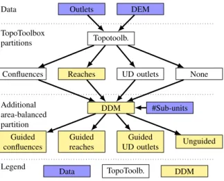
Data Outlets DEM
TopoToolbox
partitions Topotoolb.
Confluences Reaches UD outlets None
Additional area-balanced partition DDM #Sub-units Guided confluences Guided reaches Guided UD outlets Unguided Legend Data TopoToolb. DDM
Figure 3: Partitioning workflow.
The workflow is illustrated in Fig. 3. A preprocess is set up to read the DEM and user-defined points that rep-resent the outlets and engineered structures of interest. 3
In our case study, these are located near the pond out-lets. The partition, Fig. 4.a, is carried out with respect to these points using the TopoToolbox. This yields 6 sub-units corresponding to the 6 ponds, and a large sub-unit comprising the main stream.
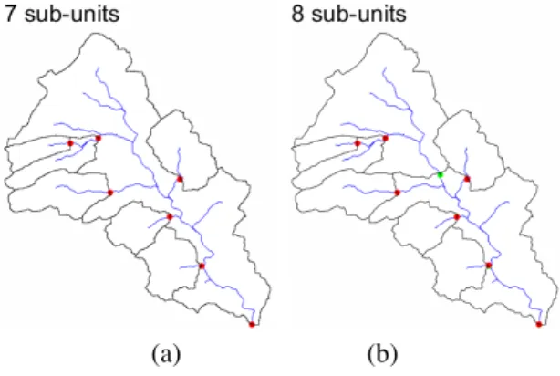
(a) (b)
Figure 4: Guided partitioning. a: User-defined points (red dots). b: Partition of the largest watershed into 2 sub-watersheds of similar area (green dot).
The area balancing watershed decomposition method is organized as follows. The sub-unit with largest area is selected and its flow accumulation information is com-puted. A cutting point is determined by searching for the cell that drains half of that flow, see Fig. 4.b. This process is iterated until the desired stopping criterion is met. This can be based on the number of sub-units and/or on the sub-unit areas.
In Fig. 4.b, the largest sub-unit of 58 km2 has been
split in two, one of 27 and one of 31 km2. Subsequent
partitions and their related characteristics are reported in Section 4.
The sub-watersheds are saved in the shapefile format using the shapewrite function of the Matlab Mapping toolbox such that it then can be used in the HEC-RAS simulations, for instance.
3.3. Improvements
Depending on the actual topography or its digitiza-tion, the watershed delineation may produce sub-units that present isolated cells, notably near to the outlet, see Fig. 5. Defects with respect to the 4-neighbor connec-tivity may occur for any partition method or partition software. These are not appropriate to a finite element modeling.
Thus, at the end of the partition process a connec-tivity check is performed to correct the decomposition by moving some of the outlet points upward. For each
Confluence method Unguided method
Ra
w
results
Corrected
Figure 5: Isolated cells near to outlets. Left: Partition method at con-fluences. Right: Unguided area balanced partition method.
sub-unit, this can be achieved by inspecting its proper-ties by means of the regionprops Matlab function, for instance.
3.4. Domain decomposition with HEC-RAS
The HEC-RAS version V-5 released in 2014 allows for 2D unsteady rain-on-grid simulations. The mini-mal data set comprises a DEM, the polygon delineat-ing the area of interest (shapefile, for instance), the boundary conditions, Manning’s roughness coefficient, and hydrological data (precipitation and/ or discharge). The HEC-RAS 2D, black-box, simulator comes with a sparse parallel solver for the solution of discrete flow equations on a multi-core processor.
HEC-RAS 2D is principally available for Windows and the the set-up of a multi-domain simulation remains challenging. In this paper, a proof of concept is pro-posed to evaluate the benefits of the domain decompo-sition method.
It is worth mentioning that HEC-RAS neither allows to delineate watersheds nor performs a partition at con-fluences in an automatic manner.
3.4.1. Workflow
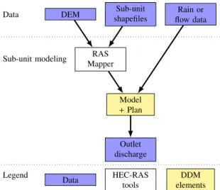
As shown in Fig. 6, the RAS Mapper interface is used to model the terrain starting from a DEM. Sub-unit shapefiles are imported to implement an area-balanced domain decomposition method. Then, corresponding 4
Data DEM shapefilesSub-unit Rain or flow data
Sub-unit modeling RAS
Mapper Model + Plan Outlet discharge Legend Data HEC-RAS tools DDM elements Figure 6: HEC-RAS workflow for a unique hydrological unit.
sub-units are meshed to discretize the partial di fferen-tial equations. A 1D river model is added at the sub-unit outlet, see subsection 3.4.2 below, so as to extract the flow hydrograph that serves as an input to the down-stream sub-unit.
The DDM sequence and the communications are au-tomated by means of a Virtual Basic Script (VBA) writ-ten using the HECRAS Controller functions, see sub-section 3.4.3 below. In this manner, the outflow of a sub-unit becomes the inflow of its downstream sub-unit.
Sequential computing (parallel-like) HECRAS-Controller VBA driver 2D–1D model+ Plan (1) Outlet discharge (1) 2D–1D model+ Plan (2) Outlet discharge (2) 2D–1D model+ Plan (3) Outlet discharge (3) Figure 7: DDM/HEC-RAS workflow.
3.4.2. 2D–1D modeling
The HECRAS Controller is initially designed to deal with 1D problems. Although it may run a 2D plan, it does not provide routines for the extraction of a 2D out-put information for now.
As proposed in [15], this shortcoming is addressed by adding a 1D model (river and cross sections) at the outlet of the 2D model of each of the sub-units. In that case, the HECRAS Controller function
OutputDSS GetStageFlow allows to derive the out-flow data of the sub-unit to be passed as inout-flow data to its downstream sub-unit.
As a downstream boundary condition, the 1D model makes use of the normal depth (slope) imposed on the most downstream cross-section of the 1D model.
Figure 8: 2D gridded flow area connected to a 1d river model with cross-sections
3.4.3. HECRAS Controller
The HECRAS Controller application programming interface [16] is designed to make transparent use of HEC-RAS 1D to drive a sequence of simulations.
In a nutshell, HECRAS Controller provides a collec-tion of routines that allows to open a project, to select and to run the so-called plans and to extract output data. These routines can be accessed in a number of in-terpreted programming languages, notably Visual Basic for Applications (VBA-in Excel).
The VBA script, see Fig. 7 organizes the computation sequence to account for the natural water flow. It runs sub-unit models from the most upstream to accumulate the stream flow at the watershed outlet. Each sub-unit calculation is carried out in one go, providing all the necessary input flow data to its downstream sub-unit.
The number of HEC-RAS plans corresponds to the number of sub-units.
4. Results
The performance of the confluence method and the area-balanced methods are compared on the generation of nested partitions, subsection 4.1, and the solution of 2D unsteady rain-on-grid simulations built for the Moderbach’s watershed, subsection 4.2. A discussion and an outlook are proposed in subsection 4.3.
Figure 9: Confluence partition method.
4.1. Nested partitions 4.1.1. Confluence method
In a watershed DEM, the stream network model is a set of connected segments, the number of which is parameterized by means of a threshold∆ on minimum drained cells, related to the minimum drained area in a straightforward manner. In the general case, stream confluences are connection points joining two upstream segments to one downstream segment. Consequently, the partition of a watershed at a unique confluence usu-ally yields two upstream sub-units and one downstream sub-unit.
The nested partitions plotted in Fig. 9 are produced with the thresholds reported in Tab. 2.
Properties Confluence partitions ∆ 20000 15000 9200 3100 #sub-units 3 5 9 23 Max. area 58.1 42.0 17.4 11.5 Min. area 13.6 4.9 0.4 0.2 Ratio 4.3 8.6 37.0 47.5 Mean area 29.7 17.8 9.9 3.8 Std dev. 24.9 14.2 5.6 2.7
Table 2: Characteristics of the confluence partitioning method. Area is expressed in km2.
As the number of confluences increases, there is an increasing probability for a very small sub-unit in the
partition. Consequently, the ratio between the maxi-mum and minimaxi-mum areas increases, too.
4.1.2. Guided area-balanced method
The guided method is carried out by starting from the 7 user-defined outlets that are located at the 6 pond out-lets and the watershed outlet. The generated sequence of nested partitions is illustrated in Fig. 10 and partition properties are reported in Tab. 3. The minimum area corresponds to the smaller sub-unit defined by a user points. Clearly, this strongly impacts the ratio between the maximum and minimum areas and the performance of the method. In the present case, the ratio decreases from 18.7 corresponding to the user-defined partition to 2.7 because the partitions into 7 and 8 sub-units involve very large sub-units.
Properties Partitions from user-defined points #sub-units 7 8 16 32 64 Max. area 57.9 27.4 7.6 3.9 2.0 Min. area 3.0 3.0 2.9 1.7 0.7 Ratio 19.3 9.1 2.6 2.3 2.9 Mean area 12 11.1 5.6 2.7 1.4 Std dev. 18.7 10.2 1.6 0.6 0.3
Table 3: Characteristics of the guided area-balanced partitioning method. Area is expressed in km2.
4.1.3. Unguided area-balanced method
The unguided method only requires the watershed outlet as an input. The nested partitions into a number of sub-units that is a powers of 2 are plotted in Fig. 11. Corresponding properties are reported in Table 4. This shows an increase of the ratio from 1.1 (the two sub-units have almost the same area) to approximately 2.9.
To summarize, the two area-balanced methods pro-vide similar performances when the number of sub-units is large. It should be mentioned that in these two methods, the minimum drained cells threshold ∆
Figure 10: Guided iterative area-balanced partition method.
Figure 11: Unguided iterative area-balanced partitioning method.
Properties Unguided partitions
#sub-units 2 4 8 16 32 64 Max. area 47.1 30.0 15.8 8.1 4.0 2.0 Min. area 42.1 17.1 8.1 3.8 2.0 0.7 Ratio 1.1 1.8 1.9 2.1 2.0 2.9 Mean area 44.6 22.3 11.1 5.6 2.8 1.4 Std dev. 3.5 5.5 2.7 1.3 0.6 0.3
Table 4: Characteristics of the unguided area balanced partitioning method. Area is expressed in km2.
is set to 1000 allowing to reach a large number of sub-units. The unguided method outperforms the confluence method in any case.
4.2. Domain decomposition 4.2.1. Numerical set-up
The HEC-RAS version 5.0.7 is used to model the hy-drological behavior of the Moderbach watershed. A precipitation event of 28 hours with an amount of 80 mm/day is imposed to saturate the watershed in a reasonable time. The remaining 44 h of the simulation are carried out with no precipitation in order to drain the watershed until reaching a null discharge at the main outlet.
This HEC-RAS version neglects infiltration, which supposes an quasi-impervious soil. Such a strong hy-pothesis is credible for this watershed in winter condi-tions. Manning’s coefficient is set to 0.03.
The boundary condition at the 1D river uses a normal depth estimated using the RAS Mapper. In our case, the slope parameter is about 0.001.
Runtimes were recorded in minutes on a Intel Xeon 64 bits @3.80 GHz×6 processor with 16 GB RAM memory. The sparse parallel solver of HEC-RAS makes use of the 6 cores of that processor.
4.2.2. Discharge results
Presented in Fig. 13(a).a are the discharge results computed at the outlet with HEC-RAS (workflow of
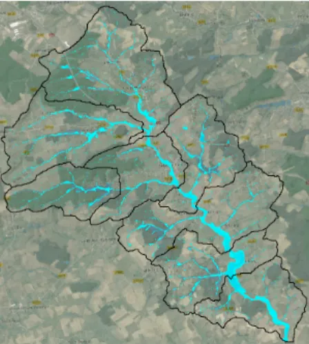
Figure 12: Flow extent generated from the simulation of the Moder-bach decomposed into 8 sub-units using unguided partition.
Fig. 6), and those obtained with the DDMs (workflow of Fig. 7) involving nested partitions of 2, 4 and 8 sub-units, respectively. Not shown are very similar results with the confluence partitioning method.
The relative errors displayed in Fig. 13(a).b exhibit very small discrepancies. These may be due to the value of the slope parameters or to topographical effects. In-deed, the partitioning methods may modify the hydro-logical behavior of the basin when a sub-unit outlet is located near to a dam, for instance.
4.2.3. Efficiency results
The computational efficiency of the DDM method is evaluated for a number of partitions carried out with re-spect to either the confluences or the (unguided) area balancing.
To evaluate the performances of the sparse parallel solver of HEC-RAS and the general behavior of the DDM, an overview of the computation times with re-spect to the sub-unit areas and the partition methods is provided in Fig. 14. In the graph, points of the same 7
(a) Discharge (b) Relative error
Figure 13: Main outlet flow computed using the unguided area-balanced partition. a: Discharge, b: Relative error evaluated with respect to the discharge computed on the total watershed.
Properties Unguided partitions #Sub-units 1 2 4 8 Max. time 183.0 70.3 45.4 20.1 Min. time 183.0 59.1 16.1 7.2 Ratio 1.0 1.2 2.8 2.8 Mean time 183.0 64.7 26.9 11.7 Std dev. - 7.9 13.1 4.7 Total time 183.0 129.4 107.6 93.9 Speed-up 1.0 1.4 1.7 2
Table 5: Computation time and speed up data for the DDM/HEC-RAS simulations of unguided partitions
color and of the same shape correspond to sub-units of the same partition. Triangles and filled circles are used to the unguided area-balanced partition method and the confluence partition method, respectively.
As expected, points are almost aligned in this log-log representation. The computation times and the ar-eas are linked by a power law, the slope of which re-flects the performance of the HEC-RAS sparse parallel solver. The differences in the solution times for the sub-units of very similar area indicate that the latter is a key parameter, but not the only one in this nonlinear solver. Moreover, Fig. 14 exhibits three colored clusters (filled circles of the area-balanced method) with very similar area and computing time. In contrast to that, the dispersion of the triangular points is much higher for the confluence method and very small sub-units are created. The main characteristics of these solution times are
Figure 14: Computation time per basin for the unguided area-balanced partition (triangles) and the confluence partition (filled circles).
presented in Tables 5 and 6.
The total time and the speedup are plotted, Fig. 15, against the number of sub-units. We see that for both partitioning methods, the decrease in computing time is multiplicative. For example, the times for the unguided balanced partition, Tab. 5, shows a speedup of 1.4 for the simulation of the configuration with 2 sub-units and 2 for 8 sub-units. For the confluence partition, Tab. 6, we have a speedup of 1.30 for 3 and 1.8 for 9 sub-units. As we have seen, the computation of the linear sys-tem generally grows super-linear in the size of the parts and thus with Jensen’s inequality [17] the sum of the 8
(a) times (b) speedup Figure 15: DDM–HEC-RAS computing times.
Properties Confluence partitions #Sub-units 1 3 5 9 Max. time 183.0 102.0 66.8 21.3 Min. time 183.0 17.1 4.7 0.8 Ratio 1.0 6.0 14.3 25.5 Mean time 183.0 47.1 24.3 11.1 Std dev. - 47.6 24.5 6.7 Total time 183.0 141.3 121.6 99.7 Speed-up 1.0 1.3 1.5 1.8
Table 6: Computation time and speed up data for the DDM/HEC-RAS simulations of confluence partitions
times of the linear systems of all parts is much smaller than for the linear system of the original watershed.
Additionally, Fig. 15 shows regressions of the form axb, where b is -0.27 and -0.32, respectively. This clearly shows the advantage of the partition method by a DDM in general, but also that the unguided balanced partition method improve the confluence method by an important factor.
4.3. Discussion
Even though hydrological data are considered as ho-mogeneous over the watershed in this paper, the DDM method allows to build simulation plans with homoge-neous data over the sub-units, but with heterogeneity over a large watershed. In particular, this may facili-tate the account for more actual precipitation and soil properties (Manning’s coefficient). Such heterogeneity is not considered here in order to carry out fair hydro-logical and methodohydro-logical comparisons.
A two-dimensional PDE solver is time and memory consuming, especially when the domain under study be-comes large. This applies to the two dimensional un-steady rain-on-grid solver recently proposed within the HEC-RAS software. Therein, linear systems are pro-cessed by a sparse parallel solver to take advantage of a multi-core processor.
This software is chosen to assess the benefits that could be brought by an additional partition of the wa-tershed into hydrological sub-units.
A number of watershed partitioning methods had been previously provided in the literature, for di ffer-ent purposes and following differffer-ent constraints (sec-tion 2.2) without, however, fully addressing the area balancing issue as demonstrated in Tab. 2. As demon-strated in Tabs. 3 and 4, both versions (user-guided or unguided) of our automated area-balanced partitioning method performs much better.
In particular, some user-defined outlets may be set to facilitate the account for civil engineering structural or topographical effects in the simulations. Then, comple-mentary outlets may be positioned in an automatic man-ner either at confluences or at points determined with respected to particular criteria. Finally, these allow to delineate sub-units with a similar area that can be used with a distributed hydrological model.
The impact of the improved balance in the sub-unit areas on the 2D PDE computation is assessed using HEC-RAS in Fig. 15 and Tab. 14. For our case study, the DDM workflow described in Figs. 6 and 7 results in a speed up of 2 when 8 sub units of similar size are sidered. Performances are a little lower with the con-fluence method. Simulatenously, the memory require-9
ments are also reduced.
For now, the VBA code developed using the HECRAS Controller functions allows to automate the DDM/HEC-RAS coupling strategy. The implementa-tion on a multi-processor cluster could bring an addi-tional reduction of the time to results. For the moment, this strongly depends on the maximum number of the sub-units in the upstream to downstream sequence.
Assuming the availability of the HEC-RAS sources, the DDM/HEC-RAS approach could benefit from two levels of parallelism. First, the sparse parallel solver of HEC-RAS performs the sub-unit computation on a multi-core processor. Second, the distribution of the sub-units on a multi-processor cluster may then further improve computing times.
5. Conclusion and outlook
As long as a certain balance between the tasks is maintained, domain decomposition together with par-allelization offer good opportunities for faster computa-tions that use larger data sets.
The GIS-based watershed partitioning methods we propose are based on an area-balancing criterion. They outperform the classical confluence and reach partition methods in the solution for the 2D unsteady rain-on-grid partial differential equations.
For general availability, the HEC-RAS software to-gether with the HECRASController tool have been cho-sen for the solution of the hydrological sub-problems, and the sequential implementation of a domain decom-position method.
Access to the internals of the software either by a pro-grammable API or by providing source code would be needed to go one step further. In that case, this DDM approach could provide two levels of parallelism to re-duce the computation time and to scale up the problem size. This would comprise a sparse parallel solver for the sub-unit computation on a multi-core processor, and the distribution of the sub-units on a core multi-processor cluster.
References
[1] F. M. Fan, W. Collischonn, K. Quiroz, M. Sorribas, D. Buar-que, V. Siqueira, Flood forecasting on the Tocantins River using ensemble rainfall forecasts and real-time satellite rainfall esti-mates, Journal of Flood Risk Management 9 (3) (2016) 278– 288.
[2] D. Falter, N. Dung, S. Vorogushyn, K. Schr¨oter, Y. Hundecha, H. Kreibich, H. Apel, F. Theisselmann, B. Merz, Continuous, large-scale simulation model for flood risk assessments: proof-of-concept, Journal of Flood Risk Management 9 (1) (2016) 3– 21.
[3] M. V. Sorribas, R. C. Paiva, J. M. Melack, J. M. Bravo, C. Jones, L. Carvalho, E. Beighley, B. Forsberg, M. H. Costa, Projec-tions of climate change effects on discharge and inundation in the Amazon basin, Climatic Change 136 (3-4) (2016) 555–570. [4] D. M. Bayer, W. Collischonn, Deforestation impacts on dis-charge of the Ji-Paran´a River–Brazilian Amazon, Climate and land surface changes in hydrology. 359th ed. Gothenburg: IAHS Publication H 1 (2013) 327–332.
[5] D. Yang, S. Herath, K. Musiake, Development of a
geomorphology-based hydrological model for large catchments, Proceedings of Hydraulic Engineering 42 (1998) 169–174. [6] F. Rodriguez, H. Andrieu, F. Morena, A distributed hydrological
model for urbanized areas–Model development and application to case studies, Journal of Hydrology 351 (3-4) (2008) 268–287. [7] G. Brunner, HEC-RAS River analysis system, 2D modeling user’s manual version 5.0, Davis: US Army Corps of Engineers, hydrologic engineering center .
[8] T. K. Apostolopoulos, K. P. Georgakakos, Parallel computation for streamflow prediction with distributed hydrologic models, Journal of Hydrology 197 (1-4) (1997) 1–24.
[9] E. R. Vivoni, G. Mascaro, S. Mniszewski, P. Fasel, E. P. Springer, V. Y. Ivanov, R. L. Bras, Real-world hydrologic as-sessment of a fully-distributed hydrological model in a parallel computing environment, Journal of Hydrology 409 (1-2) (2011) 483–496.
[10] P. R. M. Pontes, F. M. Fan, A. S. Fleischmann, R. C. D. de Paiva, D. C. Buarque, V. A. Siqueira, P. F. Jardim, M. V. Sor-ribas, W. Collischonn, MGB-IPH model for hydrological and hydraulic simulation of large floodplain river systems coupled with open source GIS, Environmental Modelling & Software 94 (2017) 1–20.
[11] W. Schwanghart, N. J. Kuhn, TopoToolbox: A set of Matlab functions for topographic analysis, Environmental Modelling & Software 25 (6) (2010) 770–781.
[12] V. A. Siqueira, A. Fleischmann, P. F. Jardim, F. M. Fan, W. Col-lischonn, IPH-Hydro Tools: a GIS coupled tool for water-shed topology acquisition in an open-source environment, Rbrh 21 (1) (2016) 274–287.
[13] M. Kumar, C. Duffy, Exploring the Role of Domain Partitioning on Efficiency of Parallel Distributed Hydrologic Model Simula-tions. J Hydrogeol Hydrol Eng 4: 1, of 12 (2015) 2.
[14] W. Schwanghart, D. Scherler, TopoToolbox 2–MATLAB-based software for topographic analysis and modeling in Earth surface sciences, Earth Surface Dynamics 2 (1) (2014) 1–7.
[15] C. Goodell, The HECRAS controller, a
power-ful feature of HEC-RAS exposed, retrieved from
https://www.icewarm.com.au/1, 2018.
[16] C. Goodell, Breaking the HEC-RAS Code: A User’s Guide to Automating HEC-RAS, H21s, 2014.
[17] J. L. W. V. Jensen, Sur les fonctions convexes et les in´egualit´es entre les valeurs Moyennes, Acta Mathemat-ica 30 (1) (1906) 175–193, doi:10.1007/bf02418571, URL https://doi.org/10.1007/bf02418571.
1https://www.icewarm.com.au/australian-water-school/
short-courses/course/powerful-hec-ras-features-exposed/