Impact of the 26-30 May 2003 solar events on the earth ionosphere and thermosphere.

(1)

HAL Id: hal-00155784

https://hal.archives-ouvertes.fr/hal-00155784

Submitted on 20 Dec 2015

HAL is a multi-disciplinary open access

archive for the deposit and dissemination of

sci-entific research documents, whether they are

pub-lished or not. The documents may come from

teaching and research institutions in France or

abroad, or from public or private research centers.

L’archive ouverte pluridisciplinaire HAL, est

destinée au dépôt et à la diffusion de documents

scientifiques de niveau recherche, publiés ou non,

émanant des établissements d’enseignement et de

recherche français ou étrangers, des laboratoires

publics ou privés.

Impact of the 26-30 May 2003 solar events on the earth

ionosphere and thermosphere.

Christian Hanuise, J.C. Cerisier, F. Auchere, K. Bocchialini, S. Bruinsma,

Nicole Cornilleau-Wehrlin, N. Jakowski, C. Lathuillere, Michel Menvielle, J.J.

Valette, et al.

To cite this version:

Christian Hanuise, J.C. Cerisier, F. Auchere, K. Bocchialini, S. Bruinsma, et al.. Impact of the 26-30

May 2003 solar events on the earth ionosphere and thermosphere.. Annales Geophysicae, European

Geosciences Union, 2006, 24 (1), pp.129-151. �10.5194/angeo-24-129-2006�. �hal-00155784�

(2)

Annales Geophysicae, 24, 129–151, 2006 SRef-ID: 1432-0576/ag/2006-24-129 © European Geosciences Union 2006

Annales

Geophysicae

From the Sun to the Earth: impact of the 27–28 May 2003 solar

events on the magnetosphere, ionosphere and thermosphere

C. Hanuise1, J. C. Cerisier2, F. Auch`ere3, K. Bocchialini3, S. Bruinsma4, N. Cornilleau-Wehrlin5, N. Jakowski6, C. Lathuill`ere7, M. Menvielle2, J.-J. Valette8, N. Vilmer9, J. Watermann10, and P. Yaya8

1_{LPCE/CNRS, 3A avenue de la Recherche Scientifique, 45071 Orléans Cedex, France} 2_{CETP/CNRS, 4 avenue de Neptune, 94107 St Maur des Fossés Cedex, France} 3_{IAS, Bâtiment 121, Université Paris Sud 11 – CNRS, 91405 Orsay Cedex, France} 4_{CNES, Département de Géodésie Spatiale, 31055 Toulouse Cedex 4, France} 5_{CETP/IPSL, 10-12 avenue de l’Europe, 78140 Vélizy-Villacoublay, France}

6_{Deutsches Zentrum für Luft und Raumfahrt, Kalkhorstweg 53, 17235 Neustrelitz, Germany} 7_{LPG, Bâtiment D de Physique, BP 53, 38041 St Martin d’Hères Cedex 9, France}

8_{CLS, 8-10 rue Herm`es, 31520 Ramonville Saint-Agne, France}

9_{LESIA, Observatoire de Paris, 5 place Jules Jansen, 92195 Meudon Cedex, France} 10_{Danish Meteorological Institute, Lyngbyvej 100, 2100 Copenhagen, Denmark}

Received: 23 February 2005 – Revised: 10 October 2005 – Accepted: 18 November 2005 – Published: 7 March 2006

Abstract. During the last week of May 2003, the solar

ac-tive region AR 10365 produced a large number of flares, sev-eral of which were accompanied by Coronal Mass Ejections (CME). Specifically on 27 and 28 May three halo CMEs were observed which had a significant impact on geospace. On 29 May, upon their arrival at the L1 point, in front of the Earth’s magnetosphere, two interplanetary shocks and two additional solar wind pressure pulses were recorded by the ACE spacecraft. The interplanetary magnetic field data showed the clear signature of a magnetic cloud passing ACE. In the wake of the successive increases in solar wind pres-sure, the magnetosphere became strongly compressed and the sub-solar magnetopause moved inside five Earth radii. At low altitudes the increased energy input to the magne-tosphere was responsible for a substantial enhancement of Region-1 field-aligned currents. The ionospheric Hall cur-rents also intensified and the entire high-latitude current sys-tem moved equatorward by about 10◦. Several substorms occurred during this period, some of them – but not all – apparently triggered by the solar wind pressure pulses. The storm’s most notable consequences on geospace, including space weather effects, were (1) the expansion of the auro-ral oval, and aurorae seen at mid latitudes, (2) the significant modification of the total electron content in the sunlight high-latitude ionosphere, (3) the perturbation of radio-wave propa-gation manifested by HF blackouts and increased GPS signal scintillation, and (4) the heating of the thermosphere, causing

Correspondence to: C. Hanuise

([email protected])

increased satellite drag. We discuss the reasons why the May 2003 storm is less intense than the October–November 2003 storms, although several indicators reach similar intensities.

Keywords. Interplanetary physics (Solar wind plasma) –

Magnetospheric physics (Magnetosphere-ionosphere inter-actions), Ionosphere (Ionosphere-atmosphere interactions)

1 Introduction

Geospace is at all times affected by the solar wind, a super-sonic plasma stream emerging from the Sun. Besides large-scale recurrent structures (such as the interplanetary mag-netic field sector and solar wind flow regime boundaries), eruptive solar events of high intensity, predominantly solar flares resulting in halo Coronal Mass Ejections (CMEs) and solar energetic particle emissions, can have a significant im-pact on geospace. The vast majority of the very intense storms were observed to be associated with interplanetary CMEs (ICMEs) and shocks passing by the Earth (Tsuru-tani and Gonzalez, 1997). They are an interplanetary man-ifestation of earthward directed CMEs. If the Earth is in a favourable position with respect to the solar source of a CME, it may deposit large amounts of energy in the Earth’s magnetosphere. A part of it is released immediately while another part is stored in the magnetosphere and released later. Such solar events follow a causal chain in the sense that there is always a solar source where the disturbances orig-inate and from where they propagate through interplanetary space and eventually interact with the Earth’s magnetosphere

(3)

130 C. Hanuise et al.: Impact of the 27–28 May 2003 solar events

Fig. 1. Left: Magnetogram of the solar disk obtained with MDI/SOHO on 24 May 2003 at 9:36 UT. Active Region AR 10365 is indicated by the orange square. Right: 140×110 arcsec2 im-age centred on AR 10365 observed with THEMIS on 27 May at 06:58 UT in Fe I 630.2 nm.

to initiate magnetospheric and ionospheric storms. After propagation through the interplanetary space, it is the config-uration of the solar wind plasma (density and bulk velocity) and magnetic field (intensity and direction) at the Earth’s lo-cation which determines the strength of the interaction with the magnetosphere. The consequences of such storms can be noticed immediately (e.g. auroral displays, large variations of the geomagnetic field) and may adversely affect humans and technological systems (e.g. enhanced radiation, disturbed ra-dio wave propagation). However, the various links of this chain – from the Sun to the resulting space weather effects – are often treated separately and independently, due to the fact that they fall into the realms of different research com-munities.

In this paper, we make an attempt to study the entire chain for a short sequence of individual (though complex) solar and geospace events. To do so we have selected the 27–30 May 2003 space storm period during the declining phase of solar cycle 23, which was characterized by numerous solar flares and several Earth directed CMEs, resulting in an “intense ge-omagnetic storm” (minimum Dst=–131 nT), according to the

classification of Gonzalez et al. (1994).

We give a comprehensive description of the physical pro-cesses associated with this period of solar activity, start-ing with the energy release at the solar surface and end-ing with the energy deposition in geospace and the associ-ated space weather effects on technological systems. To do so, it proves to be essential to collect data from a number of platforms, notably the SOHO and ACE spacecraft at the L1 point, as well as the GOES and CLUSTER satellites, but also from a number of ground-based observatories and other measurement sites. The May activity occurred during the 11th MEDOC (Multi-Experiment Data and Operation Cen-tre) campaign, during which intensive SOHO observations were undertaken in coordination with the EISCAT/ESR and SuperDARN radars.

Section 2 deals with the solar activity observed during the 26–28 May period when the active region AR 10365 was the source of several X class flares and associated CMEs. Section 3 first summarizes solar wind conditions as observed

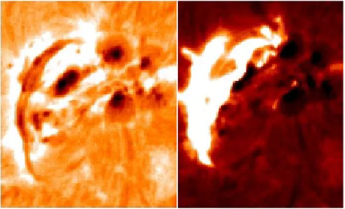
Fig. 2. Left: Hα image of AR 10365 on 27 May 2003 at 22:46:26 UT; 15 min before the first observation of the CME. Fila-ment and pores are visible. The field of view is 250×300 arcsec2. Right: Same field of view at 23:06:26 UT, at the appearance of the flare; the filament has disappeared (images from Big Bear Solar Ob-servatory).

by ACE before analysing the propagation of the halo CMEs through the interplanetary medium. In Sect. 4, the global impact of the CMEs on the magnetosphere is evaluated, both through its compression by the increased solar wind pressure and through the increased energy input which oc-curred mainly during the periods of large southward inter-planetary magnetic field (IMF), favouring reconnection at the magnetopause. The electrodynamic response of the coupled magnetosphere-ionosphere system to the various phases of the storm is described in Sect. 5, based on magnetic (the latitudinal chains in Greenland and Scandinavia and mag-netic indices) and incoherent scatter radar (EISCAT) mea-surements. Thereafter, we focus in Sect. 6 on the conse-quences of the storm on the neutral and ionized components of the atmosphere (thermosphere and ionosphere, respec-tively). We conclude the description of the event in Sect. 7 with a more practically oriented assessment of several of the storm effects on the near-Earth environment (space weather effects), with emphasis placed on the absorption of High Fre-quency (HF) waves in the lower ionosphere, the perturbation of low-altitude satellite orbits due to increased atmospheric drag and ionospheric scintillations in the radio signals of the Global Positioning System (GPS) due to plasma turbulence. Finally Sect. 8 discusses the observations in a comparative context with the larger storms of the October (Halloween) and November 2003 periods.

2 The solar Active Region AR 10365

The combination of ground-based and space-borne solar ob-servations provides the opportunity to follow the time evolu-tion of the active region AR 10365 from the photosphere up to the corona. According to NOAA/SEC reports, more than 30 flares occurred in AR 10365 from 26 May at 00:00 UT until 29 May at 00:00 UT; the magnetic fluxes increased and reached their maximum on 28 May (1.2×1014Tesla m2on

(4)

C. Hanuise et al.: Impact of the 27–28 May 2003 solar events 131 EIT 304: 1998 May 27 - 23:12 - 22:36 EIT 304: 1998 May 27 - 23:12 EIT 304: 1998 May 27 - 23:59 - 23:47 EIT 304: 1998 May 28 - 00:36 - 00:24 EIT 304: 1998 May 28 - 00:24 - 00:11 LASCO C2: 1998 May 28 - 00:50 - 00:42 1st EIT wave front

2nd EIT wave front 1st Halo front

2nd Halo front

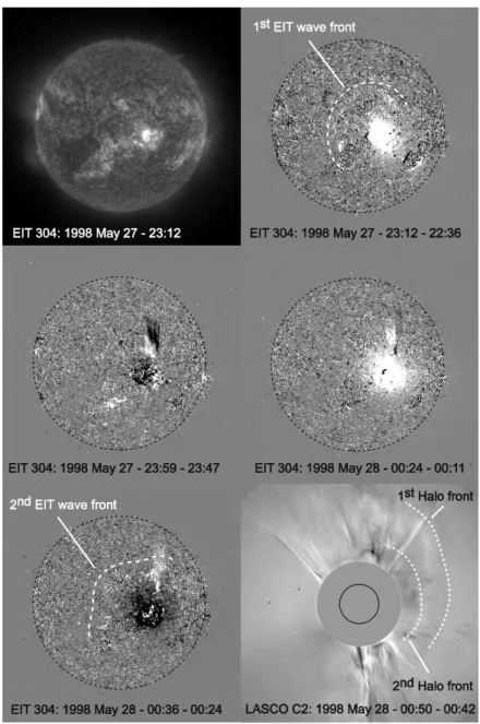
Fig. 3. SOHO observations. The top left image is the Sun seen by EIT in the 30.4 nm line of He II. AR10365 is defined by the strong intensity

enhancement. The 4 following images are EIT running difference at 30.4 nm (He II); the first flare is detected by EIT at 23:12 UT on 27 May 2003 (top right), and the second at 00:24 UT on 28 May 2003 (centre right). The centre left image shows a black and white structure at the north of the AR: this is the signature of the ejected filament seen on Fig. 2. On the bottom left and top right images, the white dotted lines indicate the circular front propagating from the centre of the AR, and associated to EIT waves seen in projection on the solar disk. The bottom right image shows the 2 halo CMEs seen by LASCO-C2/SOHO on 28 May between 00:50 UT and 00:42 UT (running difference). The position of the Sun is indicated by the black circle. The grey disk is the mask of the coronagraph occulting the Sun.

the average), i.e. 4.5 days after the emerging flux birth (Chae et al., 2004). These authors suggest that the largest flare ex-plosion may have been related to the accumulation of mag-netic helicity in the corona and noted that “the strongest flare occurred after the rate of helicity injection peaked”.

At the photospheric level, MDI/SOHO (Scherrer et al., 1995) magnetograms obtained between 20 May and 29 May 2003 showed a complex magnetic structure in AR 10365 (in-dicated by an orange square in Fig. 1, left panel), with sev-eral inversion lines. This complex structure is confirmed by

the high resolution magnetogram obtained in the Fe I line at 630.2 nm at the THEMIS observatory on 27 May at 06:58 UT (Fig. 1, right). MDI magnetograms show an emerging flux which appeared on 24 May around 09:36 UT, east of the ac-tive region, and grew until it became as large as the initial active region itself.

At the chromospheric level, an Hα image obtained on 27 May at 22:46 UT from Big Bear Solar Observatory re-veals a few small black circular structures known as pores (also seen on Fig. 1, right) and a black elongated structure on

(5)

Table 1. Characteristics of the 3 halo CMEs observed on 27–28 May 2003.

CME 1 CME 2 CME 3

Date / Time May 27, 2003 @ 06:50 UT May 27, 2003 @ 23:50 UT May 28, 2003 @ 00:50 UT

Speed (*) 509 km/s 960 km/s 1370 km/s

Associated Flare M1.6 @ 06:26 UT X1.3 @23:07 UT X3.6 @00:27 UT

(*) speed estimates at 20 Rs derived from the measurements of the CMEs by C2 and C3 coronagraphs

Table 1: Characteristics of the 3 halo CMEs observed on May 27-28, 2003.

Satellite date UT X (R/Re) Y (R/Re) Z (R/Re) d_sibeck(Re)

GOES 10 29/05/2003 19:00 5.49 -3.14 0.94 6.3

C1 29/05/2003 22:00 -3.47 -4.84 -9.59 6.6

C2 30/05/2003 00:12 -2.67 -1.29 -8.15 5.1

C4 30/05/2003 00:20 -3.05 -2.30 -8.05 5.0

Table 2: Location of the magnetopause crossings and estimated radial distance of the

subsolar point according to the model of Sibeck et al. (1991).

Day / Time UT Event Observed in

29 / 12:25 Interplanetary shock - Sudden Impulse ACE data, SYM-H

29 / 13:50 Substorm AE, ASY-H

29 / 16:10 Pressure pulse & Substorm ACE data, AE, ASY-H 29 / 19:06 Interplanetary shock - Sudden Impulse

Substorm

ACE data, AE, ASY-H

30 / 01:50 Bz northward ACE data

Table 3: Chronology of interplanetary (ACE), magnetospheric and ionospheric events

Storms /2003 May 29 October 29 October 31 November 20 Storm intensity:

Minimum Dst (nT) -130 -363 -401 -472

Source Flare Intensity X3.6 X17.2 X11 M3.2

Magnetic cloud at ACE

Fig. 4. X-ray flux recorded by GOES between 26 May 00:00 UT and 29 May 00:00 UT: two peaks of x-ray flux occur on 27 May around

23:10 and on 28 May around 00:30 UT, respectively.

the left which could be an active filament (Fig. 2, left). Fig-ure 2 (right) shows the active region at 23:05 UT at its inten-sity maximum, probably indicating the beginning of the X1.2 flare observed at 23:10 UT by the GOES-10 and GOES-12 satellites.

On 27–29 May 2003 the EUV Imaging Telescope (EIT, Delaboudini`ere et al., 1995) on board SOHO was in “CME watch” mode (12-min cadence), in the 30.4-nm line of He II (formed in the chromosphere to corona transition region at 0.8 MK). This mode allows the observation of the initial phase of CMEs. The CMEs are initiated in association with flares and/or prominences/ filament ejections (Delann´ee et al., 2000), and are the consequence of global instabilities of the magnetic field (Schmieder et al., 2002). The “CME watch” mode is usually operated in the 19.5-nm wavelength band of Fe XII (formed in the hot corona at 1.5 MK). Thomp-son et al. (1999) analysed EIT image differences in Fe XII and showed, for the first time, waves in expansion from the initiation site of the halo CME. These waves are a signature of halo CMEs and represent globally propagating coronal disturbances which emanate from a central radial point and travel across the visible solar surface (Gilbert et al., 2004). In

their MHD simulations, Chen et al. (2005) demonstrate that EIT waves are thought to be formed by successive stretch-ing or openstretch-ing of closed field lines driven by an eruptstretch-ing flux rope: “during the stretching process, the plasma on the outer side of the field line is compressed to form the density-enhanced EIT wave front, while inside the field line, the plasma is evacuated to form a dimming region due to the expansion”. The propagation speed of the waves is typically around 250 km/s but has been observed to reach 800 km/s (Zhukov and Auch`ere, 2004). The relations between flares, prominence ejections and CMEs are, however, difficult to es-tablish observationally.

The He II movie for 27–29 May 2003 shows two succes-sive intensity enhancements (flare signature) in AR 10365 at 23:12 UT on 27 May and at 00:24 UT on 28 May 2003. In the former case the flux increase is about 15% but due to telemetry limitations, the very beginning of the CME at 23:10 UT was not recorded; in the latter the flux increase is about 20%. Simultaneously with the first enhancement, the filament described in the Hα image in Fig. 2 is ejected in the northwest direction (projected on the disk), and ap-pears as dark material absorbing the He II radiation. Figure 3

(6)

C. Hanuise et al.: Impact of the 27–28 May 2003 solar events 133

ACE IMF (GSM) / SW * 2003/05/27-30 No Delay

27/05/03 28/05/03 29/05/03 30/05/03 Time, UT 00 06 12 18 00 06 12 18 00 06 12 18 00 06 12 18 00 0 20 40 0 0 -20 20 104 105 20 40 500 700 800 600 | |B Bz Np Vel Tp B_imf ,nT Bz_imf ,nT Density ,c m-3 SW speed, km/s T protons, K P C I R P C I R IS IS

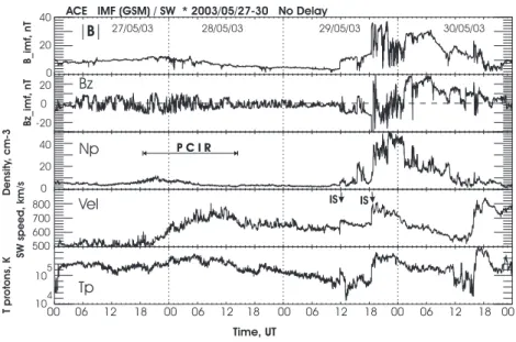
Fig. 5. IMF and solar wind parameters at L1 for the period 27–30 May 2003 recorded by the ACE spacecraft.

contains a series of running difference images in He II. On images 2 to 5, we clearly see the cold ejected material (black and white structure) coming from the erupting filament, at the top of AR 10365. After each flare, we can see the pro-gression of a faint halo, centred on the AR and associated with waves, the disk projection of which were observed by EIT; in both cases, the circular wave fronts are propagat-ing at an exceptionally large speed of 1000 km/s, larger than the usual EIT waves. Signatures of the events described above were also recorded by the Large Angle and Spectro-metric Coronograph (LASCO) on board SOHO. The list of CMEs observed by LASCO (Brueckner et al., 1995) and published at http://cdaw.gsfc.nasa.gov/CME list/ shows that up to ten CMEs were observed with the C2 coronagraph be-tween 01:50 UT on 27 May and 00:50 UT on 28 May. As described, for example, in Vilmer et al. (2003), halo CMEs have a higher probability to reach the Earth’s orbit. Table 1 gives the time of appearance of the three 27 May–28 May halo CMEs observed in C2, their estimated speed and the associated flares, as observed by GOES (Fig. 4). In the fol-lowing sections, we determine the signatures and investigate the effects of these 3 halo CMEs in geospace.

3 Solar wind/interplanetary conditions

ACE observations at L1 for the period 27 May to 30 May are shown in Fig. 5. The perturbed period started to be observed by ACE in the evening of 27 May when a Pseudo Corotating Interaction Region (PCIR) (Tsurutani et al., 1995; Gonzalez et al., 1999) was observed, as indicated by (i) a smooth solar wind density increase followed by a decrease from a maxi-mum of 10 cm−3at 21:30 UT on 27 May, (ii) a solar wind ve-locity maximum larger than 600 km/s around 10:00 UT, and (iii) a solar wind temperature increase up to 5×105K. The PCIR is probably the signature of the Earth entering a coronal

hole stream which is characterized by enhanced background solar wind speed. It was followed, on 29 May, by the arrival of two interplanetary shocks (IP), as indicated by vertical ar-rows in Fig. 5, shortly before noon and around 18:30 UT. In each of these shocks, the density and the bulk velocity of the solar wind increase substantially, up to 40 cm−3 and 800 km/s after the second shock.

The interplanetary magnetic field displays a complex structure. After each of the two shocks, the IMF exhibits one classical magnetic cloud behaviour with an increase in the amplitude and an inversion of Bz usually attributed to a flux rope structure. The minimum Bz reaches –30 nT at the arrival of the second shock. Later, Bz retreats to less extreme values before turning northward in the early hours of 30 May. The magnetic clouds and shocks are now related to their solar origin (CMEs and flares), using the procedure described in Vilmer et al. (2003). An early limit to the launch time is estimated assuming that the interplanetary perturbation prop-agates with a constant velocity, given by the value measured at 1 AU. Shortly after the first shock, the velocity is of the or-der of 700 km/s, leading to a transit time of two days and ten hours from the Sun to ACE. The launch window thus starts at 01:50 UT on 27 May. It is very likely that the first interplan-etary CME (ICME) is associated with the first halo CME at 06:50 UT (transit time of two days and five hours), and that the second shock and subsequent magnetic cloud is associ-ated with a combination of the two very fast halo CMEs, with the later one probably catching up with the earlier one. This is consistent with previous findings for a series of interplan-etary perturbations and a series of fast halo CMEs (Vilmer et al., 2003). As suggested in previous studies, the perturbation does not propagate with a constant speed between the Sun and the Earth (Gopalswamy et al., 2000; St. Cyr et al., 2000). CMEs are likely to interact with the often-slower ambient solar wind. It is thus expected and it has been observed that the speed of most ICMEs has decreased down to that of the

(7)

134 C. Hanuise et al.: Impact of the 27–28 May 2003 solar events 2003/05/29 2003/05/30 06 12 18 00 06 AE inde x 0 1000 2000 06 12 18 00 06 Time, UT 06 12 18 00 06 2003/05/30 0 20 30 0 0 -20 20 20 40 By_imf ,nT Bz_imf ,nT SW pressure, nP a 50 30 10

ACE IMF (GSM) / SW * 2003/05/29 Delay 36 min

-20 SYM H AS Y H

SYM-H ASY-H INDICES * 2003/05/29-30

2003/05/29 2003/05/30

PP

SO

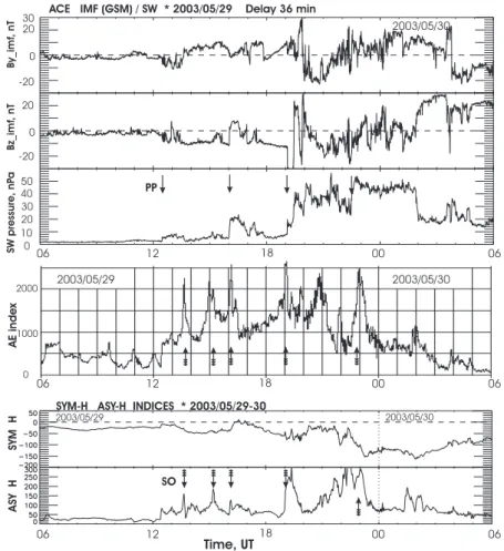
Fig. 6. Characterization of the main phase of the magnetic storm. Top: IMF and solar wind pressure derived from ACE observations. Time

is delayed by 36 min in order to match magnetospheric data. Centre: Auroral Electrojet (AE) index. Bottom: SYM-H and ASY-H indices.

solar wind at the ACE location. This appears to be the case for the two fast halo CMEs of 27–28 May.

4 Solar wind – magnetosphere coupling

Let us now focus on the period following the arrival of the first shock around 12:00 UT on 29 May. ACE data for the 30-h period starting on 29 May at 06:00 UT are displayed in Fig. 6 (upper panel). The measured solar wind speed sug-gests that the delay from ACE to the dayside magnetosphere boundary varies between 33 and 41 min during that period. Thus, for easier comparison with magnetospheric data, the ACE data in Fig. 5 have been delayed by a mean transit time to the magnetosphere of 36 min. We will refer to this delayed time further in this paper.

During the initial period of the magnetic cloud passage, from 12:28 UT on 29 May until 01:53 UT on 30 May, the IMF Bz is negative (with several short positive excursions), reaching a minimum value of –32 nT after 19:00 UT. In ad-dition to the two interplanetary shocks mentioned in the pre-vious section, which are assumed to have arrived at the mag-netopause at 12:28 UT and 19:06 UT, respectively, the so-lar wind pressure shows two increases associated with den-sity jumps at 16:00 UT and 22:30 UT (estimated arrival).

These four dynamic pressure pulses (PP as indicated by ver-tical arrows) are responsible for the sudden impulses or storm sudden commencements (SSC) recorded by various ground magnetometers. The second shock (third pulse) is followed by a long period (about 7 h) of very high pressure (oscillating between 30 and 50 nP). At 01:53 UT on 30 May, the IMF Bz turns positive and persists.

4.1 Magnetosphere compression

The influence of the solar wind pressure changes on the size of the magnetosphere can be inferred from GOES-10/12 and Cluster observations. Energetic particle and magnetic field measurements aboard GOES-10 and GOES-12 indicate that the magnetopause moved inside the geosynchronous orbit at 19:00 UT on 29 May upon the arrival of the second inter-planetary shock. Later, Cluster, on its inbound path, left the magnetosheath and entered the compressed magnetosphere in the early morning sector, as indicated by characteristic changes in the dynamic frequency spectra of the magnetic ULF turbulence and of the magnetic field component per-pendicular to the spin plane (Fig. 7, top panels from the STAFF experiment, Cornilleau-Wehrlin et al., 2003). The magnetosheath populated by solar wind shocked particles is

(8)

C. Hanuise et al.: Impact of the 27–28 May 2003 solar events 135 2003 May 29, 18:00 to 2003 May 30, 01:00 Bo w s ho ck mo de l CLUSTE R 4 CLUSTE R 1 Mag neto paus e m odel 10 20 0 0 10 -10 -20 X (R )_GSE E R = ( Y + Z ) (R ) E GS E 2 2 1/ 2 20 G OE S 1 0

Fig. 7. Magnetopause crossings observed by different spacecraft. Top panels: Cluster-STAFF ULF dynamic spectra and magnetic field

modulus in the spin plane around magnetopause crossings for spacecraft 1 and 4. The lower panel shows the orbit of GOES 10, CLUSTER 1 and CLUSTER 4 in x, (y2+z2)1/2GSE coordinates for the 18:00–01:00 UT time interval. The orbits are represented by the green, red and blue arrows, respectively. The magnetopause position deduced from its crossing by those 3 spacecraft is drawn with the same colour code (see Table 2). The mean magnetopause and bow shock for quiet solar wind conditions (PSW=2.1 nPa, IMF Bz=0) are shown in black for comparison.

characterized by intense, quasi-permanent, ULF, broad-band emissions, whereas only weak, quasi-monochromatic emis-sions are observed in the outer magnetosphere. A sudden decrease in the electron flux intensity in the sub-KeV energy range (typical magnetosheath population) confirms the en-trance of Cluster into the outer magnetosphere (PEACE ex-periment, Johnstone et al., 1997; D. Fontaine, private com-munication). According to the magnetopause model used for orbit prediction under moderate solar wind conditions

(pressure=2.1 nP, IMF Bz=0), Cluster 1, which was the most earthward of the four spacecraft, should have entered the magnetosphere on the dawn side around 12:00 UT on its in-bound path. However, it remained in the magnetosheath up to 22:00 UT and even made two excursions into the unshocked solar wind. Cluster 1, 2 and 4 entered the magnetosphere at 22:00 UT on 29 May and at 00:12 UT and 00:20 UT on 30 May, respectively, as shown on Fig. 7 (bottom panel, only spacecraft 1 and 4).

(9)

Table 2. Location of the magnetopause crossings and estimated radial distance of the subsolar point according to the model of Sibeck et

al. (1991).

CME 1 CME 2 CME 3

Speed (*) 509 km/s 960 km/s 1370 km/s

Satellite date UT X (R/Re) Y (R/Re) Z (R/Re) d_sibeck(Re)

GOES 10 29/05/2003 19:00 5.49 -3.14 0.94 6.3

C1 29/05/2003 22:00 -3.47 -4.84 -9.59 6.6

C2 30/05/2003 00:12 -2.67 -1.29 -8.15 5.1

C4 30/05/2003 00:20 -3.05 -2.30 -8.05 5.0

Substorm

ACE data, AE, ASY-H

Storms /2003 May 29 October 29 October 31 November 20 Storm intensity:

Minimum Dst (nT) -130 -363 -401 -472

Fig. 8. R-1 current in the 15:00–16:00 MLT sector derived from

CHAMP magnetometer data. Top: Current intensity (latitudinally integrated current density). Centre: Latitudinal position of the equa-torward (solid) and poleward (dashed) boundaries of the R-1 current sheet. Bottom: Polar Cap North (P CN ) index.

From the measured location of the magnetopause cross-ing, it is possible to derive the geocentric distance of the magnetopause subsolar point with the help of the Sibeck et al. (1991) model. The values are given in the last column of Table 2. It is obvious that the compression has increased with time. The estimated subsolar distance was close to 6.5 RE

(Earth radii) around 19:00 and 22:00 UT on 29 May and 5 REat 00:20 UT on 30 May, in response to the

correspond-ing increase in the solar wind pressure. The bottom panel of Fig. 7 displays the orbits of Cluster 1 and 4 and GOES-10, together with the position of the magnetopause inferred from the crossing times and from the Sibeck et al. (1991) model. 4.2 Energy input to the magnetosphere

Several indicators of the coupling of the interplanetary medium with the magnetosphere have been proposed (Gon-zalez et al., 1989 and references therein). Computed from solar wind parameters, generally observed at L1, they aim at characterizing and monitoring the energy transfer from the solar wind to the magnetosphere. The solar wind

cou-pling to the magnetosphere and ionosphere, and the associ-ated energy transfer can also be evaluassoci-ated directly from the dayside Region-1 (R-1) field-aligned currents (FAC). Ijima and Potemra (1982) have quantified the relationship between these R-1 current densities and the interplanetary parameters. We have deduced the FAC density from magnetic field measurements collected from 29 May at 06:00 UT, until 30 May at 12:00 UT, by the low-altitude polar orbiting CHAMP satellite (Reigber et al., 1999). During this period, the satellite crossed the northern auroral ionosphere in the early-afternoon (15:00–16:00 MLT) sector. Figure 8 shows estimates of the R-1 current obtained by integration of the FAC density over its full latitudinal extent. The R-1 current exceeds 0.7 A/m for 12 successive passes, from 13:15 UT on 29 May until 06:10 UT on 30 May. This period encompasses the passage of the magnetic cloud. The maximum value of 3.5 A/m is observed during the 22:20 UT pass on 29 May at the time of maximum solar wind pressure associated with the largest negative IMF Bz. This value is more than 10 times the typical quiet time value of 0.25 A/m (Potemra, 1994). The northward turning of the IMF is followed by a strong decrease in the R-1 current, down to 1 A/m, a value signif-icantly larger than the pre-storm value (0.5 A/m). This per-sisting R-1 current may be attributed to the perper-sisting high solar wind pressure. Similar observations have been made by Le et al. (1998) during a period of positive Bz and high solar wind pressure following the January 1997 storm, where the R1 current was observed to remain at twice its pre-storm intensity. The solar wind pressure has also been shown to correlate positively with the intensity of the auroral electro-jets for positive Bz (Shue and Kamide, 2001).

Our observations demonstrate that although the negative

Bz is the dominant factor controlling the energy input to

the magnetosphere, the large solar wind pressure also plays an important role, even during periods of positive Bz. In their analysis of the northward IMF period following the 22–24 October 2003 magnetic cloud, Øieroset et al. (2005) observed a gradual transition to a cold and dense plasma sheet, together with reversed ion dispersion signatures in the cusp, indicative of reconnection poleward of cusp. These ob-servations agree with a global MHD simulation (Li et al., 2005), in which magnetosheath plasma entering the magne-tosphere poleward of the cusp is convected to the tail. It has also been shown by Feldstein et al. (1984) that finite ener-gization of the ring current still occurs for positive Bz.

(10)

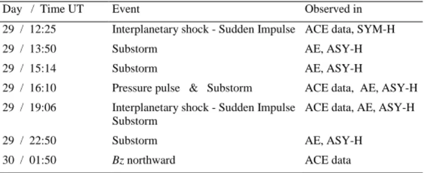
Table 3. Chronology of interplanetary (ACE), magnetospheric and ionospheric events.

CME 1 CME 2 CME 3

Speed (*) 509 km/s 960 km/s 1370 km/s

Satellite date UT X (R/Re) Y (R/Re) Z (R/Re) d_sibeck(Re) GOES 10 29/05/2003 19:00 5.49 -3.14 0.94 6.3

C1 29/05/2003 22:00 -3.47 -4.84 -9.59 6.6 C2 30/05/2003 00:12 -2.67 -1.29 -8.15 5.1 C4 30/05/2003 00:20 -3.05 -2.30 -8.05 5.0

Substorm

ACE data, AE, ASY-H

Storms /2003 May 29 October 29 October 31 November 20

Storm intensity:

Minimum Dst (nT) -130 -363 -401 -472

Both the negative IMF Bz and the high solar wind pressure are responsible for the equatorward motion of the R-1 current by as much as 10◦–12◦(Fig. 8, centre panel). During the pos-itive Bz period after 02:00 UT on 30 May, a strong downward current (the northward Bz or NBZ current, Ijima et al., 1984) is observed poleward of the R-1 current. This NBZ current is also a manifestation of solar wind-magnetosphere cou-pling, due to reconnection occurring poleward of the mag-netospheric cusps.

5 Magnetosphere – ionosphere coupling

5.1 Parameters characterizing the state of the magneto-sphere – ionomagneto-sphere current system

Geomagnetic indices can be used to monitor and character-ize the global response of the magnetosphere-ionosphere sys-tem. They are computed from geomagnetic field variations recorded at ground-based observatories, and most of them constitute data series which are homogeneous over the four latest solar cycles. SuperDARN radars are another powerful means of monitoring the magnetospheric and ionospheric re-sponses by mapping the plasma convection over the whole polar cap. Unfortunately, data are usually unavailable dur-ing very intense magnetic storms, due mainly to increased absorption of HF radio waves in the D region. This was in-deed the case on 29 May (see Sect. 7.1). Therefore, we have chosen to describe magnetospheric and auroral activity at a global level using the P CN , AE, Dst, SYM-H and ASY-H

geomagnetic indices.

The Polar Cap (PC) magnetic index has been proposed by Troshichev et al. (1979, 1988). It is based on a statistical analysis of the relationship between the solar wind merg-ing electric field and the magnetic disturbances observed at near-pole stations, one in each hemisphere. We only consider here the northern PC index (P CN ). It is representative for the magnitude of the northern trans-polar convection elec-tric field which drives the transpolar part of the ionospheric two-cell DP2 current system. As a result, increasing P CN values can be interpreted as increasing dayside merging, as indicated by the good correlation between the R-1 current and the P CN index shown in Fig. 8 (bottom panel).

The auroral activity indices (AE, AU , AL, A0, classically referred to as AE indices or simply AE) have been intro-duced by Davis and Sugiura (1966). They are at present based on the transient variations in the geomagnetic north component observed at a network of 11 observatories dis-tributed in longitude over the auroral oval. AE monitors the magnetic activity produced by enhanced ionospheric currents in the auroral zone, mostly related to the magnetosphere-ionosphere coupling through the field-aligned currents. It is worth noting that AE stations are located at standard au-roral oval latitudes. They may fail to properly capture the magnetic signature of the auroral phenomena during periods of intense geomagnetic activity, as a result of the associated equatorward motion of the auroral oval. As will be shown in the following section, this happens during some periods of the event we consider here.

The Dst, derived on a 1-h basis, measures the variations

in the geomagnetic north component at four low-latitude ob-servatories (Sugiura, 1965; Sugiura and Kamei, 1991). It monitors the axi-symmetric part of the magnetospheric cur-rents, including mainly the ring current, but also the mag-netopause Chapman-Ferraro current. The SYM-H index is essentially the same as Sugiura’s hourly Dst index, but with

the advantage of being derived on a 1-min basis and from a different set of stations. The ASY-H index measures both the direct and the unloading response of the magnetosphere (partial ring current). In particular, the signature of substorm onsets takes the form of a sharp positive peak in ASY-H and in AE. In the present study, we use SYM-H (one-minute time resolution) or Dst (1-h time resolution), depending on

the context. The time histories of the indices are displayed in the lower panels of Fig. 6 for AE, SYM-H and ASY-H, and in Fig. 8 for P CN .

5.2 Electrodynamics of the magnetosphere-ionosphere sys-tem

Table 3 lists the time sequence of the essential events of the most disturbed period starting with the first interplanetary shock. Several substorms occur, either isolated or triggered by the solar wind pressure pulses and inducing two small amplitude events on the SYM-H index, which decreases to –50 and –70 nT, respectively. The second shock at 19:06 UT,

(11)

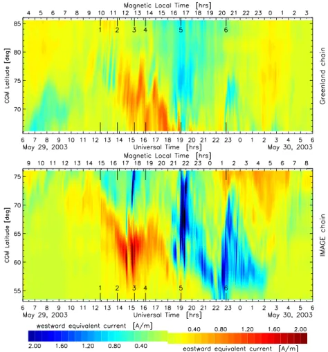
Fig. 9. East-west component of the equivalent ionospheric current derived from magnetometers measurements along the Greenland west

coast (top panel) and IMAGE (bottom panel) chains, respectively. Note that the chain meridians differ by about 5 hours in magnetic local time.

which is associated with the period of largest negative Bz (–32 nT), initiates the most active period, as seen by all in-dicators. It corresponds to the largest R-1 current and AE values. The largest ASY-H values (300 nT) are observed af-ter 19:06 UT and 22:30 UT. The SYM-H index reaches its largest negative value of –150 nT with about a 3–4 h delay at 23:15 and 02:00 UT. After the 22:50 UT substorm, the activ-ity decreases, with Bz alternating between positive and neg-ative values before turning positive and remaining so from 01:53 UT onward.

The AE and P CN magnetic indices are indicative of the large-scale, high-latitude current systems, namely the auro-ral electrojets and the trans-polar cap Hall current, which to-gether form the basis of the polar convection cells. We use these indices to guide our more detailed discussion of high-latitude current patterns inferred from two nearly-meridional magnetometer chains along the Greenland west coast and in Scandinavia (Fig. 9, upper and lower panels, respec-tively), the latter being known as IMAGE (Viljanen and H¨akkinen, 1997). The east-west oriented equivalent iono-spheric currents above Greenland were computed using the

inversion method proposed by Popov et al. (2001) and above Scandinavia using a method of upward continuation (e.g. Mersmann et al., 1979; Untiedt and Baumjohann, 1993).

In the following we use the term “Hall current” when refer-ring to these currents, although this is not exactly correct un-der all ionospheric conditions. FAC, electric field and iono-spheric conductance patterns can exist in a way such that the equivalent current (the divergence-free part of the horizontal ionospheric current) differs substantially from the Hall cur-rent (the cross-electric field curcur-rent). This case occurs specif-ically at electric conductance gradients, e.g., at the day/night terminator and at the edge of ionospheric plasma structures (see Sects. 2.4.2 and 2.4.3 in Untiedt and Baumjohann, 1993, for sample cases). At worst, both direction and intensity of the equivalent ionospheric current may have little in common with the true ionospheric current. Equivalent current pat-terns can therefore only be interpreted in a meaningful way if combined with other sources of information, e.g., magnetic indices (most of which are non-local measures) or current distributions derived simultaneously from different locations and from satellites. In spite of their limitations the large

(12)

C. Hanuise et al.: Impact of the 27–28 May 2003 solar events 139 spatial coverage and high time resolution of magnetometer

arrays make the equivalent currents a useful tool for study-ing ionospheric variations.

Both the P CN (Fig. 8) and the AE (Fig. 6) indices are rather small during the morning hours of 29 May 2003. Right after 12:25 UT, upon the arrival of the first shock, they in-crease modestly but sharply, indicating an enhancement of the auroral electrojet intensity and the trans-polar cap cur-rent. The rise is particularly clear in the Scandinavian sector (at that time located in the early afternoon sector) where it is accompanied by an equatorward motion of the equivalent current system which continues for several hours (Fig. 9). In contrast, it is noticed in the Greenland sector (located in the late morning) as only a short-lived spike followed by sev-eral small poleward propagating perturbations up to about 15:00 UT. In accordance with the increasing IMF By compo-nent after 14:00 UT an eastward directed DPY current sys-tem (Wilhjelm et al., 1978) develops in the noon sector above Greenland. The IMAGE chain witnesses the intensification and equatorward expansion of the eastward electrojet in the afternoon and evening sectors. Three peaks in the AE index, shortly after 13:30 UT, just before 15:00 UT and right af-ter 16:00 UT, are more or less clearly seen as enhancements of the current above Scandinavia but not in the Greenland sector. This is most likely due to the fact that Scandinavia is favourably placed under the eastward electrojet while Green-land is in the noon sector where the east-west current is weak (except for the DPY current). The 15:00 UT peak coincides with a rise of the P CN index, indicating that the Hall current intensity of the polar convection cells has increased.

A more pronounced increase of both the PCN and AE in-dices, however, appears at 19:00 UT and is most likely re-lated to the arrival of the most prominent solar wind shock which was discussed above. The eastward electrojet is driven further equatorward, and both Scandinavia and Greenland are exposed to relatively strong westward currents covering a wide range of latitudes. Greenland is located in the dusk and IMAGE in the pre-midnight sector. This observation sug-gests that the polar cap has expanded significantly, and the current observed above Greenland is part of the trans-polar cap Hall current while the very intense westward current over Scandinavia maps to the edge of the morning convection cell. This indicates that the shock caused a substantial change in the polar cap convection.

During the following hours the high-latitude current inten-sity diminishes while the westward current over Scandinavia is observed to move equatorward. Around 22:30 UT, upon the arrival of the last pressure pulse, the P CN and AE in-dices start to grow to high values and the westward electrojet intensifies again, accompanied by a poleward expansion (i.e. oval widening), first in the Scandinavian sector and shortly after above Greenland. The P CN and AE reach their peaks at about 23:00 UT (coinciding with the peak current densities measured by the two chains) and then decrease significantly to only moderate values. We can assume that both chains are located under the morning cell and observe that the con-vection intensifies greatly but does not move equatorward,

i.e. the expansion of the polar cap is only moderate. Only from about 23:30 UT onward is a weakening of the currents and a concentration of the westward current at lower latitudes (55◦–60◦CGM) observed while the higher latitudes (above 70◦CGM) are dominated by a moderately strong eastward current. It does not last long and is not particularly intense, probably because of reduced magnetic field merging between the interplanetary space and the magnetosphere (IMF Bz has become strongly positive). After 04:00 UT the storm seems to cease, and the polar cap current and electrojet intensity (as manifested by the PCN and AE indices, respectively) be-come very low. Both the Greenland and the IMAGE chain confirm this observation.

Finally, it is worth noting that all indicators agree to ev-idence a very large expansion of the auroral oval to lower latitudes. Quantitative indications come from the motion of the auroral electrojets and from the R-1 currents (see Sect. 4.2). Both suggest a 10◦ equatorward expansion of the auroral zone between 10:00 and 24:00 UT which pro-ceeds in steps, with intermittent relaxation and expansion. At least three major expansion periods are observed, the first from 12:30 UT to about 19:00 UT, the second from about 20:00 UT to 22:30 UT and the third from 23:30 UT to about 02:00 UT. The observation of aurora until 01:50 UT on 30 May at medium latitudes provides another observational evidence of such an expansion.

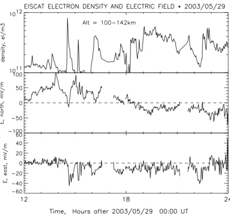
Figure 10 displays the electron density in the E-region and the electric field measured by EISCAT at Tromsø (66.6 mag-netic latitude) on 29 May between 12:00 and 24:00 UT. Dur-ing that period, EISCAT moves across the nightside of the Earth from 17:00 to 05:00 MLT in the morning, crossing the Harang discontinuity around 18:00 UT, as indicated by the reversal of the meridional component of the electric field. The electron density remains high, particularly during the main phase of the storm after 19:00 UT, due to electron pre-cipitation. When located under the eastward electrojet, EIS-CAT observes large northward electric fields with values up to 100 mV/m (equivalent to a westward plasma convection velocity of 2 km/s), which are well correlated with the cur-rent intensifications at the same latitude deduced from IM-AGE (Fig. 8). Large peaks in electron density indicate keV electron precipitation related to the substorm activity and au-roral intensifications or possibly to the events of magneto-spheric compression. Periods of large eastward electric field (northward convection velocity) occur which indicate either the propagation of convection vortices or northward motions of auroral arcs related to substorms. They are systematically associated with sharp enhancements in the E-region electron density, probably due to bursts of electron precipitation.

6 Thermosphere – ionosphere response

The reaction of the coupled ionosphere-thermosphere system to the magnetospheric energy input proceeds in several ways. Joule heating, due to the increased convection electric field and horizontal currents, is the primary auroral energy input

(13)

Fig. 10. Electron density in the ionospheric E-region and electric field on 29 May 2003 inferred from EISCAT measurements.

to the thermosphere besides particle precipitation. Knipp et al. (2005) have quantified the contribution of auroral energy to the total global heating budget of the upper atmosphere. While it usually amounts to about 17%, it may occasion-ally rise to 50% during intense geomagnetic storms, lead-ing to major perturbations of the thermosphere-ionosphere on a global scale. The role of solar wind pressure variations in heating the auroral ionosphere has also been discussed recently on the basis of MHD-simulations by Palmroth et al. (2004).

Indeed, at the latitude of the expanded auroral oval, Joule and auroral particle heating drive a divergent wind that forces upwelling of the neutral gas to a higher altitude resulting in neutral composition disturbance zones. Neutral winds, resulting from both the background daily circulation and perturbations induced by ion drag, transport auroral distur-bances away from their source regions towards middle and low latitudes (e.g. Burns et al., 1995; Fuller-Rowell et al., 1997). Such disturbances increase the proportion of molec-ular species in the upper atmosphere and this enhances ion-isation loss by dissociative recombination, resulting in a de-crease of ionization, the so-called negative storm phase (e.g. Pr¨olss et al., 1991; F¨orster and Jakowski, 2000). At auroral latitudes, the response of the ionosphere is, however, more complex: particle precipitations result in local increases of electron density, mainly at E-region altitudes (e.g. in Fig. 10) while convection flows transport F-region ionisation far from its source region. After this initial period, a decrease in

elec-tron densities in response to changes in the atmospheric com-position may be observed.

The increase of the thermospheric meridional circulation at auroral latitudes and the resulting density perturbations at middle latitudes have been observed and are presented in Sect. 6.1, while the more complex ionospheric signature at latitudes above 50◦_{are investigated in Sect. 6.2.}

6.1 Thermospheric wind and density

EISCAT measurements have been used to derive the merid-ional component of the thermospheric neutral wind from 27– 31 May at 250-km altitude (Fig. 11). Assuming no signif-icant vertical wind, the meridional wind component is de-rived from ion velocity measurements along the magnetic field line. This method has been extensively used to describe the thermospheric meridional wind at middle and high lat-itude during quiet magnetic periods (i.e. Buonsanto et al., 1999; Witasse et al., 1998). During disturbed periods at au-roral latitudes, vertical winds develop mainly at small spatial and temporal scales. The above method, however, allows one to derive reliable estimates of the large-scale daily vari-ation of the meridional wind. We have used here a 2-h run-ning average of the 1-min EISCAT data. As compared to the quiet time model (Witasse et al., 1998), Fig. 11 shows that the thermosphere circulation is already disturbed on 28 May in response to the PCIR observed at ACE (see Sect. 3 and Fig. 5). During daytime, the poleward wind is enhanced, while during nighttime an equatorward increase is observed

(14)

C. Hanuise et al.: Impact of the 27–28 May 2003 solar events 141 00 00 00 00 00 00 −600 −400 −200 0 200 400 600 Meridional wind m/s

May 27 May 28 May 29 May 30 May 31

Fig. 11. Meridional wind at 250-km altitude deduced from EISCAT observations from 27–31 May (red) in comparison with the quiet-time

model of Witasse et al. (1998) for summer conditions. High (low) solar activity is plotted as a dashed (solid) black line.

147 147.5 148 148.5 149 149.5 150 150.5 151 0 1 2 3 Density ratio 147 147.5 148 148.5 149 149.5 150 150.5 151−150 −100 −50 0 Dst Index

27 May 28 May 29 May 30 May

Atmospheric Density from CHAMP/ STAR Accelerometer

Fig. 12. Thermospheric density ratio deduced from the STAR accelerometer on board the CHAMP satellite. Red (green) symbols correspond

to a normalisation with the MSIS-90 (NRLMSISE-00) models run for quiet magnetic conditions. The blue line shows the Dstmagnetic index.

that maximizes during the 29–30 May night. The following night, the auroral thermospheric circulation has returned to normal, i.e. an equatorward wind at midnight with its ampli-tude twice as small.

The total thermosphere density is retrieved from STAR ac-celerometer measurements on board the CHAMP satellite at an altitude around 400 km. The method for obtaining the neutral density from the tangential acceleration is described in Bruinsma et al. (2004). Upper atmosphere winds are not

taken into account while retrieving the density. Resulting errors on densities maximize at 5% per 100 m/s wind am-plitude. Because the winds increase significantly at auroral latitudes during storms, the high latitude parts of the orbits are not used. The response of the thermosphere density is described in terms of its relative variations, normalized us-ing the semiempirical model MSIS-90 (Hedin, 1991) and the more recent one, NRLMSISE-00 (Picone et al., 2002). Both depend on the solar radio flux (given by the F10.7 index) and

(15)

Terminator

Night Day

(a) Fig. 13. (a) Two-hourly polar TEC maps showing TEC down to 50◦N latitude on 29 May 2003.

the magnetic activity (given by Ap indices), but quiet geo-magnetic conditions (daily Ap of 4) have been used here. These relative densities have been averaged over latitudes from –50◦to +50◦for every daytime orbit, from 27–30 May. Figure 12 shows the variation with time of the so-obtained daytime average relative density. It indicates that upon the arrival of the first interplanetary shock which marks the be-gin of the high activity period (12:30 UT on 29 May) the mid- and low-latitude density perturbation starts to grow and the density ratio increases from its 1.0–1.3 pre-storm num-bers to a peak of nearly 2.0 which is reached in the morning of 30 May, at the same time when Dst reaches a minimum.

6.2 Total electron content (TEC)

The integral of the electron density (called total electron content or TEC) along the ray path, from a GNSS satel-lite to a ground-based receiver, can be computed from

dual-frequency GPS measurements using the dispersive properties of the ionospheric plasma. After calibration (Sard´on et al., 1994) the measured slant TEC is mapped to the vertical by using a single layer approximation at an altitude of 400 km for the ionosphere. The computed TEC data are combined with the empirical TEC models, in order to generate TEC maps, (Jakowski, 1996) as shown in Figs. 13a–b.

Early on 29 May at 08:00 UT, the geomagnetic activity is low and the TEC exhibits a normal day-night structure (Fig. 13). The ionospheric convection increases afterwards, starting from the late afternoon/evening sector and moving the plasma towards the nightside across the polar cap. The strongest convection pattern develops around 20:00 UT, con-sistent with the PCN index increase shown on Fig. 8. This strong ionization enhancement is followed by a decrease in ionization. This negative storm phase, which starts in the re-gion of the geomagnetic pole around 22:00 UT, subsequently extends over the Northern Hemisphere and lasts during the

(16)

Terminator

Night Day

(b) Fig. 13. (b) Same on 30 May 2003.

full day on 30 May (Fig. 13b). It is rather surprising that the beginning of the negative phase does not occur in the auroral region, where the first impact of upwelling from the lower atmosphere is expected to appear. It might be that some transport effects also contribute in addition to thermospheric heating, but more knowledge of the local ionosphere would be needed in order to answer this question.

The temporal TEC variation at three selected latitudes along the 75◦_{W meridian (Fig. 14) shows a nearly}

simulta-neous and noticeable jump in the TEC by about 5×1016m−2 at 20:00 UT, just after the start of the most active phase of the storm. A second peak occurs at 23:00 UT at the auro-ral latitudes 70◦ and 60◦, associated with the second most active phase of the storm (see, for instance, the AE index, Fig. 6). During this period, the density variations are driven by precipitation and plasma transport. Keeping in mind the EISCAT observations (Sect. 5.2), this suggests that the main contribution to the TEC is provided by the E-region.

Im-mediately afterwards, the onset of the negative storm phase due to atmospheric composition changes is observed. At all latitudes, a sharp TEC increase is observed just after 06:00 UT, which may be attributed to the passage of the meridian in the midnight MLT sector where plasma may be transported from the dayside. The negative phase dominates at all latitudes after 08:00 UT on 30 May.

7 Space weather impacts

Numerous adverse effects result from the perturbations of the magnetosphere-ionosphere-atmosphere system. A few of them are discussed below. High energy auroral precipi-tation is the source of low altitude ionisation, leading to HF absorption (Sect. 7.1), and plasma instabilities, leading to scintillations (Sect. 7.2). Increased atmospheric density re-sults in satellite orbit perturbations (Sect. 7.3).

(17)

Fig. 14. Diurnal variation of TEC (red) for the latitudes 80, 70 and

60◦N along the 75◦W meridian on 29–30 May 2003. The monthly median TEC values (blue) are shown for comparison, together with the 3-hourly AP magnetic index (black).

7.1 HF absorption

D-region electron density is mostly controlled by hard X-rays, Lyman-α ionization of NO and, during solar events, electron precipitations at energies up to a few 100 KeV. In-creased D-region plasma density leads to inIn-creased absorp-tion of the cosmic radio noise in the 20–50 MHz range as measured by riometers. Figure 15a shows the data from 2 sta-tions of the Finnish chain (e.g. Ranta et al., 1981) on 29– 30 May. The effects of hard X-rays emitted by the flares on 27–28 May, and coincident with them, are not shown. A

so-Fig. 15. (a) Radio absorption around 30 MHz observed at 2 stations

of the Scandinavian riometer chain on 29 May 2003. Absorption peaks are seen simultaneously with the sudden commencements, especially at 12:25 UT and 19:06 UT. (b) Number of SuperDARN data points available from the Northern Hemisphere radar network. As a consequence of the radio blackout, it remains below 300 for the whole period and is close to zero from 09:00 UT until 18:00 UT (around 600 is typical under average conditions).

lar proton event started at 23:35 UT on 28 May and reached its maximum at 15:30 UT on 29 May. It produced an in-crease in the background absorption. In addition, peaks in absorption occur simultaneously with the sudden impulses. At 12:25 UT a peak is seen in the Abisko data but not at Ivalo, located at the same latitude, probably because of its later local time. At 19:06 UT peaks are present at both sta-tions (larger at Abisko). The peaks present at both stasta-tions at 14:30 UT (larger at Ivalo) is not related to any of the events listed in Table 3 but corresponds to a peak in EISCAT elec-tron density data in Fig. 10. All of these peaks in absorp-tion are probably associated with short-lived increases in D-region ionization, due to bursts of relativistic electron precip-itations generated by acceleration processes on auroral field lines.

The increase in radio absorption is at the origin of a ra-dio blackout and has a strong impact on HF radar obser-vations. Figure 15b shows the total number of data points available from the northern SuperDARN chain for deriving polar cap potential maps during the 24 h, starting on 29 May at 06:00 UT. This number remains always below 300 and is close to zero from 09:00 UT to 18:00 UT, as compared to an average number of at least 600 during usual conditions. This explains why it becomes impossible to derive representative potential maps and cross-polar potential values.

(18)

Fig. 16. Global maps of scintillation level estimated from high frequency GPS radio signal phase fluctuations on 29 May 2003. Each point

corresponds to a satellite-ground receiver link mapped to the sub-ionospheric point. Scale level: 0–0.25 for low, 0.25–0.5 for moderate, 0.5–0.75 for strong, >0.75 for severe. The successive maps show the equatorward expansion of the auroral zone and the increase in scintillation level associated with the storm.

While the radar echoes disappear at a global scale due to increased absorption, it is also well known that the arrival of a pressure perturbation at the magnetosphere leads locally to the creation of field-aligned currents and to the formation of characteristic vortex-like structures in the ionosphere (Araki, 1994). Radar echoes, produced by unstable density gradi-ents, resulting from increased precipitation (e.g. Zhou and Tsurutani, 1999), are locally triggered by a pressure pulse (Ballatore et al., 2001; Coco et al., 2005). This phenomenon is at the origin of the two increases in data point number seen in Fig. 15, one from 12:00 UT until 14:00 UT and the other one after 19:00 UT. Both of them begin at the time of the sudden commencements. Looking at the detailed Su-perDARN data, the echoes are returned from localized spots, slightly north of Tromsø at 12:00 UT and over Alaska around 19:00 UT.

7.2 Ionospheric scintillations

The high-latitude ionospheric plasma is structured at var-ious scales under the effect of plasma instabilities acting on electron density gradients related to electron precipita-tions. Scintillations are the fluctuations observed on radio signals as they are scattered in the forward direction by the F-region plasma fluctuations within the hundred of meters wavelength. They are a major source of disturbance for ground-satellites radio links. In the scope of the ESA Space Weather Pilot Project, CLS (Collecte Localisation Satellites) has developed a prototype service to monitor ionospheric

scintillations at a global scale in near real time. An empir-ical index is derived from the analysis of GPS signal pertur-bations provided by the IGS worldwide permanent network of about 300 receivers. It is derived from the high-frequency fluctuation of the GPS dual frequency phase difference that only contains the effect of ionospheric refraction on the sig-nals. This index is scaled by comparison with scintillation monitor records from Douala (Cameroon).

The algorithms have been applied to the 29–30 May period for 6-h time intervals and the result is presented in Fig. 16. Each point on the map corresponds to an individual measure-ment with a 30-s resolution. Starting from a relatively quiet scintillation level before 12:00 UT on 29 May (Fig. 16a), the beginning of the storm at 12:25 UT triggers both an increase in the scintillation level and an equatorward expansion of the scintillation region identified to the auroral zone (Fig. 16b). These effects maximize during the 18:00–24:00 UT period (Fig. 16c) already identified as the period of maximum ex-pansion of the auroral zone from the magnetometer and au-roral data. The ionosphere returns slowly to a quiet level at the end of the storm (Fig. 16d). These maps have to be in-terpreted with care. For example, the number of available ground stations influences their appearance, as is the case over North America. In this region, the scintillations look more intense only because the number of points is larger. Similarly, a region of high scintillation level appears over the Mediterranean Sea between 18:00 UT and 24:00 UT. It is as-sociated with signals received by at least 3 stations in Spain and 2 stations in Italy, and is probably due to spurious effects.

(19)

Fig. 17. Time variation of the scintillation index derived from 30-s

samples at three high-latitude stations and one sub-auroral station from 29 May at 06:00 UT to 30 May at 06:00 UT. Different colours correspond to different GPS satellites. The variations in scintillation level follow the variations in the storm intensity, as shown by the magnetic indices, especially at Kiruna. Also note the delay from the auroral zone to lower latitudes due to propagation of storm-induced perturbations.

Nevertheless, its origin is not yet understood and further in-vestigation is needed.

The time variations of the scintillations index have been plotted at three auroral stations located at Kiruna, Churchill and Fairbanks (respective magnetic latitudes 65◦N, 69◦N and 51◦N) and one sub-auroral location (Metsahovi, mag-netic latitude 57◦N), for a 24-h interval starting on 29 May at 06:00 UT (Fig. 17). Each colour corresponds to one GPS satellite. During quiet periods, the scintillation level is con-trolled by the motion of the station into and out of the auro-ral zone. The main effects of the storm are the enlargement of the auroral oval through the increased convection elec-tric field and solar wind pressure and the enhancement of the ionosperic scintillation level through intensified particle precipitation and increasingly effective plasma instabilities. The relation with the storm intensity is particularly clear in the Kiruna data, if one considers the global envelope of all the individual signals. Its variations are quite similar to the variations of the indices described previously, especially to those of the AE index (Fig. 6, centre panel). The start of the

storm is also very clear at Churchill and later variations of the scintillation index are broadly similar to those observed at Kiruna. This is no longer true at Fairbanks, where the storm started during the night. The difference between UT and LT is such that specific signatures of the storm are difficult to be isolated apart from a general increase in scintillation level. In the European longitude sector, the peaks in scintillation index are also clearly present at sub-auroral latitudes, as seen in Metsahovi, Finland. Compared to the Kiruna observations, their level is weaker and their appearance is delayed, as ex-pected from the propagation of storm-induced perturbations from the auroral zone to lower latitudes. At 05:00 UT on 30 May, the ionosphere has returned quiet everywhere. 7.3 Satellite drag

As described in Sects. 6 and 6.1, geomagnetic storms re-sult in heating and upwelling of the thermosphere, which means an increase in the atmospheric density at a given al-titude and therefore an increase in the drag force exerted on Low Earth Orbit (LEO) satellites. Because empirical ther-mosphere models fail to reproduce correctly the magnitude of the perturbation (e.g. Emery et al., 1999; Lathuill`ere and Menvielle, 2004), the impact on the positioning is evidenced on the estimated drag coefficients in the orbit restitution pro-cess and on the orbit position error in orbit prediction.

The SPOT-2, SPOT-4, SPOT-5 and ENVISAT satellites have an on-board DORIS range measurement instrument whose aim is the precise satellite orbit determination (Tav-ernier et al., 2003). Everyday, operational 24-h precise or-bits are calculated by the French Space Agency using a min-imization scheme of the error between calculated and mea-sured satellite-ground station radial velocity measurements. These orbit restitutions need precise acceleration models, as DORIS satellites orbit at an altitude around 800 km, where the drag effects cannot be neglected due to the important cross-sectional surface of the platforms. The mathematical model of the orbit trajectory uses, for drag estimation, the DTM94 empirical neutral model (Barlier et al., 1978; Berger et al., 1998). It directly depends on physical parameters, and in particular, the F10.7 solar flux and the Kp geomagnetic indices. Minimization is obtained by applying different co-efficients, among them the drag coefficient which has to be applied to the density model, and which is estimated every 6 h.

The top panel of Fig. 18 displays the estimations of the air drag coefficient between 27 May and 1 June. The value of this coefficient would be 1.0 if the model was perfect. During most of the period, the estimations present a small variation between 0.7 and 1.3. During the 29 May storm, extreme val-ues ranging from 0.4 to 2.2 are obtained, indicating the inad-equacy of the empirical model. The bottom panel of Fig. 18 shows the differences in the along-track satellite position be-tween the 1-day extrapolated and the 1-day adjusted orbits. On 29 May this difference reaches about 60 m on SPOT 5 and ENVISAT, compared to the usual mean values of the order of 10 m.

(20)

27-May 28-May 29-May 30-May 31-May 01-Jun

0 10 20 30 40 50 60 70 RMS (m) SPOT2 SPOT4 SPOT5 ENVISAT

27-May 28-May 29-May 30-May 31-May 01-Jun

0 1 2 Drag coefficient SPOT2 SPOT4 SPOT5 ENVISAT

Fig. 18. Top panel: variation of the 6-h air drag coefficient estimated from data taken by the DORIS instrument flown on the ENVISAT and

SPOT satellites using the DTM model. In the vicinity of the storm, the drag parameters are perturbed and their values range between 0.5 and 2.2 compared to the nominal value of 1. Bottom panel: along-track mean position differences using 1-day extrapolated and 1-day adjusted orbits.

Table 4. May and October 2003 geospace storm main parameters.

Storms /2003 May 29 October 29 October 31 November 20

Storm intensity:

Minimum Dst (nT) -130 -363 -401 -472

Magnetic cloud at ACE |B| (nT) observed |B| (nT) –Gonzalez et al. 35 34 50 93 40 69 56 33 Initial CME velocity (km/s)

ACE SW velocity (km/s) Estimated delay (hours)

1370 750 36 1785 2000 19 1948 1500 19 1660 730 46 Maximum AE (nT) 2500 3500 3000 2500 Maximum Kp / am (nT) 9- / 388 90 / 551 90 / 592 90 / 499

Table 4: May and October 2003 geospace storm main parameters

8 Discussion and conclusion

One of the objectives of a comprehensive analysis of solar-terrestrial disturbances during specific events is to deter-mine, from one event to the other, the most pertinent fac-tors which drive the various responses to the solar energy inputs. We have therefore chosen to compare the 29 May magnetic storm with the three major storms of the strongly disturbed October–November 2003 period (the Halloween storms of 29–31 October and the 20 November storm, Gopal-swamy et al., 2005a and reference therein). Table 4 shows the main parameters of these events. When measured by the

Dstmagnetic index, the May storm appears less intense than

the October–November storms. According to the classifica-tion of Gonzalez et al. (1994), the 29 May storm belongs to the “intense storm” category (minimum Dst=–131 nT) while

the Halloween storm is a more severe one and falls into the

superstorm category (minimum Dst=–401 nT). It is now well

known (Gosling, 1993) that the central role in the chain of events leading to major geospace disturbances is attributed to CMEs through the association of their strongly southward magnetic field with the increased solar wind pressure. As already observed (Gosling, 1993) the flare intensity (as de-fined by the X-ray flux observed by GOES) does not corre-late to the storm intensity (as defined by the Dst). Although

the 20 November storm is the largest one of solar cycle 23, its source CME is associated with an M-class flare while the 29 May storm follows a stronger X-class flare. More sur-prisingly, the halo CME generated by the flare of 4 Novem-ber, estimated to have reached a maximum between X28 and X45 (Woods et al., 2004; Thomson et al., 2004; Brodrick et al., 2005), did not create any significant magnetospheric effect. An important characteristic of the October storms is that they were triggered by ultra fast CMEs which resulted