Crystallographically Consistent Percolation Theory
for Grain Boundary Networks
by Megan E. Frary
B. S., Materials Science and Engineering Northwestern University, 1999 M. S., Materials Science and Engineering
Northwestern University, 2001
SUBMITTED TO THE DEPARTMENT OF MATERIALS SCIENCE AND ENGINEERING IN PARTIAL FULFILLMENT OF THE REQUIREMENTS FOR THE DEGREE OF
DOCTOR OF PHILOSOPHY IN MATERIALS SCIENCE AND ENGINEERING AT T-IF.
MASSACHUSETTS INSTITUTE OF TECHNOLOGY
JUNE 2005
MASSACHUSE
OF TECH:
JUL 2 i
© 2005 Massachusetts Institute of Technology. All rights reserved.
Signature of Author:
Certified by:
Accepted by
.
x" Departmen6f Materials Science and Engineering May 16, 2005Christopher A. Schuh Danae and Vasilios Salapatas Assistant Professor of Metallurgy
Thesis Supervisor
Gerbrand Ceder Chair, Departmental Committee for Graduate Students
ARCH-IVts TS NSUmE IOLOGY RIES2005 RIES LIBRAM I
Crystallographically Consistent Percolation Theory
for Grain Boundary Networks
by Megan E. Frary
Submitted to the Department of Materials Science and Engineering on May 16, 2005 in Partial Fulfillment of the Requirements for the Degree of
Doctor of Philosophy in Materials Science and Engineering
ABSTRACT
Grain boundaries are known to play a role in many important material properties including creep resistance, ductility and cracking resistance. Although the structure and properties of individual boundaries are important, the overall behavior of the material is determined largely by the connectivity of grain boundaries in the microstructure. Grain boundary networks may be studied in the framework of percolation theory by classifying boundaries as special or general to the property of interest. In standard percolation theory, boundaries are randomly assigned as special or general; however, this approach is invalid in realistic grain boundary networks due to the requirement for crystallographic consistency around any closed circuit in the microstructure. The goal of this work is to understand the effects of these local constraints on the connectivity and percolation behavior of crystallographically consistent grain boundary networks. Using computer simulations and analytical models, the behavior of crystallographically consistent networks is compared to that of randomly-assembled networks at several different length scales. At the most local level, triple junctions and quadruple nodes are found to be preferentially coordinated by special and general boundaries, leading to nonrandom network topologies that are quantified using topological parameters. Although the properties of the simulated microstructures, including connectivity length and average cluster radius of gyration, are described by the same scaling exponents as in standard percolation theory, the amplitude prel'actors in the scaling relationships are changed as a result of the crystallographic constraint. The percolation threshold, an important parameter in microstructural design, is also found to differ from that of standard percolation theory by as much as 0.05. Although all of the simulated grain boundary networks studied here are distinctly nonrandom, no two cases have the same behavior, the details of which depend strongly on the specific microstructural model. Therefore, a unified approach for locally correlated percolation problems is developed that allows the effects of the requirement for crystallographic consistency to be compared directly from system to system. This new approach can be extended beyond the study of grain boundary networks to include other locally-correlated percolation problems.
Thesis Supervisor: Christopher A. Schuh
Acknowledgements
I would like to acknowledge the members of my thesis committee, Professor Bernhardt Wuensch and Professor Linn Hobbs, for their time and insightful comments. Their suggestions lead me to consider some interesting problems that I would not have otherwise addressed. I also greatly appreciate the patience they had with the seemingly endless math that I presented.
I would also like to thank the other students in our group, Yuttanant (Vee) Boonyongmaneerat, Andy Detor, Corinne Packard, Ying Chen, Jason Trelewicz, and Jeff Zelinski, who made being at work as much as I was as enjoyable as possible.
Finally, I would like to thank my advisor Chris Schuh. When I was assigned as an undergraduate to work with Chris almost seven years ago, I could not possibly have imagined what would have happened since then. I owe much of who I am as a scientist to the enthusiastic and patient guidance of Chris. I am fortunate to have had an advisor who led by example, and who pushed me to work harder and tackle more challenging problems than I had thought possible. As I move on in my own career, I can only hope to make as much of a difference to one of my students as Chris has made to me.
Table of Contents
A b s t r a c t ... 3
A c k n o w le d g e m e n ts ... 5... 5
List of Figures ...ist of Figures...9
List of Tables...ist of Tables... 17
N o m e n c la turcla tu r e ... 1 9 1 . In tro d u c tio n . ... 2 3 1.1. The Role of Grain Boundaries in Material Properties ... ... 23
1.2. Local Connectivity of Grain Boundaries ... 25
1.3. Percolation-Based Models of Grain Boundary Networks ... ... 26
1.4. Correlations among Grain Boundaries at a Triple Junction ... ... 29
1.5. Influence of Crystallographic Constraint on Grain Boundary Connectivity ... 31
1.6. Problem Statement 33 2 . S im u la tio n P ro c e d u re s ... 3... 3 5 3 2.1. Assignment of Grain Structure ... ... 36
2.2. Assignment of Grain Orientations ... 38
2.3. Determination of Grain Boundary Character ... 41
2.4. Identification of Grain Boundary Clusters ... 46
:3. Crystallographic Constraint at Triple Junctions ... 49
3.1. Topology of Simulated Grain Boundary Networks ... 49
3.2. Analytical Model for the Triple Junction Distribution ... 54
3.2.1. Analytical Approach ... 54
3 .2 .2 . L o cal T ran sitio n P ro b ab ilities ... 55
3.3. C oncluding R em arks ... 59
4. Crystallographic Constraint at Quadruple Nodes ... . . 61
4.. 1. Q u a d ru p le N o d e D istrib u tio n s ... 61
4..2. Crystallographic Constraints around Quadruple Nodes ... 65
4.2.1. Relationship between Triple Junction and Quadruple Node Distributions 66 4.2.2. Configurational Entropy of Grain Boundary Networks ... 71
4 .3 . C o n c lu d in g R e m a rk s ... 7 3 5. Percolation and Scaling Behavior of Grain Boundary Networks ... 75
5.1. Percolation Thresholds for Grain Boundary Networks ... 76
5.1.1. Percolation Thresholds in Two-Dimensional Grain Boundary Networks 76 5.1.2. Percolation Thresholds in Three-Dimensional Grain Boundary Networks 78 5.2. Scaling Laws for Grain Boundary Networks in the Thermodynamic Limit ... 80
5.3. Medium-Range Effects of Crystallography ... 87
5.4. Effects of Lattice Topology and Dimensionality ... 95
5.5. A Critical Length Scale for Grain Boundary Networks ... 98
5.6. Concluding Remarks ... 99
6. A Unified Approach for Locally Correlated Percolation Problems . ... 101
6.1. Topological Descriptions of Locally-Correlated Systems ... 101
6.2. Determination of the Percolation Phase Boundary ... 110
6.3. Effects of Local Correlations on Connectivity Length ... 118
C o n c lu s io n s ... 1 2 3 Directions for Future W ork ... 125
R e f e r e n c e s ... 1 2 7 Appendix A: Derivation of the Deviation Limit Rule ... 135
Appendix B: Derivation of Local Transition Probabilities for Fiber Textured
Microstructures ... ... 141
Appendix C: Maximum Entropy Distribution ... 155 Appendix D: Topological Parameter Expressions for the Triple Junction Distribution ... 159
Appendix E: Correlations beyond the Nearest-Neighbor Level in Grain Boundary
Schematic representation of the propagation of an intergranular crack. Thin, solid lines are general boundaries, dashed lines are special boundaries, and the thick
line is the crack. At the triple junction with two special boundaries (labeled a and
b), crack propagation is arrested.
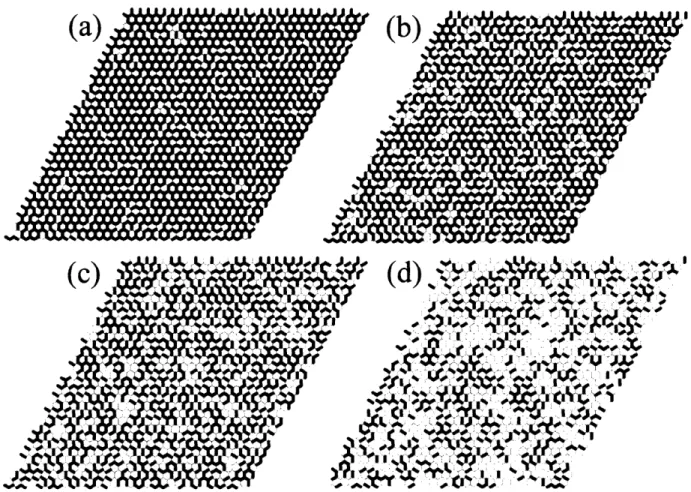
Simulated 2-D microstructures using a honeycomb grid on which grain boundaries (the edges of the hexagons) are randomly assigned as special (thin lines) or general (thicker lines) with probability p. The fraction of special boundaries is (a)p = 0.15, (b)p = 0.35, (c)p = 0.55 and (d)p = 0.75.
An idealized triple junction between three grains, A, B, and C. For a complete circuit around the junction (dashed line), three grain boundaries, a, b, and c, are crossed, giving three step-changes in Euler orientation space. Since the beginning and end of the circuit lie in the same grain, these changes must sum to zero; misorientation is conserved.
Triple junction distributions from existing experimental data (points), covering a range of materials and crystal systems, including pure metals, intermetallic alloys and superconducting oxides, with low-angle thresholds t between 4 and 15°.
These data are compared to the triple junction distribution for a random assemblage of boundaries as given by Eq. (1.5) (solid lines).
Procedure for assembling a crystallographically consistent grain boundary network.
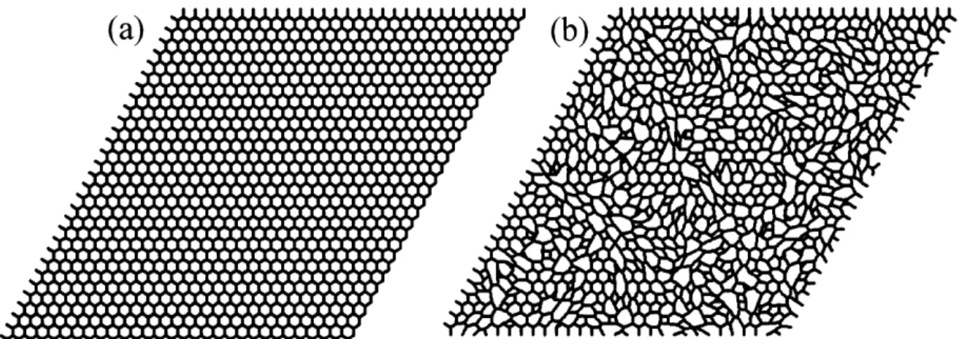
Examples of two-dimensional networks with 30 grains per side that have either (a) a honeycomb structure or (b) an irregular structure.
Schematic illustration of the procedure used to create irregular lattices. The four grains that are effected by the reorientation of the bold boundary are labeled A, B,
C, and D. The boundary to be reoriented (the bold line) has neighboring
boundaries labeled nl, n2, n3, and n4. When the boundary is reoriented (b), the number of sides in grains B and D decreases by one, while the number of sides in grains A and C increases by one.
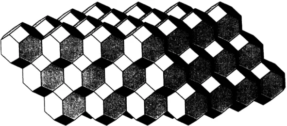
Schematic illustration of the three-dimensional grain structure used in the simulations where grains are modeled as 14-sided tetrakaidecahedra.
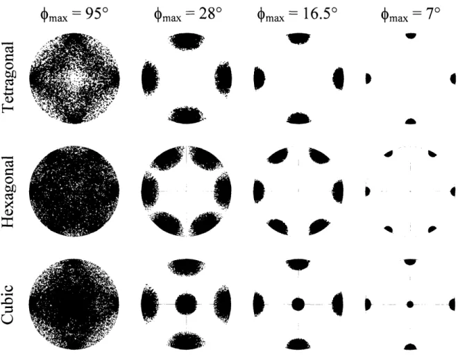
Pole figures for fiber textured polycrystals. Top row: (100) pole figures for tetragonal polycrystals, middle row: (1070) pole figures for hexagonal polycrystals, and bottom row: (100) pole figures for cubic polycrystals. The sharpness of the texture is increased (moving left to right) by decreasing the maximum rotation angle for any grain, (4max, as indicated above the different
columns.
Pole figures for general textured polycrystals. Top row: (100) pole figures for tetragonal polycrystals, middle row: (100) pole figures for hexagonal polycrystals, and bottom row: (100) pole figures for cubic polycrystals. The
List of Figures
Figure 1.1: Figure 1.2: Figure 1.3: Figure 1.4: Figure 2.1: Figure 2.2: Figure 2.3: Figure 2.4: Figure 2.5: Figure 2.6:Figure 2.7: Figure 2.8: Figure 2.9: Figure 2.10: Figure 2.11: Figure 2.12: Figure 2.13: Figure 2.14: Figure 3.1:
sharpness of the texture is increased (moving left to right) by decreasing the maximum rotation angle for any grain from 95° to 7°.
(001) pole figure illustrating the grain orientations that result from rotating a grain with an initial cube texture (open circles) through one of the four unique 3 rotations. The resulting orientation after each possible rotation is given by a different symbol (squares, circles, diamonds and triangles).
(001) pole figures for simulated twinned polycrystals with L = 100 (10,000 total grains). The number of twin rotations per grain, t, is indicated above each pole figure. Although the number of grain orientations mapped in each pole figure is constant, more of the grains assume unique orientations as t increases, resulting in more unique points appearing in the pole figure.
The disorientation angle distribution for fiber textured (a - c) and general textured (d - f) microstructures with either tetragonal (a, d), hexagonal (b, e) or cubic (c, f) symmetry. The different distributions correspond to different maximum rotation angles, max, as labeled on the graphs. For the general textured microstructures, the distribution of disorientation angles for a random assemblage of polycrystals with the given symmetry is also shown.
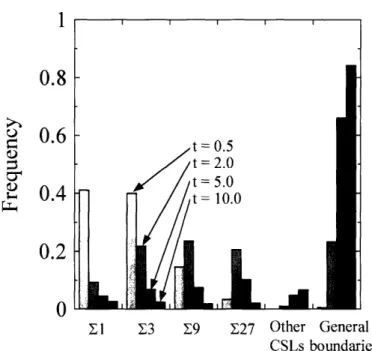
The frequency of twin variant boundaries (E3n), other CSL boundaries (with E < 29), and general boundaries is plotted for simulated microstructures with t = 0.5, 2.0, 5.0 or 10.0 twin rotations per grain.
Fraction of low-angle boundaries, p, as a function of the sharpness of texture, given by the rotational tolerance, qmax, for polycrystals with cubic, hexagonal, and tetragonal symmetry where the low-angle threshold is 15°. For the fiber textured microstructures, the curves are truncated at the minimum value of p achievable as explained in the text.
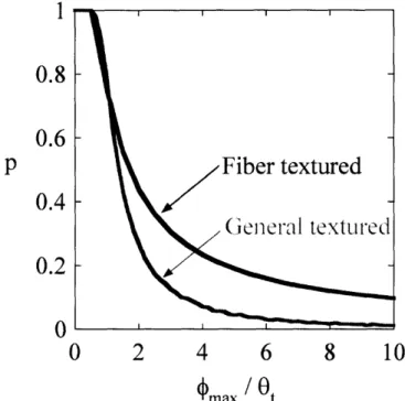
Fraction of low-angle boundaries, p, as a function of the rotational tolerance, max,
normalized by the low-angle boundary threshold, t for fiber textured or general textured polycrystals.
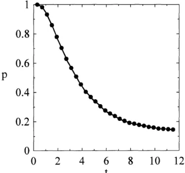
Fraction of special (CSL) boundaries, p, as a function of t, the number of twin rotations per grain for simulated cubic polycrystals.
The probability of a simulated fiber textured microstructure containing a percolating cluster of general boundaries as a function of p, the fraction of special boundaries in the microstructure. The width of the transition region, from percolating to non-percolating, decreases as L, the number of grains per side in the simulated structures, increases. The dotted lines indicate the error bar on the percolation threshold for simulations with L = 1000.
Complementary spatial distribution of general (left column) and special boundaries (right column) forp = 0.5 on small, two-dimensional honeycomb (a
-h) or irregular lattices (i, j). The polycrystals were assembled either randomly (a and b) or with crystallographic consistency (c, d: general textured; e, f: twinned, g - j: fiber textured).
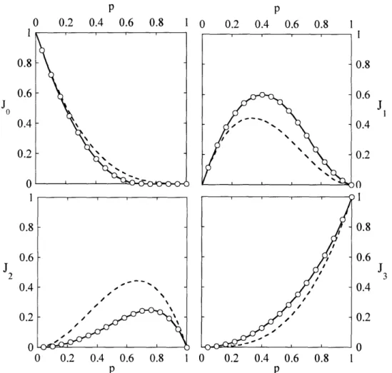
Triple junction distribution for simulated microstructures with crystallographic consistency (fiber texture: solid lines, general texture: dashed lines). Also shown are the TJD for a random network (dotted lines, Eq. (1.5)), and experimental triple junction distributions, where the symbols are the same as in Figure 1.4.
Local transition probabilities, HY , for (a) y = 0, (b) y = 1, and (c) y = 2, which give the local probability of assigning the next boundary as a special boundary. The expectation value for a random lattice is given by the dashed line, Hy = p. Deviations above this line indicate that a special boundary is more likely to coordinate the junction, while deviations below indicate that a general boundary is more likely.
Analytical triple junction distribution for fiber textured microstructure given by Eqs. (3.1) and (3.3) (solid line). Also shown are the simulated fiber textured microstructures (points) and the distribution for a random lattice as given by Eq.
(1.5) (dashed lines).
(a) The four tetrakaidecahedral grains that comprise a quadruple node. The grains are labeled Gi (i = to 3), and boundaries are labeled with lower-case letters. (b) The shared faces of the tetrakaidecahedra are the grain boundaries in the quadruple node. The lightly shaded boundaries have general character, while the darker boundaries are special. The six boundaries are labeled a through f (c) Two-dimensional topological map of the same quadruple node as in part (b) where thinner lines indicate general boundaries and thicker lines are special boundaries. The four grains, which have the same shading as in part (a), are the enclosed areas between the lines and grain G3 is the entire area outside the
triangle. The circuit in (c) represents a second-order constraint involving four grains and four boundaries.
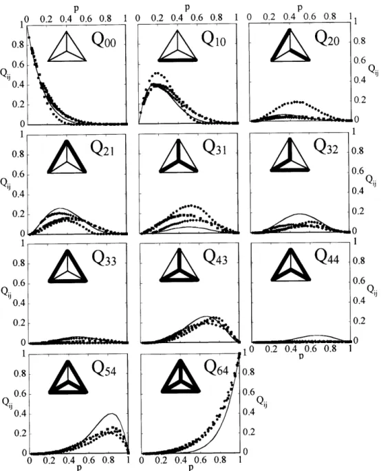
The quadruple node distributions for simulated three-dimensional fiber textured (circles), general textured (squares), and twinned (diamonds) microstructures. The lines represent the QND for the case where boundaries are randomly assigned character (Eq. (4.1)). The 2-D topological map is also shown for one configuration of each type of quadruple node, where thinner lines are general boundaries and thicker lines are special boundaries.
The topological map for a Q21 quadruple node, where the boundaries are labeled a through f with special boundaries indicated by the thick lines and general boundaries by thinner lines. Three of the triple junctions are labeled as i, ii and
iii, and are assigned a character in order to form this specific Q21 quadruple node. The possible assignments at each triple junction are shown in columns i, ii and iii on the right, where the correct assignment that leads to this specific quadruple node is indicated by the dashed box.
The error between Qij as predicted by Eq. (4.6) and as found from the simulations for (a) fiber textured, (b) general textured and (c) twinned microstructures. Positive AQij values indicate that Eq. (4.6) overpredicts Qij, while negative AQij values indicate underprediction of Qij. The maximum error for each microstructure is shown by the dashed lines and is -0.05 for each. However, the Figure 3.2: Figure 3.3: Figure 3.4: Figure 4.1: Figure 4.2: Figure 4.3: Figure 4.4:
Figure 4.5: Figure 5.1: Figure 5.2: Figure 5.3: Figure 5.4: Figure 5.5: Figure 5.6: Figure 5.7:
majority of the Qij are predicted quite accurately, and 75% of these errors lie within the dotted lines at AQij - 0.015.
The decrease in configurational entropy (Eq. (4.8)) from the maximum entropy configuration, S, for fiber textured (circles), general textured (squares) and twinned (diamonds) microstructures due to crystallographic constraints. For nearly every value of p in all three systems, the decrease in entropy is greater when both first- and second-order constraints are imposed (filled points) than with first-order constraints only (open points).
The complementary relationship between a percolating 1-D chain of special boundaries (darker shading) and a 2-D surface of general boundaries (lighter shading). The presence of the percolating chain of special boundaries removes the possibility of a sample-spanning surface of general boundaries, as at least one boundary on the surface of general boundaries must be part of the percolating cluster of special boundaries.
The average radius of gyration, Rs, as a function of cluster mass for simulated honeycomb lattices at the percolation threshold; for random networks p = 0.653 (diamonds), for general boundary networks p = 0.601 (squares, offset in Rs by a factor of 10), and for special boundary networks p = 0.689 (circles, offset in Rs by a factor of 100). The lines represent the best fit of Eq. (5.1).
The cluster mass distribution at the percolation threshold for random networks at
p = 0.653 (diamonds), general boundary networks atp = 0.601 (squares, offset in
ns by a factor of 10), and special boundary networks at p = 0.689 (circles, offset in ns by a factor of 100). The results were obtained from simulations on 2-D honeycomb lattices. The lines represent the best fit of Eq. (5.2).
The connectivity length 4 as a function of pv -pl both below (a) and above (b) the critical point (given in Table 5.1) for random networks (diamonds), general boundary networks (squares, offset in by a factor of 10), and special boundary networks (circles, offset in 4 by a factor of 100). Above the percolation threshold, the contribution of the lattice-spanning cluster is not included in the determination of 4. These simulations used 2-D honeycomb lattices, and the lines represent the best fit of Eq. (5.3).
The dependence of the strength of the "infinite" or lattice-spanning cluster, P, as a function of p - p,. The values of Pc are given in Table 5.1. The diamonds
represent random networks, the squares general boundary networks (offset in P by a factor of 3), and the circles special boundary networks (offset in P by a factor of 9). The results were obtained from simulations on 2-D honeycomb lattices. The lines represent the best fit of Eq. (5.4).
For 2-D honeycomb networks, the cluster mass distribution at the percolation threshold is plotted for small values of s in random networks at p = 0.653 (open diamonds) and special boundary networks atp = 0.689 (filled circles).
Taxonomy of grain boundary clusters. The left column illustrates clusters with different masses. In the middle column, some topologically unique animals with s = 9 are shown. The animals are labeled a-b-c, where a is the number of J1, b the
Figure 5.8: Figure 5.9: Figure 5.10: Figure 5.11: .Figure 5.12: Figure 5.13 Figure 5.14: Figure 6.1: Figure 6.2:
number of J2 and c the number of J3junctions in the animal. The right column shows some of the conformations available to the s = 9, 2-8-0 animal, each of which has a different radius of gyration.
The fraction of animals of mass s = 9 with each possible topology in (a) special boundary networks (FsB) and (b) random networks (FR). In (c), FsB is normalized by FR for the 8 topologically unique animals with s = 9 on a honeycomb lattice. A representative conformation is also shown for each animal in (c). These simulations were performed atp = 0.55.
The animal distribution, F, as a function of the number of J2 junctions needed to construct the animal in random networks (filled circles) and special boundary networks (open circles) for clusters with s = 29, 69, 109, 149, and 189. These simulations were performed atp = 0.55.
For 2-D honeycomb networks, average radius of gyration, R, is plotted for small values of s in random networks at p = 0.653 (open diamonds) and special boundary networks atp = 0.689 (filled circles).
For 2-D honeycomb networks, the cluster mass distribution is plotted for small values of s in random networks at p = 0.653 (open diamonds) and general boundary networks atp = 0.601 (filled squares).
The fraction of animals, FSB, with each possible topology in special boundary networks, normalized by the respective animal frequency in random networks, FR. These simulations were done at p = 0.55. The filled squares are for 2-D honeycomb lattices (where only eight animals are possible), and the solid line is an exponential fit to those data. The unfilled circles are for 2-D irregular lattices
in which 25% of the grains had six sides. In this case, more than 250 animals are possible.
For 2-D irregular networks, the cluster mass distribution is plotted for small values of s in: (a) special boundary networks at p = 0.689 and (b) general boundary networks at p = 0.601. The different points correspond to different fractions of grains with six sides.
For 3-D tetrakaidecahedral networks, the cluster mass distribution is plotted for small values of s in random networks withp = 0.220 (unfilled diamonds in (a) and (b)), special boundary networks at p = 0.280 (filled circles in (a)), and general boundary networks atp = 0.152 (filled squares in (b)).
Coordination tetrahedron whose vertices are the triple junction populations (i.e., Jo, J, J2 and J3). The trajectories show the evolution of the TJD through this
space for random networks (black curve), special boundary networks (green curves) or general boundary networks (red curves) from p = 0 (Jo vertex) to p = 1 (J3 vertex). (a) The black points represent the percolation thresholds determined in Chapter 5. (b) The relative position of the trajectories can be more easily observed in projection along the J3axis.
The triple junction distributions for experimental microstructures (blue points) are compared to the trajectory for a randomly assembled network (black curve) or
crystallographically consistent networks (green curves). In (a), the data points are the same data as presented in Figure 1.4, while the light green and dark green curves are for fiber textured and general textured microstructures, respectively. In (b), the data points were gathered by Schuh et al. for microstructures where the boundaries were classified as CSL vs. non-CSL and the green curve is for the twinned microstructural family.
Schematic network structures corresponding to the segregated state (left, with 'iso > 0) along the Jo - J3 edge or ordered state (right, with riso < 0) along the J1 - J2
edge. The surface plotted in the coordination tetrahedron is for points with riso = 0 (Eq. (6.3)) and contains the trajectory for a randomly assembled network (black curve).
Schematic network structures corresponding to the elongated state (left, with CE
< 0) along the Jo - J2- J3 face or clumpy state (right, with riCE > 0) along the Jo
-JI - J3 face. The surface plotted in the coordination tetrahedron is for points with iCE = 0 (Eq. (6.4)) and contains the trajectory for a randomly assembled network (black curve).
Schematic representation of the four unique topological states defined by (i) qso >
O
and rCE > 0 (segregated and clumpy), (ii) rso > 0 and rICE < 0 (segregated and elongated), (iii) riso < 0 and riCE > 0 (ordered and clumpy), and (iv) riso < 0 andriCE < 0 (ordered and elongated). At the Jo and J3 vertices, all four states
converge.
For the three microstructural models studied here, the evolution of the grain boundary networks is plotted as a function of the topological parameters (CE and riso) and p, the fraction of relevant boundaries (special boundaries for the green curves and general boundaries for the red curves). The black curve is for randomly assembled networks. (a) The black points represent the percolation thresholds determined in Chapter 5. (b) The relative position of the trajectories can be more easily observed in projection along the p-axis where each of the four quadrants represents one of the four topological states. In (b), the intial location of the trajectory in the p = 0 plane is indicated by a circle.
In the coordination tetrahedron, the points where (a) less than 50% of the simulated networks contained a percolating cluster, (b) greater than 50% contained a percolating cluster, and (c) between 25 and 75% contained a percolating cluster. The data points in (c) are used to determine the polynomial fit for the percolation surface (Eq. (6.7)), also shown in (c).
In terms of the topological parameters, the points where (a) less than 50% of the simulated networks contained a percolating cluster, (b) greater than 50% contained a percolating cluster, and (c) between 25 and 75% contained a percolating cluster. The data points in (c) are used to determine the polynomial fit for the percolation surface (Eq. (6.8)), also shown in (c).
For (a) randomly assembled, (b) fiber textured, (c) general textured and (d) twinned microstructures, the known trajectories are plotted for special boundary clusters (green curve changing to blue) and general boundary clusters (red curve Figure 6.3: Figure 6.4: Figure 6.5: Figure 6.6: Figure 6.7: Figure 6.8: Figure 6.9:
Figure 6.10: Figure 6.11: Figure 6.12: .Figure B. 1: Figure B.2: Figure B.3: Figure B.4: Figure B.5:
changing to blue). The non-percolating part of the random network trajectory is shown in black as it applies to either special or general boundaries. The color change corresponds to the real percolation threshold (Table 5.1) and should occur when the trajectory intersects the surface defined by Eq. (6.7). The errors between the real and predicted values are summarized in Table 6.1.
For (a) randomly assembled, (b) fiber textured, (c) general textured and (d) twinned microstructures, the known trajectories are plotted for special boundary clusters (green curve changing to blue) and general boundary clusters (red curve changing to blue). The non-percolating part of the random network trajectory is shown in black as it applies to either special or general boundaries. The color change corresponds to the real percolation threshold and should occur when the trajectory intersects the surface as defined by Eq. (6.8).
Logarithmic contour map of the connectivity length for sections through the riCE
-lso -p space where (a) riCE = 0 or (b) riso = 0. The points with the highest values of connectivity length lie on or near the percolation surface. In addition to illustrating how 4 changes with the topoplogical parameters and p, this figure also shows how the percolation threshold changes with these variables.
The variation in the amplitude prefactor in the connectivity length scaling law, C, as defined in Eq. (6.9) for values of p (a) below the percolation threshold and (b) above the percolation threshold. The surfaces plotted here are polynomial fits to the binned data as explained in the text and are given by Eq. (6.10).
Labeling scheme for angles at a triple junction; x are grain orientations which occupy the range (-max, max), while Ox are grain boundary disorientations and
exist on the range (-2,max, 2 bmax).
Fraction of low-angle boundaries, p, as a function of the ratio of the allowed grain rotation, Pmax, to the low-angle threshold, t. The points are from simulated fiber
textured microstructures and the solid line is given by Eq. (B.8).
The distribution of disorientation angles of grain boundary b, f(Ob), for different values of Oa as given by Eq. (B. 14). The different line styles correspond to evenly
spaced increments of Oa from 0 to -2max (left) or 0 to 20max (right).
Disorientation of boundary a, a, as a function of disorientation of boundary b, Ob.
The distribution F can be found by integration of Eq. (B.14) over the regions shown in this map according to Eq. (B. 10). The shaded regions are differentiated by whether boundary b has previously been assigned as special (labeled F) or as general (labeled F ). The white regions are physically impossible combinations as given by Eq. (B. 15). It is important to note that the shaded areas do not give the function explicitly, they give only the limits of integration on the
disorientation angles.
These maps are used in determining the functions F. When the disorientation of boundary c, Oc, is plotted as a function of 0a, the disorientation of boundary b is also known explicitly at every point due to the requirement of crystallographic
consistency (Eq. (B.2)). The different shadings correspond to how many of boundaries a and b are classified as special boundaries based on their disorientation angles. The different regions give the limits of integration on Eq. (B. 10) to find F,2 .
To determine the local transition probability, IY, the distribution F is integrated according to Eq. (B.28). For 4max > t (a and c) or 4,max < Ot (b and d), these maps show the limits of integration on the function FY. The regions with solid shading are points where the next boundary assigned will be classified as a special boundary. These maps should be compared to those in Figures B.4 and B.5 which showed the regions of integration to find FY. It is important to note that the shaded areas do not give the function explicitly; they give only the limits of integration on the disorientation angles.
The variation of the Lagrange multiplier g with the fraction of special boundaries for the both the TJD (dashed line) and the QND (solid line). The open points represent the fit of la for the QND as given by Eq. (C.8).
The first three orders of constraint in 2-D honeycomb lattices are shown schematically. The order of the constraint, B, is given by the number of triple junctions encircled by a Frank-Nabarro circuit. The number of unique species, o,
of each order is identified as well. For B = 1 and B = 3, a representative structure is shown for each of the unique species in which the thicker lines indicate special boundaries and the thinner lines general boundaries.
The magnitude of the total entropy change between a randomly assembled network and one in which full crystallographic constraints are imposed, plotted as a function of p. AS' is calculated from Eq. (E.2) using the population of B = 3 boundary structures.
The contribution of each constraint level (B) to the change in configurational entropy, ASB, evaluated atp = 0.35 for the B = 3 boundary structure.
The percolation thresholds for (a) special boundaries and (b) general boundaries in fiber textured (circles), general textured (squares), or twinned (triangles) microstructures as a function of the constraints imposed on the system. The percolation thresholds are summarized in Table 6.1, and left to right, these data correspond to either random boundary assignment (no constraints imposed), triple junction assignment (only first-order constraints imposed), or grain orientation
assignment (resulting in full crystallographic constraint). Frank-Nabarro circuits of fourth (a, b) and fifth (c) order. Figure B.6: Figure C. 1: Figure E. 1: Figure E.2: Figure E.3: Figure E.4: Figure E.5:
List of Tables
Table 5.1: Percolation thresholds for a continuous path of special (Pc,,specia) or general
(Pc,general) boundaries for various textures on 2-D honeycomb lattices. Here, Pc, special refers to the fraction of special boundaries, and Pc, general to the fraction of
general boundaries, above which the lattice contains a percolating cluster. Although the thresholds differ among microstructural models, variations in crystal symmetry (cubic, hexagonal or tetragonal) and low-angle threshold (t = 2 to 15°) have no effect on the percolation threshold.
Table 5.2: Percolation thresholds in randomly-assembled and crystallographically consistent three-dimensional grain boundary networks. The percolation thresholds are given for both 1-D chains and 2-D surfaces in a 3-D lattice. The values of Pc for a 2-D surface through a 3-D lattice represent lower bounds for the existence of a percolating surface as explained in the text.
Table 5.3: Scaling exponents for standard percolation theory in 2-D and 3-D lattices. The values given as fractions of integers are assumed exact, while the others are numerical estimates.
'Table 5.4: The amplitude prefactors, Cx, for the scaling laws which describe the average radius of gyration (CR, Eq. (5.1)), cluster mass distribution (C,, Eq. (5.2)), connectivity length (CQ, Eq. (5.3)), and strength of the lattice-spanning cluster
(Cp, Eq. (5.4)) for 2-D fiber textured microstructures. The values of Cx were found by fitting the data in Figures 5.2 - 5.5 to the scaling laws described in Eqs. (5.1) to (5.4).
Table 6.1: The predicted percolation thresholds for networks of special or general boundaries in randomly assembled, fiber textured, general textured and twinned microstructures. The actual values of Pc are those found in Chapter 5 and the predicted values were found using Eq. (6.7).
Nomenclature
The following list defines the variables and acronyms used in this work and, where appropriate, the equation in which the variable is first defined or introduced:
bij Components of the grain boundary misorientation matrix (Eq. (A.9)) ci Components of the grain boundary misorientation matrix (Eq. (A.9))
c Fitting parameter to describe the variation of the Lagrange multiplier with p (Eq. (C.8)) d Common denominator between Ea and Eb in the sigma combination rule (Eq. (1.3)) f Density distribution of disorientation angles when another angle is fixed (Eq. (B. 10)) gi Grain orientation matrix (Eq. (2.1))
jCE Term which determines the form of QCE (Eq. (6.2b)) jso Term which determines the form of Tlso (Eq. (6.2a))
m Number of topologically unique isomers for a given junction composition (Eq. (C.3)) n, Cluster size distribution (Eq. (5.2))
p Fraction of boundaries classified as either special or general pC Percolation threshold
q Fraction of general boundaries
ri Center of mass of an individual grain boundary (Eq. (2.3)) r, Center of mass of a grain boundary cluster (Eq. (2.4)) s Grain boundary cluster mass
t Number of 53 rotations per grain
w Exponent used in determining a threshold angle for classification of coincidence site lattice boundaries (Eq. (1.1))
z Number of boundaries that coordinate a junction (Eq. (C.2b)) Ai Grain boundary area (Eq. (2.3))
]3 Order of constraint CSL Coincidence site lattice
Cx Amplitude prefactors in scaling laws
D Scaling exponent that describes the variation in average radius of gyration (Eq. (5. 1)) E Function to minimize in Monte Carlo algorithm (Eq. (6.6))
F Global density distribution of an orientation or disorientation angle (Eq. (B.3)) Fyx Global density distribution of a disorientation angle given that x boundaries were
assigned and y were assigned as special (Eq. (B. 16)) GBE Grain boundary engineering
GBCD Grain boundary character distribution
HI Inner-product of rotation axes for boundaries b and c (Eq. (A. 14))
I Identity matrix
Ji Fraction of triple junctions coordinated by i special boundaries (Eq. (1.5)) I, Number of grains per side in simulated microstructures
Mx Grain boundary misorientation matrix (Eq. (1.2))
N Number of different species of a given type of junction (Eq. (C. 1)) P Strength of the infinite or lattice-spanning cluster ((Eq. (5.4))
Qij Fraction of quadruple nodes coordinated by i special boundaries andj triple junction comprised of two or more special boundaries (Eq. (4.1))
QND Quadruple node distribution
Rs Average radius of gyration for clusters with mass s (Eq. (5.1))
Rg Radius of gyration of an individual grain boundary cluster (Eq. (2.3)) S Configurational entropy (Eq. (4.8))
T Number of distinct texture components in a microstructure TJD Triple junction distribution
Ui Population of second-order boundary species Vi Population of third-order boundary species
Xi Fraction of unspecified junctions of the ith type (Eq. (C.9))
Y Function that yields the Lagrange multiplier pg for the maximum entropy triple junction distribution (Eq. (C.7))
Z Function whose roots give the Lagrange multiplier ip (Eq. (C.5))
or Possible triple junction assignments given one boundary has been assigned as general (Eq. (4.7a))
D3 Scaling exponent that describes the variation in the strength of the infinite cluster (Eq. (5.4))
y Possible triple junction assignments given one boundary has been assigned as special (Eq. (4.7b))
6 Simplifying functions in the definition of the triple junction distribution in terms of the topological parameters (Eqs. (D. 1-4))
rl Topological parameter (Eq. (6.1))
Ot Threshold angle for classification as a low-angle boundary (Eq. (1.1))
Ox Deviation angle from an ideal coincidence site lattice misorientation relationship X Probability of correctly assigning one of the triple junctions that makes up a quadruple
node (Eq. (4.2))
Cp Lagrange multiplier used to determine the maximum entropy distribution (Eq. (C.4)) v Scaling exponent that describes the variation in the connectivity length (Eq. (5.3))
a Ratio of configurational entropy with first- to first-plus-second-order constraints (Eq. (4.9))
r Scaling exponent that describes the variation in the cluster mass distribution (Eq. (5.3)) )max Grain rotation limit
fx Grain orientation angle
Connectivity length (Eq. (2.5))
F Fraction of animals with a given topology A Grain boundary deviation matrix (Eq. (A.4))
(M Maximum disorientation between grains in fiber textured microstructures
-)x Maximum deviation angle of a coincidence site lattice boundary (Eq. (1.1)) A Probability of assembling a specific quadruple node from three triple junction
assignments (Eq. (4.2))
IX Local transition probability (Eq. (B.28))
E Reciprocal coincidence site density of a grain boundary D2 Number of conformations for a quadruple node (Eq. (4.1))
Chapter 1: Introduction
1.1. The Role of Grain Boundaries in Material Properties
Grain boundaries have long been known to affect nearly all material properties; these may be divided into two general classes depending on the role the grain boundaries play:
· Intergranular phenomena are those in which chemical species or defects (i.e., cracks) are
transported along the grain boundaries. Some common intergranular phenomena where the character of the grain boundaries is known to be critical are cracking [1], corrosion [2], diffusion [3], creep [4], electromigration [5], and dynamic embrittlement [6].
7Transgranular phenomena are those in which the transport occurs across the grain
boundaries. The importance of grain boundary character in transgranular phenomena is well known in cleavage cracking [7], plasticity [8], electrical conductivity [9], and superconductivity [10].
While individual grain boundaries have five macroscopic degrees of freedom [11-13], it would be difficult to explicitly consider each when modeling a material property as a function of grain boundary character. For most phenomena, both intergranular and transgranular, the five degrees of freedom may be consolidated and the grain boundary given a binary classification based on its overall structure. The binary classification identifies a boundary as either special or general to the property of interest based on a priori knowledge of how the grain boundary structure affects the property. For example, if a material is to undergo plastic deformation, dislocations should be able to pass from one grain to the next through the grain boundaries. Therefore, a boundary will be labeled "special" if the grains on either side are misoriented in such a way that their activated slip systems are aligned, while a "general" boundary would not allow for the passage of dislocations [14-17]. The detailed atomic structure of the boundary is therefore important in determining the classification of the boundary, but for purposes of studying plasticity, it is often sufficient to classify the boundary as one that will or will not impede dislocation motion.
Another commonly used binary classification method classifies each boundary in the fiamework of the coincidence site lattice (CSL) model. In the CSL model, each boundary is classified by a E value, which gives the reciprocal density of sites coincident to the two grains. It is unusual for a grain boundary to have an exact CSL misorientation; therefore, grain boundaries are commonly classified with both a E value and an angle 0 by which the boundary deviates from
that ideal CSL relationship [11, 18]. The maximum deviation allowable for a boundary to be classified as special is ®x, given by:
0 = t -W (1.1)
where t 15° is the low-angle boundary limit (for E = 1), and the exponent w lies between /2 and 1 [19-22]. In face-centered cubic metals, it has been shown that only low E values ( < 29) exhibit special behavior [23]. Special boundaries classified using this binary method are known to be resistant to corrosion [2, 24-27], intergranular cracking [7, 28-32], and creep [4, 33].
A final and perhaps the most frequently used binary classification method separates boundaries on the basis of their disorientation angles alone. Those boundaries with disorientations below a property-specific threshold value, t, are classified as special, while boundaries with higher disorientation angles are deemed general. This classification method is particularly relevant to high temperature superconductors, where boundaries with disorientations greater than t 8 are known to have low critical current densities and to impede the current flow across the microstructure [10, 34-36]. The approach of classifying low-angle boundaries as "special" and high-angle boundaries as "general" is also applicable to grain boundary sliding
[37-39], corrosion resistance [24], and electromigration [40-42].
For many materials properties, either CSL or low-angle boundaries are known to have special properties; therefore, bulk materials properties may be improved by increasing the fraction of special boundaries in the microstructure. Recently, a class of processing techniques has been developed which tailors microstructures in this way [1, 43-48], referred to broadly as "grain boundary engineering" (GBE). Most GBE processing methods involve straining and annealing, often in a cyclic manner [43, 49-53], and have been shown to lead to orders of magnitude enhancements in properties such as intergranular corrosion [2, 54], stress corrosion cracking [30, 31, 55], electromigration resistance [40, 41], creep resistance [33], and superconductivity [56, 57]. Through the practice of GBE, the grain boundary character distribution (GBCD) has become an adjustable parameter in materials design. To appreciate how such dramatic property enhancements can be achieved with GBE, it is necessary to consider the connectivity of general and special grain boundaries at both the local and global length scales.
1.2. Local Connectivity of Grain Boundaries
It is now appreciated that not only the properties of individual boundaries are important to the behavior of a material, but that the connectivity of special and general boundaries can largely determine the material properties [4, 47, 55, 58-61]. For example, on the local level, if an intergranular crack propagates along a path of general boundaries as shown schematically by the thick lines in Figure 1.1, each vertex in the diagram represents a "decision point". For the progress of the crack to be arrested at its current position, the boundaries labeled a and b must both be special boundaries which are resistant to cracking. The importance of the boundary composition of triple junctions in intergranular phenomena has been incorporated into models for several material properties. Lim and Watanabe [58] were perhaps the first to develop a model for intergranular fracture which involved the probability of finding a boundary susceptible to firacture at a triple junction. In their model, all triple junctions with two special boundaries act as crack-arrest sites (c.f., Figure 1.1). Palumbo et al. [55] developed a similar model for intergranular stress corrosion cracking, in which both the inherent structure of the boundary and its alignment with respect to the applied stress determined whether the boundary was susceptible to cracking. The authors have used their model to predict average crack length as function of the :fraction of special boundaries in the microstructure. A similar approach was taken by Alexandreanu el al. [4] to predict the effect of special boundaries on the creep behavior of nickel-based alloys. Gertsman et al. further developed the model in Ref. [55] to account for the possibility of correlations among boundaries at a triple junction. Their modified approach finds
Figure 1.1: Schematic representation of the propagation of an intergranular crack. Thin, solid lines are general boundaries, dashed lines are special boundaries, and the thick line is the crack. At the triple junction with two special boundaries (labeled a and b), crack propagation is arrested.
the probability of intergranular crack arrest as a function of different triple junction populations. Other authors including Pan et al. [59] and Gertsman and Tangri [60] have developed models for cracking based on a Markov chain process for crack growth in which the only boundaries with the potential for cracking are those with at least one neighbor that has cracked. More recently, Thomson and Randle [47] have introduced the term "secure triple junctions" to describe those triple junctions coordinated by at least two special boundaries. Finally, Kumar et al. [53] have suggested that models such as Ref. [61] underpredict the probability of crack arrest since the probability should exclude triple junctions with three special boundaries which are never sampled by an advancing crack. Using a modified criterion, these authors can more accurately model the maximum size of grain boundary clusters, a predictor of many materials properties [50, 62]. With regard to grain boundary engineering, the improved materials properties which arise due to an increase in the fraction of special boundaries may also be a result of changing the local boundary connectivity at triple junctions.
1.3. Percolation-Based Models of Grain Boundary Networks
Grain boundary engineering can also result in a change in global connectivity of grain boundaries (i.e., the topology of the grain boundary network). To illustrate how the grain boundary network may evolve during GBE, Figure 1.2 shows a simulated 2-D microstructure whose global fraction of special boundaries, p, is increasing. In Figure 1.2, the special boundaries are the thinner lines and the general boundaries the thicker lines. When the special fraction is low (Figure 1.2a, p = 0.15), the microstructure is composed of almost all general boundaries, which are highly interconnected and would readily allow for a crack to "percolate" across the sample. As the special fraction increases (Figure 1.2b, p = 0.35), a percolating path of general boundaries across the microstructure still exists, but the special boundaries are beginning to disrupt the network of general boundaries. At higher values of p (Figure 1.2c, p = 0.55), there is no longer a connected path of general boundaries that spans the microstructure due to the large population of special boundaries. As the special fraction increases further (Figure 1.2d, p =
0.75), remaining paths of general boundaries continue to decrease in both number and length. In
Figure 1.2, the network undergoes a topological phase transition from a phase with a percolating cluster to a phase without one. In an infinitely large network, this second-order phase transition occurs exactly at a critical value of p known as the percolation threshold, Pc [63-65]. The
AV,
*W"M
azrrX r_ 1MTMX1171XT= l ITI xLI~ Z LXLJLIX X J L13UrriIIyU1 ar J TJX " I-l I.' RI J I, T,, L A U " I ' !Ur I 'U 1T T T1Figure 1.2: Simulated 2-D microstructures using a honeycomb grid on which grain boundaries (the edges of the hexagons) are randomly assigned as special (thin lines) or general (thicker lines) with probability p. The fraction of special boundaries is (a) p = 0.15, (b) p = 0.35, (c) p=
0.55 and (d)p = 0.75.
dramatic increases in materials properties due to GBE may thus be realized by engineering the microstructure to have a large enough value of p to break up any long paths of general boundaries. Using electron backscattered diffraction (EBSD) and grain orientation mapping software to follow the evolution of networks of special and general boundaries during grain boundary engineering, many authors have shown that networks of general boundaries are broken up during GBE, while the networks of special boundaries become more interconnected with
further processing [50, 53, 54].
The spatial extent of clusters, or connected paths, of grain boundaries has also been studied [50, 60, 66-68] through either an average cluster size or the "connectivity length", a length scale above which clusters are exponentially rare [64, 69]. Gertsman and Tangri [60]
1AAAJAAA Fr IE W I IT!TN
(a)
-'LI XXII -LI.XXX.RXII JLX I.W(b)
if
---- I---·
- Ad---
--- A- by -- -- ---- Ha---rl -----
·--j-By I-- ·---
---
morOIin uzM ~~~~~ u~~~~~~~~~~~~~~~~~~~~~Luuru u - * X~ no 4l l - C1 S---vECA = "'-ULL *-- - - --IYIYIY
-XIXM iI F=irKrjr-I &W-OA-- 1 11 .I1I .. E1m .'.-Aft
l WA-IVNI~i MVIA 'Y I .. r I- Ir l BkU S Iused simulated microstructures to study the average crack length from a nucleation site on the surface as a function of the fraction of crack resistant boundaries. More recently, Wang and Zuo [67] used computer simulations to measure a correlated crack length as a function of applied stress. In their model, the fraction of boundaries susceptible to cracking is a dynamic property; although initially resistant to cracking, each CSL boundary will crack when the stress component normal to the boundary plane reaches a critical fracture stress, oTf, which is a function of the E value of the boundary. The cluster properties described above have also been investigated through experimental work by Volovitch et al. [66] who measured the cluster density for grain boundaries in zinc that had been wetted by gallium, and by Henrie et al. [68] who determined the mean cluster diameter for clusters of sensitized boundaries in stainless steel. Most recently, Schuh et al. [50] have developed algorithms which can extract a wide variety of cluster properties from EBSD data sets, including the mean and maximum cluster mass, connectivity length and maximum linear dimension of a cluster. The authors evaluate each of these properties in their grain boundary engineered microstructures as a function of the number of processing cycles (i.e., with the evolution of the special boundary fraction).
The concepts presented above, specifically the statistical behavior of grain boundary clusters and the existence of a percolation threshold, suggest that grain boundary networks can be studied in the context of percolation theory. Standard percolation theory is a very well understood field that has been used to study the connectivity of a wide variety of systems [69], where each site or bond on a lattice is randomly assigned as occupied or unoccupied. The percolation threshold depends on both the shape and dimensionality of the underlying lattice; for 2-D honeycomb "bond" problems, as in Figure 1.2, pc is known analytically to be 1-2Sin( / 18) ( 0.653) [70]. When standard percolation-based models are applied to grain boundary networks, each grain boundary in the microstructure is randomly assigned as special (occupied) with a probability p or general (unoccupied) with probability 1 - p. Many materials properties, including superconductivity [71-75], stress corrosion cracking [59, 60, 76], magnetotransport [77, 78], electromigration [41, 79, 80], and grain boundary wetting [66, 81] have been studied in the context of percolation theory. Nearly all of these works followed the model of standard percolation theory in which the grain boundaries are randomly assigned character from a known global distribution. As will be explained in the subsequent section, this
approach is unphysical for the case of grain boundary networks and results in networks whose topologies differ qualitatively and quantitatively from those of real grain boundary networks.
1.4. Correlations among Grain Boundaries at a Triple Junction
Standard percolation theory is based on the assumption that each boundary can be assigned as special or general at random, independent of the character of the neighboring boundaries. However, this assumption is known to not hold in grain boundary networks, as crystallographic consistency at triple junctions requires that grain boundary misorientation be conserved. Around a triple junction such as that in Figure 1.3, a circuit originating in grain A will cross each boundary exactly once where there will be a discontinuous change in orientation (the grain boundary misorientations). However, the circuit ends in the same grain where it began, which requires the misorientations to be conserved and self-consistent. This consistency requirement may be expressed in terms of the grain boundary misorientation matrices as [82]:
MaMbMc = I (1.2)
where Mx is the 9-component misorientation matrix for boundary x and I is the identity matrix. Eq. (1.2) implies that if the misorientations of two of the boundaries are chosen at random, the misorientation of the third boundary is fixed by the requirement for crystallographic consistency.
Although Eq. (1.2) exactly specifies which boundaries may coordinate a triple junction, grain boundaries are rarely classified by their full misorientation matrices and more often labeled by either a E value or simply by their disorientation angle. In either case, Eq. (1.2) may be simplified so as to result in a useful "rule" which specifies either the E-values or disorientation
C
Figure 1.3: An idealized triple junction between three grains, A, B, and C. For a complete circuit around the junction (dashed line), three grain boundaries, a, b, and c, are crossed, giving three step-changes in Euler orientation space. Since the beginning and end of the circuit lie in the same grain, these changes must sum to zero; misorientation is conserved.
u
a'angles of boundaries that can coordinate a triple junction. When three CSL boundaries meet at a triple junction, their E values must obey the well-known "sigma combination rule":
Ea . b = d2Ec (1.3)
where x is the CSL-type of boundary x and d is a common divisor of Ea and b. This relationship was substantially proven by Miyazawa et al. [83] for the special case where boundaries a and b involve 180° degree rotations. More recently, Gertsman has rigorously proven that Eq. (1.3) is valid generally, given that all three boundaries have ideal CSL misorientations [84].
The sigma combination rule has proven valuable in many experimental and theoretical analyses of individual triple junctions. For example, Furley and Randle [85], as well as Kumar et al. [86], have examined many individual triple junctions composed of CSL boundaries with a common axis, and demonstrated conformity with Eq. (1.3). Palumbo et al. used Eq. (1.3) to establish the so-called "twin-limited" microstructure [87]; according to the sigma combination rule, no more than two twin boundaries, with E = 3, may meet at any triple junction, so that no
more than two-thirds of the boundaries may be twin boundaries in any microstructure.
In the derivation of the sigma combination rule, all of the boundaries were assumed to have ideal CSL misorientations, and the rule is strictly applicable only in this situation. However, in reality, most boundaries will deviate from their ideal CSL misorientation. In the
case where three non-ideal CSL boundaries meet at a triple junction, each will be described by its E value and its deviation angle 0. It has recently been shown that crystallographic consistency requires that not only must the E values obey Eq. (1.3), but the angular deviations must obey the
so-called "deviation limit rule" [88]:
0max 01 + 02 (1.4)
where 0
max is the greatest of the three angular deviations and 01 and 02 are the deviations of the
other two boundaries in no particular order. The details of the derivation of the deviation limit rule are presented in Appendix A. Equations (1.3) and (1.4) should be viewed as complementary rules which must be simultaneously satisfied at any triple junction where the boundaries are
The deviation limit rule may also be applied to the case where boundaries are classified by their misorientation angle only. Strictly speaking, this represents the special case where the misorientation of each boundary is the deviation angle with respect to the ideal 1 misorientation. If all three boundaries are classified as E1 boundaries, Eq. (1.3) is automatically satisfied and the misorientation angles must then obey the deviation limit rule. It is easily seen that if boundaries were randomly assigned misorientation angles as in standard percolation
models, physically unrealistic combinations would likely result which violate Eq. (1.4).
1.5. Influence of Crystallographic Constraint on Grain Boundary Connectivity
As materials properties depend largely on the local connectivity among special and general boundaries, the influence of crystallographic constraint on the distribution of triple junction types is of much importance. The triple junction distribution (TJD) is used to measure correlations among neighboring boundaries and gives Ji, the fraction of triple junctions coordinated by i (= 0 to 3) special boundaries [53, 60, 62, 89-92]. In the absence of crystallographic constraint, each boundary is randomly assigned as special with the probability p and the TJD is obtained from a straightforward probabilistic argument:
Ji = pi (1- pP) (1.5)
where the combinations are equal to 1, 3, 3 and 1 for i = 0, 1, 2 and 3, respectively. This
1
distribution is shown by the lines in Figure 1.4. Prior to this thesis research, the TJD had been measured mainly in microstructures where the boundaries were classified as CSL (special) or non-CSL (general) [50, 53, 62, 89, 91, 93]. The results of these experimental studies of grain boundary network topology have shown asymmetry in the connectivity and clustering characteristics of special vs. general boundaries. In these experimental works and in earlier simulations of grain boundary networks [89], J2triple junctions (i.e., two special boundaries and
one general boundary) were less abundant than predicted by Eq. (1.5). Recent theoretical work has also emphasized the role of crystallographic consistency on grain boundary connectivity. For example, when = 3, 9, and 27 special boundaries are assembled along with general boundaries in a manner consistent with Eq. (1.3), Minich et al. have analytically derived a highly non-random distribution of triple junction types that is consistent with experimental results [92].
Material Ref. Mpace 0t Ref.
Symbol Group (deg) Symbol Group (deg)
O Nickel Fm3m 15 [94] O 8090 Al-Li alloy Fm3m 15 [95]
A Nickel Fm3m 15 [85] D Aluminum 5052 Fm3m 15 [96]
L Nickel Fm3m 15 [97] [ Cu- AI Fm3m 15 [98]
* Nickel Fm3m 4 [99] [ Platinum Fm3m [100]
1[] Nickel Fm3m 10 [101] 7 Fe-35A1-43CPm3m 15 [102]
0.05B
E Nickel Fm3m 7 [99] * (Bi,Pb)2Sr2Ca2Cu30x I4/mmm 15 [103] K Nickel Fm3m 5 [57] 4 (Bi,Pb)2Sr2Ca2Cu3Ox I4/mmm 15 [104]
* Nickel Fm3m 10 [57] v YBa2Cu307 Pmmm 10 [105] P 0 0.2 0.4 0.6 0.8 P 1 0 0.2 0.4 0.6 0.8 1 0 0.2 0.4 0.6 0.8 1 0 0.2 0.4 0.6 0.8 P P 1 1 0.8 0.6 J 0.4 0.2 0 0.8 0.6 J 0.4 0.2 O
Figure 1.4: Triple junction distributions from existing experimental data (points), covering a range of materials and crystal systems, including pure metals, intermetallic alloys and superconducting oxides, with low-angle thresholds t between 4 and 15°. These data are compared to the triple junction distribution for a random assemblage of boundaries as given by Eq. (1.5) (solid lines).
I 0.8 J 0.6 0.4 0.2 0 1 0.8 J 2 0.6 0.4 0.2 0
Until recently, only one study had investigated the effects of crystallographic constraint on the percolation threshold in simulated grain boundary networks [62]. Schuh et al. found that the threshold for percolation of general boundaries shifted from Pc = 0.35 for standard percolation theory to pc ~ 0.5 in crystallographically consistent grain boundary networks. If the percolation threshold is to be used as a parameter in materials design, it is critical to know the appropriate
value for Pc, which as these preliminary results indicate, can depend strongly on the requirement
for crystallographic consistency.
Although a similar trend is expected in networks where boundaries are classified as low-angle (special) or high-low-angle (general), no systematic studies have investigated the triple junction distributions in these networks, either experimentally, analytically or through computer simulations. To establish whether experimental microstructures follow the distribution predicted by Eq. (1.5), the triple junction distribution was obtained from several experimental microstructures presented by other researchers studying grain boundary networks in which boundaries are classified on the basis of their disorientation angle [57, 85, 94-105]. The experimental data in Figure 1.4 were taken from a wide variety of materials and crystal systems, including pure metals, intermetallics alloys and superconducting oxides. Additionally, the definition of what constitutes a low-angle boundary differs among these data sets, with the special boundary threshold t ranging from 4 to 15°, as noted in the legend. Despite these differences, these independent data sets all lie on reasonably common trend lines in Figure 1.4. Furthermore, the collected data clearly do not follow the expected random distribution, showing a significant reduction of J2junctions and a concurrent increase in J3 junctions, similar to the triple junction distributions for CSL and non-CSL boundaries [53, 62, 91, 92]. These deviations are indicative of the underlying crystallographic constraint which affects the local grain boundary connectivity. These data underscore the fact that standard percolation models cannot be applied to grain boundary networks; instead, new crystallographically consistent models are required.
1.6. Problem Statement
The goal of this work is to understand the effects of crystallographic constraint in grain boundary networks on several different length scales. Specifically:
· The triple junction distribution is determined for grain boundary networks assembled in a crystallographically consistent manner where grain boundaries are classified on the basis of their disorientation angles. An analytical model is developed to describe the statistical distribution of triple junctions that are subject to crystallographic constraint. This model illustrates how crystallographic constraints result in nonrandom triple junction distributions for grain boundary networks.
* As material microstructures are inherently three dimensional (3-D), the role of local crystallographic constraint is considered at quadruple nodes in 3-D systems which may contain a higher degree of constraint than is present at triple junctions. The relative strength of the constraints around triple junctions and quadruple nodes is also determined.
* With a thorough understanding of the preferential coordination of triple junctions, the percolation thresholds are determined for several common microstructural textures (e.g., fiber texture, cube texture) in both two and three dimensions. The scaling behavior of grain boundary networks is compared to the universal scaling exponents for standard percolation theory to determine whether grain boundary networks are in the same universality class. The
scaling behavior is also studied in two dimensions with grains that are irregularly shaped. * As grain boundary networks represent only one variety of infinitely many correlated systems,
a "coordination tetrahedron," or map of the correlation space, is developed for percolation in locally-correlated systems that may be used to guide materials design. Although the development of the coordination tetrahedron is presented in the context of grain boundary networks, the concept can easily be extended to other locally correlated percolation problems.