HAL Id: hal-01130660
https://hal.archives-ouvertes.fr/hal-01130660
Submitted on 12 Mar 2015
HAL is a multi-disciplinary open access
archive for the deposit and dissemination of
sci-entific research documents, whether they are
pub-lished or not. The documents may come from
teaching and research institutions in France or
abroad, or from public or private research centers.
L’archive ouverte pluridisciplinaire HAL, est
destinée au dépôt et à la diffusion de documents
scientifiques de niveau recherche, publiés ou non,
émanant des établissements d’enseignement et de
recherche français ou étrangers, des laboratoires
publics ou privés.
Segmentation of Dynamic PET Images with Kinetic
Spectral Clustering
Sandrine Mouysset, Hiba Zbib, Simon Stute, Jean-Marc Girault, Jamal
Charara, Joseph Noailles, Sylvie Chalon, Irène Buvat, Clovis Tauber
To cite this version:
Sandrine Mouysset, Hiba Zbib, Simon Stute, Jean-Marc Girault, Jamal Charara, et al.. Segmentation
of Dynamic PET Images with Kinetic Spectral Clustering. Physics in Medicine and Biology, IOP
Publishing, 2013, vol. 58 (n° 19), pp. 6931-6944. �10.1088/0031-9155/58/19/6931�. �hal-01130660�
O
pen
A
rchive
T
OULOUSE
A
rchive
O
uverte (
OATAO
)
OATAO is an open access repository that collects the work of Toulouse researchers and
makes it freely available over the web where possible.
This is an author-deposited version published in :
http://oatao.univ-toulouse.fr/
Eprints ID : 12681
To link to this article : DOI :10.1088/0031-9155/58/19/6931
URL :
http://dx.doi.org/10.1088/0031-9155/58/19/6931
To cite this version : Mouysset, Sandrine and Zbib, Hiba and Stute,
Simon and Girault, Jean-Marc and Charara, Jamal and Noailles, Joseph
and Chalon, Sylvie and Buvat, Irène and Tauber, Clovis
Segmentation
of Dynamic PET Images with Kinetic Spectral Clustering
. (2013)
Physics in Medicine and Biology, vol. 58 (n° 19). pp. 6931-6944. ISSN
0031-9155
Any correspondance concerning this service should be sent to the repository
administrator:
staff-oatao@listes-diff.inp-toulouse.fr
Segmentation of dynamic PET images with kinetic
spectral clustering
S Mouysset1, H Zbib2,3,4, S Stute5, J M Girault2, J Charara3, J Noailles1, S Chalon2, I Buvat6and C Tauber2
1IRIT Universit´e de Toulouse, UMR CNRS F-5505, Toulouse, France 2UMRS INSERM U930 - Universit´e Franc¸ois Rabelais, Tours, France 3Department of Physics & Electronics, Lebanese University, Hadath, Lebanon 4Lebanese CNRS, Beirut, Lebanon
5SHFJ, DSV/CEA, Orsay, France
6IMNC, Universit´es Paris 7 Paris 11, Orsay, France
E-mail:clovis.tauber@univ-tours.fr
Abstract
Segmentation is often required for the analysis of dynamic positron emission tomography (PET) images. However, noise and low spatial resolution make it a difficult task and several supervised and unsupervised methods have been proposed in the literature to perform the segmentation based on semi-automatic clustering of the time activity curves of voxels. In this paper we propose a new method based on spectral clustering that does not require any prior information on the shape of clusters in the space in which they are identified. In our approach, the p-dimensional data, where p is the number of time frames, is first mapped into a high dimensional space and then clustering is performed in a low-dimensional space of the Laplacian matrix. An estimation of the bounds for the scale parameter involved in the spectral clustering is derived. The method is assessed using dynamic brain PET images simulated with GATE and results on real images are presented. We demonstrate the usefulness of the method and its superior performance over three other clustering methods from the literature. The proposed approach appears as a promising pre-processing tool before parametric map calculation or ROI-based quantification tasks.
(Some figures may appear in colour only in the online journal)
1. Introduction
The estimation of kinetic parameters using compartmental modeling or reference-based methods generally requires the delineation of regions of interest (ROI) where each region is supposed to include voxels with the same time-activity curve (TAC). The method used for ROI definition highly impacts the quantitative results. In clinical practice, segmentation
is generally either performed manually by an expert on the positron emission tomography (PET) images, or ROIs are identified on anatomical images coregistered with the PET images. Manually defined ROIs are operator dependent and 3D ROI drawing is both time-consuming (Krak et al2005) and challenging due to the noise in PET images. The use of anatomical images to identify the regions also suffers several shortcomings. Registration is needed to compensate for motions between or within the acquisitions. Moreover, using anatomical information is not necessarily relevant to the underlying biochemistry (Maroy et al2008): the distribution of molecular targets can be heterogeneous within anatomical brain structures (e.g. neuroinflammation in neurodegenerative disorders), and functional regions can be different from anatomical regions.
For these reasons, there has been an increased interest in segmenting dynamic PET images based on TACs. Currently, the most commonly used approaches for analyzing data from molecular targets that do not have clearly identified reference regions are supervised methods that decompose the TACs of voxels into a linear combination of predetermined classes (Turkheimer et al2007, Yaqub et al2012). In this work, we focus on unsupervised methods that aim at creating clusters of voxels with homogeneous behaviors without any a priori on the shape of the TACs. The underlying hypothesis is that physiological similarity of voxels in ROIs can be identified by analyzing the similarity between their TACs. Clustering methods group similar elements into subsets (or clusters) on the basis of a similarity criterion. The methods proposed in the literature for dynamic PET segmentation can currently be divided into two categories depending on the space in which clustering is performed.
Clustering in data space
In this first category of TAC clustering methods, segmentation is directly performed in the data space. Wong et al (2002) proposed a K-means (KM) method based on a weighted least-square distance. They used two criteria based on information theory to estimate the number of clusters. KM can be interpreted as a non-probabilistic limit of the expectation–maximization algorithm (EM) applied to a mixture of Gaussian functions. An EM method was proposed by Ashburner et al (1996), based on the shapes of the TACs rather than their magnitudes. Another EM method was proposed by Brankov et al (2003) along with a similarity metric measuring the correlation between TACs. Kamasak (2009) proposed a maximum a posteriori method that clusters the voxels in the projection domain. A parametric method has also been proposed by Krestyannikov et al (2006) in which clusters were identified in the projection space with a least-square method. Hierarchical methods have also been used operating directly in the data space. Zhou (2000) described a hierarchical average linkage algorithm as a pre-processing step prior to parametric analysis. Guo et al (2003) proposed a two-stage clustering process based on histogram thresholding and hierarchical linkage. A method operating in data space that combines minimal energy path active contours and hierarchical linkage was also reported by Maroy et al (2008).
Projection in a lower dimensional space
In the second category, the p-dimensional data, where p is the number of time frames, is projected into a space of dimension less than p where the clusters are identified. Kimura et al (2002) used a principal component analysis to reduce the dimensionality and a KM algorithm to identify the clusters. A factor analysis combined with C-means was proposed by Frouin et al(2001) to segment the heart cavities from perfusion data.
Implicit mapping into high dimensional space
The main limitation of the two previous types of approaches is that some a priori information regarding the shape of clusters in the space in which they are identified is implicitly used (Filippone et al 2008). In our work, we thus considered for the segmentation of dynamic PET images a third category of clustering methods that regroups the kernel (Shawe-Taylor and Cristianini2004) and spectral clustering (Shi and Malik2000) methods. In this category of methods, the dot product is replaced by a kernel function to map the data into a high dimensional space called feature space. The strength of these methods lies in their ability to identify clusters without assuming any specific cluster shape in the feature space. This implicit mapping into high dimensional space increases the separability between clusters and a linear partitioning in the feature space produces nonlinear separating hypersurfaces in the input space.
While a link between kernel and spectral clustering methods has been pointed out (Bengio et al2004, Dhillon et al2007), spectral clustering combines the advantages of the mapping into a high dimensional space and the clustering in a low-dimensional space. Unlike some kernel methods that directly analyze the projections into high dimensional space to cluster the data, spectral clustering uses the spectral elements of the kernel matrix to find a proper low-dimensional representation of the data in the high dimensional space.
In this paper, we describe an approach based on spectral clustering, called kinetic spectral clustering (KSC), to segment the dynamic PET images. The proposed approach uses a weighted Euclidian distance that considers the level of noise contained in each frame and we estime the bounds of the scale parameter involved in the similarity function of spectral clustering. Our approach is assessed using GATE Monte Carlo PET simulations of numerical phantoms and results are compared with three other clustering methods from the literature. Comparative results are also presented on real dynamic PET images of a rat with [18F]DPA714.
2. Kinetic spectral clustering of dynamic PET data
2.1. Method
Spectral clustering requires the calculation of a weighted graph that represents the similarity (or affinity) between data points (Ng et al2001). The nodes of the graph correspond to data points and the weight of the edge between two nodes is a function of the similarity between the corresponding two data points. In dynamic PET, we denote the TAC at voxel i by a vector xi∈Rpin which p represents the number of frames of the PET sequence. Let us consider a
data set S = {xi,i =1 . . . n} ∈ Rp made of n TACs, where n is the number of voxels in the
3D volume corresponding to the field of view of the scanner. Let k be the number of clusters to identify.
The weighted graph is represented by the affinity matrix W . The wi j entries are the
measures of the affinity between a voxel xiand another voxel xj, defined by an exponentially
decaying function of the distance ρ between their associated TACs:
wi j= ( exp³−ρ(xi,xj)2 2σ2 ´ if i 6= j, 0 otherwise, (1)
where σ is a scale parameter. The computation of the Gaussian affinity measure between TACs of voxels embeds the data from Rpinto a high dimensional feature space in which clusters can
be separated without constraints on their shape convexity. In the case of a Gaussian kernel the redescription space is infinite, without having to actually compute the transformation to this
space as it is implicitly done by the use of the kernel. This measure is a Mercer kernel whose matrix represents a symmetric positive definite function in the theory of integral equations.
We define the distance between two TACs as a weighted L2-norm in Rp:
ρ(xi,xj) = v u u t p X γ =1 ωγ£x(γ )i −x (γ ) j ¤2 (2)
where xi(γ )is the value of voxel xiin the γ th frame. The weight ωγ are based on noise level
estimation as proposed by Cheng-Liao and Qi (2010) to weight more heavily the differences observed in frames having a better signal-to-noise ratio:
ωγ = Rδγ δγ −1exp (−λδ) dδ pNγ , (3) where λ = ln 2/T1 2 and T 1
2 is the half-life of the radioisotope (18F was used in this study), δγ
is the elapsed time since injection at the end of frame γ and Nγ is the total number of events
in frame γ . As the overall noise variance in a MAP reconstructed frame is about proportional to the data variance in the frame (Qi and Leahy1999), this weight corresponds to the inverse of the standard deviation of the noise in each frame.
The degree matrix D is defined as a diagonal n×n matrix with dielements on the diagonal.
The degree diof node i is the sum of all edges weights linked with xi:
di= n
X
j=1
wi j (4)
Several Kirchhoff Laplacian matrices can be used. To ensure robustness with respect to broad degree distributions in the similarity graph, we used a symmetrical undirected normalized graph Laplacian matrix (Shi and Malik2000):
L = I − D−1W, (5)
where I is the identity matrix of dimension n × n.
Spectral clustering then consists in calculating the first k eigenvectors of L corresponding to its smallest eigenvalues (hence to the largest of D−1W) and projecting the data within this
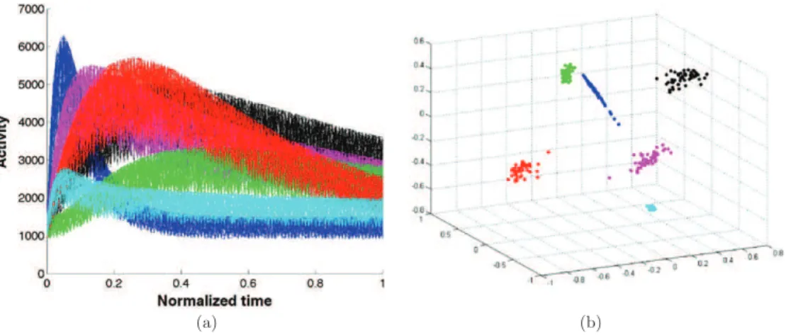
low-dimensional space. This changes the representation of the data points into axes where the clusters are best separated. As a last step, any conventional clustering algorithm can be used in this space where clusters can be more easily identified (Luxburg2007). In this work we used the classical KM algorithm as the last step to identify the clusters. To illustrate the principle of the proposed method, figure1(a) displays clusters composed of theoretical TACs discretized over 100 frames with added Gaussian noise. The initial 100-dimensional data (TACs) were first mapped into high-dimensional feature space and then the distances between the data were projected into a final low-dimensional space of dimension 6 given that six clusters were modeled. The representation of the clusters on the space spanned by the first three axes of the low-dimensional space is shown in figure1(b), where it can be observed that the embedded data clusters are well separated and easily identified.
2.2. Scale parameter analysis
Spectral clustering relies on the affinity matrix, and the Gaussian affinity scale parameter affects the quality of the clustering results because it conditions the separability between the clusters in the spectral embedding space and controls the affinity between the data (Ng et al2001). Several heuristic approaches were suggested to set this scale parameter. Brand and
(a) (b)
Figure 1.Illustration of spectral clustering on TACs affected by Gaussian noise. (a) Noisy TAC clusters in R100(100 time frames); (b) data representation in the first three dimension R3of the
spectral space showing the separation in the proposed final low-dimensional space.
Huang (2003) fixed σ as the mean of the distances between each point and its closest neighbor. Zelnik-Manor and Perona (2004) adopted a local point of view and defined for each point xia scale parameter σias the distance between the point xiand its seventh closest neighbor.
While for some applications these estimations might be correct, they might not always be optimal.
Rather than trying to automatically estimate the best value of σ , we propose to define an appropriate interval which the Gaussian scale parameter σ should belong to. This interval can be used to guide manual parameterization or to set research bounds of optimization methods. It is generally accepted that σ can be interpreted either as a threshold under which two points are considered similar or as a neighborhood radius (Luxburg2007). From this geometrical point of view, we estimate the upper and lower bounds of σ as some distances based on the TAC distribution.
We consider a limit case in which either all the points can be considered in the same cluster or each point in one distinct cluster. In other words, we start by considering an uniform TAC distribution in which all the TACs have the same neighborhood radius. By assuming that the p-dimensional data set is isotropic enough, we approximate the volume occupied by the whole data set S as a p-dimensional box bounded by the largest distance between all pairs of TAC in S. We then define the reference distance, noted Bmax, which separates all the TACs
with their closest neighbors, as follows:
Bmax=
max16i, j6nkxi−xjk
n1p
, (6)
where n and p are respectively the number and the dimension of the TAC.
Equation (6) means that a condition for some clusters to exist is that some TACs must be at a distance lower than a fraction of Bmax. Therefore we define Bmaxas an upper bound of the
interval for the scale parameter.
For the non-zero lower bound estimation, we consider the threshold under which the σ parameter does not affect the clustering result. This threshold, noted Bmin, is the lowest distance
between all pairs of TAC in S, calculated as follows: Bmin= min
By definition, the distance between all pairs of TACs is largest or equal than Bminso it does not
condition the separability between the clusters. For values of σ smaller than Bmin(σ < Bmin),
the Gaussian affinity matrix can be ill-conditioned and will not permit the extraction of dominant eigenvectors. The scale parameter σ should therefore be within this interval:
Bmin6σ 6Bmax. (8)
Note that these Bminand Bmaxbounds could be based on a theoretical study which links
the Gaussian affinity and the discretization of the heat kernel. This theoretical development shows that the Gaussian scale parameter should be within an appropriate interval in order to preserve the geometrical properties and thus the clustering quality (Mouysset et al2013).
3. Validation
3.1. Data simulation
The proposed clustering algorithm was evaluated using realistic PET images obtained from GATE Monte Carlo simulations (Jan et al2004, Jan et al2011).
3.1.1. TAC model. TACs were simulated based on the three compartment model proposed in (Maroy et al2008, Kamasak et al2005). This model assumes homogeneous vascular fraction in each considered region. The input function, corresponding to the molar concentration of the tracer in the plasma, is denoted CPand was given by:
CP(t ) = α0((α1t − α2− α3)e−λ1t+ α2e−λ2t+ α3e−λ3t). (9)
The kinetics of tissue compartment i, denoted Ciwere computed as:
Ci(t ) = Ã 3 X w=1 [ai,we−t/bi,w] ! ∗CP(t ), (10)
where ∗ denotes the convolution operator. The parameters α0, α1, α2, α3, λ1, λ2, λ3,ai,wand
bi,wwere randomly set using the constraints proposed in Maroy et al (2008).
3.1.2. Image simulation. We simulated dynamic PET images of the brain with GATE (Jan et al 2004, Jan et al 2011), using the Zubal head phantom as a voxelized source (Zubal et al1994). We simulated dynamic images as acquired using the Philips Gemini GXL PET scanner, with 20 frames (5 × 30 s followed by 15 × 60 s). Seven regions of the phantom were considered for image simulations: cerebellum, frontal lobes, occipital, thalamus, parietal lobes, remaining parts of the head, and air around the head, as shown in figure2(b). These regions were the ground truth for assessing the segmentation accuracy. Activities in all ROIs were simulated according to (10). Examples of simulated TACs for each ROI are shown in figure2(a). List-mode simulations were performed on a bi i7-980x computer with 12 cores and 48Go RAM. The total number of coincidences for each time frame varied between 8 and 70 millions. Corrections were applied for random and scattered coincidences. Reconstruction of the dynamic PET images was performed with an ANW-OSEM iterative method, using four iterations and 16 subsets, into voxels of 2.2 mm × 2.2 mm × 2.8 mm.
3.2. Clustering quality criteria
3.2.1. Quality of clustering. We measured the quality of clustering, denoted by Q, by estimating the Dice metric, which was calculated for every ROI as follows (Dice1945):
Q = 2card(Sres∩Struth) card(Sres) +card(Struth)
(a) (b)
Figure 2.(a) Example of simulated TACs used for our experiments. (b) ROIs of the Zubal head phantom used for PET image simulation.
where Sresand Struthare respectively the set of points of the clustering result and of the ground
truth.
3.2.2. TAC error. We calculated the root mean square error (Err) between the average TAC of identified clusters and the corresponding ground truth TACs used for the simulation:
Err =1 k k X c=1 s X xi∈Cc d(gc,xi)2 (12)
where Ccis the set of voxels clustered in class c, gcis the ground truth TAC of the corresponding
ROI, and d(gc,xi)is the distance between gcand a voxel xi∈Cc, as defined in (2).
3.3. Comparison with other segmentation methods
3.3.1. K-means. Wong et al (2002) introduced a KM clustering method to classify a number of tissue TACs as a function of their shape and magnitude into a smaller number of distinct classes that are mutually exclusive. The method is based on the RMSE defined by equation (12) to minimize the within-cluster sum of squares distances.
3.3.2. Hierarchical method. We used an agglomerative hierarchical clustering (HC) consisting in merging clusters iteratively as proposed by Guo et al (2003). The average linkage cluster method is used with a distance defined by:
8(l, m) =X i∈Cl X j∈Cm kxi−xjk2 NlNm (13)
where Cl and Cmare the lth and mth clusters respectively, and Nland Nmare the numbers of
data points in Cl and Cm. To avoid solutions in which a cluster would include a single data
point, k + 10 clusters were calculated (k being the number of clusters in the ground truth), and the smallest clusters were merged with the other clusters so as to maximize the quality of clustering Q.
3.3.3. Expectation-maximization. EM is a model-based approach in which clusters are represented as a parametric Gaussian distribution. The method consists in finding the parameters such as the fit between the data and the model is optimized. We used the maximum log-likelihood model proposed by Ashburner et al (1996).
(a) (b) (c) (d) (e) (f)
(g) (h) (i) (j) (k) (l)
Figure 3.Clustering results on axial and sagittal slices from simulated images. First row : axial slice. (a) Ground truth. (b) Sample frame of the simulated image. (c) KM. (d) HC. (e) EM clustering. (f) KSC. Second row: sagittal slice. (g) Ground truth. (h) Sample frame of the simulated image. (i) KM. (j) HC. (k) EM clustering. (l) KSC.
3.4. Demonstration of KSC on real dynamic PET images
We performed intrastriatal injections of quinolinic acid to achieve unilateral lesions of the left striatum of an adult Wistar rat. The injection of such exitotoxins into the brain causes marked gliosis and severe inflammation around the injection site (Isacson et al1987). The rat underwent dymanic microPET acquisitions with [18F]DPA-714, a radiotracer of the translocator protein (TSPO) which constitutes a biomarker for brain neuroinflammation. The dynamic acquisition consisted in a series of 27 frames of the following durations: 4 × 10, 4 × 20, 6 × 60, 10 × 80 and 3 × 600 s on a GE Explore Vista microPET/CT scanner. Images were reconstructed using a FORE+AWOSEM method (ten iterations, 16 subsets) with a voxel size of 0.39 × 0.39 × 0.78 mm3. Images of the brain were registrated into Paxinos coordinates in which an atlas can be
used to indicate the expected localization of the lesion. The atlas was merged and regularized, and then used as a mask to consider only the voxels inside the brain. We performed clustering of these registered dynamic scans into four ROIs with all the studied methods, expecting to find blood, specific uptake and non-specific gray matter and white matter uptakes. The segmentation results were visually analyzed for consistency as no gold standard was available.
4. Results
4.1. Clustering of realistic dynamic PET image simulations
Figure3displays representative results of the clustering obtained from the simulated dynamic PET images. In both rows, the first column contains the ground truth regions, the second column shows a simulated frame, and the last four columns show the results obtained with the four segmentation methods. All methods recovered most of the simulated regions. However, regions were more precisely delineated when using KSC compared to KM, HC and EM. In all cases the regions delineated by KSC were close to the corresponding ground truth, while this was not the case for other methods which yielded spurious regions. In particular, parietal and occipital regions of the sagittal slice (second row) were merged in the results obtained with KM and EM, and consequently the background was split in two regions. In the result obtained
(a) (b)
Figure 4.Affinity parameter bounds. (a) Percentage of clustering error against σ (semi-log scale). (b) Condition number of W against σ (log–log scale).
Table 1.Figures of merit characterizing the segmentation accuracy.
Zubal head
Method Q: axial(%) Err: axial Q: sagittal(%) Err: sagittal
KM 75 ± 18 0.21 ± 0.24 65 ± 20 0.41 ± 0.34
HC 68 ± 16 0.46 ± 0.34 66 ± 28 0.48 ± 0.47
EM 68 ± 18 0.34 ± 0.31 52 ± 23 0.80 ± 0.73
KSC 80 ± 9 0.16 ± 0.20 78 ± 14 0.28 ± 0.25
with HC the parietal region and background are merged, while all regions were correctly identified using KSC. It can also be noticed in the sagittal view that KSC is less sensitive to the variations in noise statistics along the axis of the scanner (top and bottom parts of the slice). While all methods were affected by PVE, KSC was less prone to create spurious regions in between two actual regions, except for the thalamus in figure3(l), which is surrounded by voxels associated to the frontal region.
Table1summarizes the quantitative results averaged over all ROIs and all slices of the simulated images. For each dynamic simulation, eight slices (four transverse and four sagittal slices) were individually processed. The quality of clustering measured by Q score (11) was significantly increased by KSC compared to the other methods, with global averaged scores of KSC of respectively 80% and 78% in axial and sagittal slices, with an increase between 6% and 33% compared to the three other methods. Such scores indicate accurate identification of the ROIs as the spatial resolution of the numerical phantom was intrinsically better than the one in the reconstructed PET images, leading to an expected loss of details in the reconstructed images. The error on TAC estimation was lower using KSC compared to KM, HC and EM, with a global reduction factor comprised between 1.3 and 2.8.
4.2. Scaling parameter bounds
To assess the bounds derived for the scale parameter σ , we measured two criteria against the value of σ used in KSC for the clustering of the noisy TACs presented in figure1(a). The supervised criterion Perroris the percentage of mis-clustered TACs. Figure4(a) displays
Perror for a representative case with k = 6 clusters, for values of σ ∈ [1e2 . . . 1e11] on a
(a) (b) (c) (d) (e) (f)
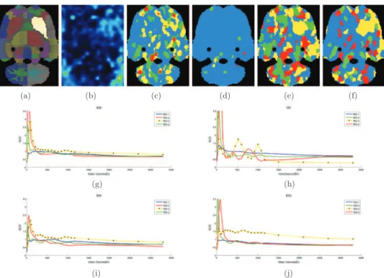
(g) (h)
(i) (j)
Figure 5.Clustering results on a real dynamic PET scan of a rat brain. First row: representative registered transverse slice. (a) Schiffer atlas. (b) Sample frame of the real image series. (c) KM (d) HC. (e) EM clustering. (f) KSC. Second and third rows: average TACs of the clustered ROIs. (g) KM. (h) HC. (i) EM clustering. (j) KSC.
are shown using dashed lines. For values of σ outside the proposed bounds, clustering errors occur, which was consistent with the theoretical bound estimates.
The second criterion is unsupervised, it is defined as the condition number of the affinity matrix W displayed in figure4(b). The values of the estimated lower bound Bmin and upper
bound Bmaxare shown in dashed lines. It can be observed that for values smaller than Bmin,
the normalized affinity matrix is ill-conditioned. With such high condition number, classical algorithms for estimating dominant eigenvectors of the affinity matrix cannot converge. These results explain the Perrorof 100% found for low values of σ in figure4(a).
4.3. Real dynamic PET data
Figure 5 displays representative results obtained with the four segmentation approaches. Figures5(a) and5(b) respectively present the Schiffer atlas (Schiffer et al2006) illustrating the expected location of the lesion and a representative frame (late frame with the highest SNR among the frames). Figures 5(c)–(f) display the results obtained with KM, HC, EM and KSC approaches. All methods except HC produced relatively large ROIs with one that could correspond to the region with specific uptake. The corresponding TACs of the four ROIs obtained with each method are presented in figures5(g)–(j). In the case of KSC, and to a lesser degree EM and KM, the four TACs could possibly correspond to an input function (ROI 2), brain with non-specific uptake merging white and grey matter (ROI 1), specific uptake (ROI 3) and a delayed input function (ROI 4). Identification of the corresponding physiological behaviors was more difficult for the TACs obtained with the HC method.
5. Discussion
We have described a new dynamic segmentation method, called KEC, to identify functional regions with similar TACs. The proposed method aims at overcoming some inherent limitations of conventional dynamic PET clustering. It is able to nonlinearly separate physiologically meaningful clusters in the time domain by mapping the data into a high dimensional space and then identifying the clusters in a low-dimensional space. KSC was compared to three other methods and presented improved segmentation performances. The method was shown to detect different kinetic behaviors and their associated ROIs. In the simulated brain data, no assumption was made on the anatomical structures nor on the pharmacokinetics of the tracer. No statistical model was needed as in the case of probabilistic methods like EM. The only pre-processing step consisted in simple thresholding to exclude voxels outside the head using the summed image over the entire acquisition.
In the experiments, the methods were applied on 2D+t slices because of the computational complexity of the matrix calculation involved in KSC. The computational cost of KSC is higher than other methods such as KM, as eigenvalues and eigenvectors of large matrix (size> 20 k × 20 k) have to be calculated. In this paper, all methods were implemented in MATLAB on a four cores, 12 Go RAM computer. Clustering of the entire volume was not possible with such implementation as it would require the storage and eigendecomposition of matrices of size larger than 5M × 5M. The specific mathematical approaches needed for such decompositions were not investigated in this work. For such 3D+t clustering, specific methods like Lanczos or Arnoldi algorithms can be implemented to handle the very large matrix computations. A fully 3D processing is expected to increase the robustness and facilitate the interpretation of the segmentation results. Alternative approaches include slice-by-slice clustering followed by cluster merging, or pre-clustering the data with fast linear methods (e.g. KM) to reduce the size of the data, followed by KSC segmentation. This was however not in the scope of the proposed paper.
The results presented in real microPET dynamic PET images are only qualitative as no ground truth was available. Future experimentations with arterial blood sampling are required to objectively assess the quality of real dynamic image clustering with KSC. The images were registered into Paxinos coordinates before the segmentation, which introduced an implicit regularization of the data that reduced the influence of noise in all methods. Three of the four methods produced an ROI that could correspond to the lesioned area. However, the lesion ROI obtained using KSC yielded a TAC that was more consistent with the expected kinetic in the lesion than the corresponding lesion TACs obtained using the EM or KM segmentation.
In this study, a weighting scheme proposed by Cheng-Liao and Qi (2010) was used to favor the influence of frames with reduced noise and better SNR. While it provided promising results, alternative weights can also be considered. Depending on the studied application and on the a priori knowledge available, it could improve the performance of KSC. For instance in some applications where a contrast between grey and white matter is normally expected (e.g. beta amyloid plaques in Alzheimer disease) it could be worth favoring the earliest and latest frames to benefit both from the difference between gray matter and white matter perfusion and from the specific uptake information, reducing the influence of middle frames where the TACs of grey and white matter cross.
The final step of the spectral clustering process involves a KM algorithm to cluster the data, but there is nothing principled about using the KM algorithm in this step (von Luxburg
2007). While initialization should be considered cautiously when KM is used directly on the data in their original Rpspace, the data resulting from the spectral clustering process should
contain well-distinct clusters. We project the data on the unity sphere on which the KM is initialized using the most distant centroids.
The number of clusters is generally unknown and is currently an input parameter of KSC. In this study, the correct number of clusters was systematically used, for the KM, EM and KSC methods. A higher number of clusters (k+10) was used for the hierarchical method as it tends to produce classes consisting of isolated points, and the classes were manually merged into the correct number of classes so as to maximize the quality of clustering. The estimation of the number of clusters is a general problem for all clustering algorithms and some methods have been designed that can be used with spectral clustering (Fraley and Raftery
2002, Still and Bialek2004, Luxburg2007). While this problem was not considered in this work, we are currently exploring the use of a specific matrix norm as an ad hoc indicator of both within-cluster and between-cluster similarities to automatically estimate the number of classes.
In dynamic PET images, the TACs of voxels within a functional ROI are not exactly behaving the same and a variety of TACs can be observed within a functional ROI. These differences in TAC come from several factors among which the local variations in the radiotracer target density, the PVE that produces a mixture of kinetics on the borders of adjacent ROIs, and the level of noise. In the Rp space of TACs, such factors spread the
clusters away from their centroids. In KSC, as in the other three segmentation methods, there is no implicit assumption regarding the presence or absence of such spreading. These methods aim at generating the clusters that are as much different to each other as possible, and as homogeneous as possible within a cluster, implicitly allowing for some spreading. However, the TAC behavior affects the quality of clustering when kinetic profiles overlap too much between functional ROIs. The reconstruction parameters that have an influence on this spreading (number of iterations, corrections, voxel size, frame durations, regularization to cite a few) should be optimized if KSC is used in clinical applications. While the PVE issue could be reduced by PVE correction methods, we did not use any in this study. The relatively good behavior of KSC can be explained by the fact that it makes no assumption regarding the shape of the clusters in the projection space. Among other undesirable artifacts that can alter the segmentation process, physiological motions can severely impact the kinetics measured in each voxel. In this study we focused on brain imaging for which motion artifacts are less frequent, but when applicable, movement correction methods should be used.
The proposed algorithm does not account for the spatial coordinates of the voxels, as none of the three compared methods. The comparative evaluation of the methods therefore tested their effectiveness in the feature selection process. Incorporating spatial information would likely reduce the sensitivity of the method to noise and increase its robustness (Chen et al
2001). In KSC, it can be performed by adding a spatial distance term within the Gaussian kernel (Shi and Malik2000), or by including the coordinate information as part of the features. However, in both cases it would introduce an additional parameter (or equivalently a choice in the coordinate system) to control the tradeoff between the terms related to the distance between kinetics and the term describing the spatial distance between voxels. In brain imaging, some disconnected regions can have the same kinetics hence spatial constraints might be difficult to optimize. Further developments are required to include a spatial term in KSC.
KSC can be used as a pre-processing step before kinetic analysis to increase the signal-to-noise ratio. It is based on the differences in the voxel kinetics, which is the same type of information used to calculate parameters of compartmental models. These models produce parametric images, like binding potential maps. KSC could increase the robustness of quantification by providing a reliable segmentation yielding ROIs with similar TACs that can then be averaged or further manipulated. Supervised approaches have been proposed and
successfully applied to the study of neuroinflammation where no reference region is devoid of the TSPO, using [11C]PK1195 (Turkheimer et al2007, Yaqub et al2012). They consist in predetermining kinetic classes that correspond to the expected TACs behavior and to estimate in each voxel the contribution of each of these classes. The definition of the kinetic classes currently relies on MRI segmentation and could benefit from KSC to define ROIs with distinct kinetic profiles without anatomical priors.
6. Conclusion
We have proposed an approach based on spectral clustering for the segmentation of dynamic PET images. In KSC, the kinetic data is mapped into a high dimensional space and then embedded into a low-dimensional space which increases the separability of the clusters and makes KSC able to handle clusters that have arbitrary shapes in the feature space. We proposed an estimation of the bounds of the scale parameter involved in the clustering process. We showed experimental results on GATE Monte Carlo simulations and real dynamic PET images which confirmed the improvement obtained in ROI delineation compared to three other segmentation methods. As a result, KSC appears as a promising pre-processing tool before parametric map calculation or ROI-based quantification tasks.
Acknowledgments
The research leading to these results has received funding from the European Union’s Seventh Framework Programme (FP7/2007-2013) under grant agreement no HEALTH-F2-2011-278850 (INMiND), the Lebanese University, Hadath, Lebanon and from the Lebanese CNRS, Beirut, Lebanon.
References
Ashburner J, Haslam J, Taylor C, Cunningham V and Jones T 1996 A cluster analysis approach for the characterization of dynamic PET data Quantification of Brain Function using PET ed R Myers, V Cunningham, D Bailey and T Jones (San Diego, CA: Academic) pp 301–6
Belkin M and Niyogi P 2002 Laplacian eigenmaps and spectral techniques for embedding and clustering (Advances
in Neural Information Processing Systemsvol 14) ed T Leen, T Dietterich and V Tresp (Cambridge, MA: MIT Press) pp 585–91
Bengio Y, Delalleau O, Le Roux N, Paiement J, Vincent P and Ouimet M 2004 Learning eigenfunctions links spectral embedding and kernel PCA Neural Comput.162197–219
Brand M and Huang K 2003 A unifying theorem for spectral embedding and clustering Proc. 9th Int. Workshop on
Artificial Intelligence and Statisticsed C Bishop and B Frey (abstract 189)
Brankov J, Galatsanos N, Yang Y and Wernick M N 2003 Segmentation of dynamic PET or fMRI images based on a similarity metric IEEE Trans. Nucl. Sci.501410–14
Chen J, Gunn S and Nixon M 2001 Markov random field models for segmentation of PET images Information
Processing in Medical Imaging (Lecture Notes in Computer Sciencevol 2082) (Berlin: Springer)pp 468–74
Cheng-Liao J and Qi J 2010 Segmentation of mouse dynamic PET images using a multiphase level set method Phys.
Med. Biol.556549–69
Ciarlet P 1978 The Finite Element Method For Elliptic Problems (Amsterdam: North-Holland)
Dhillon I, Guan Y and Kulis B 2007 Weighted graph cuts without eigenvectors: a multilevel approach IEEE Trans.
Pattern Anal.291944–57
Dice L 1945 Measures of the amount of ecologic association between species Ecology26297–302
Filippone M, Camastra F, Masulli F and Rovetta S 2008 A survey of kernel and spectral methods for clustering
Pattern Recognit.41176–90
Fraley C and Raftery A 2002 Model-based clustering, discriminant analysis, and density estimation J. Am. Stat.
Frouin F, Boubacar P, Frouin V, De Cesare A, Todd-Pokropek A, Merlet P and Herment A 2001 3-D Regularisation and segmentation of factor volumes to process PET H215O myocardial perfusion studies Functional Imaging
and Modelling of the Heart (Lecture Notes in Computer Sciencevol 2230) ed T Katila, J Nenonen, I E Magnin, P Clarysse and J Montagnat (Berlin: Springer)pp 91–6
Guo H, Renault R, Chen K and Reiman E 2003 Clustering huge data sets for parametric PET imaging
Biosystems7181–92
Hirsch F and Lacombe G 1999 Elements of Functional Analysis (Berlin: Springer)
Isacson O, Fischer W, Wictorin K, Dawbarn D and Bjorklund A 1987 Astroglial response in the excitotoxically lesioned neostriatum and its projection areas in the rat Neuroscience201043–56
Jan S et al 2004 GATE: a simulation toolkit for PET and SPECT Phys. Med. Biol.494543–61
Jan S et al 2011 GATE V6: a major enhancement of the GATE simulation platform enabling modelling of CT and radiotherapy Phys. Med. Biol.56881–901
Kamasak M 2009 Clustering dynamic PET images on the Gaussian distributed sinogram domain Comput. Methods
Programs Biomed.93217–27
Kamasak M, Bouman C, Morris E and Sauer K 2005 Direct reconstruction of kinetic parameter images from dynamic PET data IEEE Trans. Med. Imaging24636–50
Kimura Y, Senda M and Alpert N 2002 Fast formation of statistically reliable FDG parametric images based on clustering and principal components Phys. Med. Biol.47455–68
Krak N, Boellaard R, Hoekstra O, Twisk J, Hoekstra C and Lammerstma A 2005 Effects of ROI definition and reconstruction method on quantitative outcome and applicability in a response monitoring trial Eur. J. Nucl.
Med. Mol. Imaging32294–301
Krestyannikov E, Tohka J and Ruotsalainen U 2006 Segmentation of dynamic emission tomography data in projection space Computer Vision Approaches to Medical Image Analysis (Lecture Notes in Computer science vol 4241) ed R Beichel and M Sonka (Berin: Springer)pp 108–19
Luxburg U 2007 A tutorial on spectral clustering Stat. Comput.17395–416
Maroy R et al 2008 Segmentation of rodent whole-body dynamic PET images: an unsupervised method based on voxel dynamics IEEE Trans. Med. Imaging27342–54
Mouysset S, Noailles J, Ruiz D and Tauber C 2013 Spectral Clustering: interpretation and Gaussian parameter
Studies in Classification, Data Analysis and Knowledge Organizationed H Bock, W Gaul, M Vichi and C Weihs (Berin: Springer)
Ng A, Jordan M and Weiss Y 2001 On Spectral Clustering: Analysis And An Algorithm (Advances in Neural
Information Processing Systemsvol 14) ed M Jordan, Y LeCun and S Solia (Cambridge, MA: MIT Press) 849–56
Qi J and Leahy R M 1999 A theoretical study of the contrast recovery and variance of MAP reconstructions from PET data IEEE Trans. Med. Imaging18293–305
Shawe-Taylor J and Cristianini N 2004 Kernel Methods for Pattern Analysis (New York: Cambridge University Press) Shi J and Malik J 2000 Normalized cuts and image segmentation IEEE Trans. Pattern Anal.22888–905
Schiffer W, Mirrione M, Biegon A, Alexoff D, Patel V and Dewy S 2006 Serial micropet measures of the metabolic reaction to a microdialysis probe implant J. Neurosci. Methods155272–84
Still S and Bialek W 2004 How many clusters? Neural Comput.162483–506
Turkheimer F E, Edison P, Pavese N, Roncaroli F, Anderson A N, Hammers A, Gerhard A, Hinz R, Tai Y F and Brooks D J 2007 Reference and target region modeling of [11C]-(R)-PK11195 brain studies J. Nucl. Med.
48158–67
Wong K, Feng D, Meikle S and Fulham M J 2002 Segmentation of dynamic PET images using cluster analysis IEEE
Trans. Nucl. Sci.49200–7
Yaqub M, van Berckel B N, Schuitemaker A, Hinz R, Turkheimer F E, Tomasi G, Lammertsma A A and Boellaard R 2012 Optimization of supervised cluster analysis for extracting reference tissue input curves in (R)-[(11)C]PK11195 brain PET studies J. Cereb. Blood Flow Metab.321600–8
Zelnik-Manor L and Perona P 2004 Self-Tuning Spectral Clustering (Advances in Neural Information Processing
Systemsvol 17) ed L Saul, Y Weiss and L Bottou (Cambridge, MA: MIT Press) pp 1601–8
Zhou Y 2000 Model fitting with spatial constraint for parametric imaging in dynamic PET studies PhD Thesis UCLA Zubal G, Harrell C, Smith E, Rattner Z, Gindi G and Hoffer P 1994 Computerized three-dimensional segmented