HAL Id: hal-00881484
https://hal.archives-ouvertes.fr/hal-00881484v2
Submitted on 4 Mar 2015
HAL is a multi-disciplinary open access
archive for the deposit and dissemination of
sci-entific research documents, whether they are
pub-lished or not. The documents may come from
teaching and research institutions in France or
abroad, or from public or private research centers.
L’archive ouverte pluridisciplinaire HAL, est
destinée au dépôt et à la diffusion de documents
scientifiques de niveau recherche, publiés ou non,
émanant des établissements d’enseignement et de
recherche français ou étrangers, des laboratoires
publics ou privés.
New estimators and guidelines for better use of fetal
heart rate estimators with Doppler ultrasound devices
Iulian Voicu, Sébastien Ménigot, Denis Kouamé, Jean-Marc Girault
To cite this version:
Iulian Voicu, Sébastien Ménigot, Denis Kouamé, Jean-Marc Girault. New estimators and guidelines
for better use of fetal heart rate estimators with Doppler ultrasound devices. Computational and
Mathematical Methods in Medicine, Hindawi Publishing Corporation, 2014, vol. 2014 (Article ID
784862), pp. 1-10. �10.1155/2014/784862�. �hal-00881484v2�
O
pen
A
rchive
T
OULOUSE
A
rchive
O
uverte (
OATAO
)
OATAO is an open access repository that collects the work of Toulouse researchers and
makes it freely available over the web where possible.
This is an author-deposited version published in :
http://oatao.univ-toulouse.fr/
Eprints ID : 12757
To link to this article : DOI :10.1155/2014/784862
URL :
http://dx.doi.org/10.1155/2014/784862
To cite this version : Voicu, Iulian and Ménigot, Sébastien and
Kouamé, Denis and Girault, Jean-Marc
New estimators and guidelines
for better use of fetal heart rate estimators with Doppler ultrasound
devices
. (2014) Computational and Mathematical Methods in
Medicine, vol. 2014. pp. 1-10. ISSN 1748-670X
Any correspondance concerning this service should be sent to the repository
administrator:
staff-oatao@listes-diff.inp-toulouse.fr
Research Article
New Estimators and Guidelines for Better Use of Fetal Heart
Rate Estimators with Doppler Ultrasound Devices
Iulian Voicu,
1,2Sébastien Ménigot,
1,2Denis Kouamé,
3and Jean-Marc Girault
1,21Signal & Imaging Group, University Franc¸ois Rabelais of Tours, PRES Loire Valley University, UMR INSERM U930,
7 Avenue Marcel Dassault, 37200 Tours Cedex, France
2Inserm, U930, 10 Boulevard Tonnell´e, BP 3223, 37032 Tours Cedex, France
3IRIT UMR 5505, Universit´e Paul Sabatier Toulouse 3, 118 Route de Narbonne, 31062 Toulouse Cedex 9, France
Correspondence should be addressed to Jean-Marc Girault; jean-marc.girault@univ-tours.fr
Characterizing fetal wellbeing with a Doppler ultrasound device requires computation of a score based on fetal parameters. In order to analyze the parameters derived from the fetal heart rate correctly, an accuracy of 0.25 beats per minute is needed. Simultaneously with the lowest false negative rate and the highest sensitivity, we investigated whether various Doppler techniques ensure this accuracy. We found that the accuracy was ensured if directional Doppler signals and autocorrelation estimation were used. Our best estimator provided sensitivity of 95.5%, corresponding to an improvement of 14% compared to the standard estimator.
1. Introduction
Continuous monitoring of fetal parameters has shown their advantages in estimating fetal wellbeing [1]. According to the report of the Society for Maternal-Fetal Medicine [2], continuous fetal heart rate monitoring has reduced infant mortality. The development or the improvement of nonin-vasive methods dedicated to continuous fetal monitoring is therefore of major interest.
One important parameter in assessing fetal wellbeing is the variability of the fetal heart rate. This parameter, which corresponds to the variation between intervals of two consecutive heart beats, is an indicator of central nervous system development [3–5]. It characterizes fetal behavior states [6–8] and can be an indicator of further neurological evolution [9]. Variability analysis provides a good indication of fetal distress [10] and identifies fetuses with intrauterine growth retardation [11]. According to Dawes criteria [12], variability of 4 ms is a predictor of the lack of acidosis, while a value of 2.6 ms is critical for the fetus. In the normal fetal heart rate range (110–160 bpm), a time variability of 4 ms corresponds to a cardiac frequency variability of 0.81 bpm, while a time variability of 2.6 ms corresponds to a cardiac
frequency variability of 0.53 bpm (the values of 0.53 bpm and 0.81 bpm are obtained as follows:60/(60/110−2.6 ms)−110 = 0.56 bpm and 60/(60/110 − 4.0 ms) − 110 = 0.81 bpm, resp.). Other authors [13] suggest that it is necessary to estimate the heart rate with an accuracy of 0.25 bpm in order to analyze fetal heart rate variability correctly. Reliable estimation of fetal heart rate and hence of heart rate variability is therefore essential.
Several methods are available to assess the fetal heart rate. These methods differ both at the Doppler signal level (directional or nondirectional) and at the level of the algo-rithm that estimates the heart rate. For example, existing devices on the market such as Sonicaid Oxford (Oxford Sonicaid Instruments, Abington, UK) [14], Hewlett-Packard 8030A (Hewlett-Packard, Palo Alto, CA, USA) [15], and Philips Avalon F40 (Philips, Amsterdam, Netherlands) use the envelope of the nondirectional Doppler signal. Other authors [16, 17] have used the envelope of the directional Doppler signal. Several algorithms based on autocorrelation are commonly used to estimate the heart rate (Oxford Sonicaid, Hewlett-Packard 8030A, and Philips Avalon F40). These algorithms have been applied either directly to the Doppler signal envelope (directional or nondirectional) or to
the signals resulting from discrete wavelet decomposition of the envelope. In the latter case, the final estimated heart rate involves the combination of different estimates [16].
In this study, we first verified whether the pulsed Doppler techniques currently used in commercial devices ensure such an accuracy of 0.25 bpm, and we propose here some recom-mendations regarding parameter settings. We also compared the techniques used in commercial devices with other pulsed Doppler techniques that use directional Doppler signals. We evaluated the efficacy of all these techniques empirically (error of estimation of the fetal heart rate, sensitivity, and false negative rate).
The originality of this study lies in the recommendations on the parameter settings of the system and in the description of the individual limitations of each technique. Finally, to improve detection probability, a new method based on the combination of heart rates obtained from directional signals is proposed.
2. Materials and Methods
In this section, we describe the Doppler system we developed, the patients, and the synthetic signals used for the compar-ison of each estimator. The synthetic signals were inferred from real signals. Finally, we present the various existing techniques for estimation of fetal heart rate and we present a new technique based on a combined procedure.
2.1. The Doppler System. In order to evaluate fetal wellbeing objectively and to classify the fetus, we codeveloped the pulsed, multitransducer, multichannel Doppler Actifoetus unit with Altha¨ıs Technologies (Tours, France).
Our system comprised a personal computer (PC) and our Actifoetus unit. The Actifoetus unit contained three groups of four transducers and a Doppler acquisition board. The detailed operating functions of the acquisition board were presented in [18].
The transducers exploring the fetal heart were non-focused and monoelement. They were circular in shape, with a diameter of 13.5 mm and an acoustic power of 1 mW/cm2. Geometrically, the transducers were located at the center of gravity and at the top of an equilateral triangle with sides measuring 40.7 mm.
The transducers were placed on the mother’s abdomen. They transmitted a sinusoidal pulse at 2.25 MHz with a pulse repetition frequency (PRF) of 1 kHz. Note that a theoretical
accuracy of 60/2/1000 = 0.03 bpm can be achieved with
this value of 1 kHz and accuracy can be still further improved by performing interpolation of the correlation function. The wave was propagated through the mother’s abdomen towards the fetal heart. The backscattered signal was recorded from five different depths, annotated 𝐷1, . . . , 𝐷5. Note that only one channel was considered in the present study.
The ultrasound signal received was converted into an electrical signal and amplified to compensate for the atten-uation of 1 dB/cm/MHz. The signal was then demodulated in phase (𝐼) and quadrature (𝑄) [19]. After demodulation,
150 120 90 60 30 0 0 100 200 300 400 500 600 700 800 900 1000 Time (ms) A m p li tu d e
Rectified nondirectional signal
Envelope of the rectified nondirectional signal
(a) Envelope of the real nondirectional Doppler signal
−30 −60 −90 −120 −150 150 120 90 60 30 0 0 100 200 300 400 500 600 700 800 900 1000 Time (ms) A m p li tu d e xB xF
(b) Envelopes of real directional signals
Figure 1: A real Doppler signal (PRF = 1 kHz) of 1000 ms, recorded with the second transducer in the fourth-channel: (a) Doppler signal (dashed line) and its envelope (solid line); (b) the envelopes of directional signals corresponding to ultrasound scatters approaching to the transducer (solid line) and moving away from the transducer (dash-dot line), respectively.
the signals were digitized. The digital outputs of the convert-ers represented the digital Doppler signal.
2.2. Patients. The Doppler signals were acquired at the CHRU “Bretonneau” Tours, France. The consent of each patient was obtained and the study was approved by the Ethics Committee of the Clinical Investigation Centre for Innovative Technology of Tours (CIC-IT 806 CHRU of Tours). Patients were older than eighteen years and all pregnancies were single. The recordings were made during the twenty-fifth and fortieth gestational weeks. Evolution during pregnancy was normal for all fetuses.
2.3. Simulation. Because it was difficult to quantify the effec-tiveness of the estimation techniques directly on real signals and because there was no suitable model, we generated syn-thetic signals. These synsyn-thetic signals were used as a ground-truth to evaluate the effectiveness of each estimator. To make these signals as realistic as possible, we proceeded in two stages: an analyzing stage deducing the characteristics of the real Doppler signal envelope and a synthetic phase providing realistic simulated signals. Figures 1(a) and 1(b) show 1000 ms of the envelope of a real nondirectional Doppler signal
300 250 200 150 100 50 0 4 2 4 3 .24 4 3 .3 1 4 3 .4 2 4 3 .6 3 4 3 .7 1 4 4 100 50 0 43.2 43.6 dM2M1 dM4M3 dM1M4 M1 M2 M3 M4 dP1P2 dP2P3 dP3P4 Time (s) Time (s) A m p li tu d e A m p li tu d e T m Ts PA PP P1 P2 P3 P4
Figure 2: Envelope of a real directional Doppler signal of 2000 ms. The parameters defining the synthetic signal are the amplitudes and durations of peaks, the lag, and the differences in amplitude of two consecutive peaks over time.
and the two envelopes of corresponding directional signals obtained from the 𝐼 and 𝑄 signals [19, 20]. The synthetic envelope signal was calculated as follows:
𝑥𝑒(𝑡) = 𝑥𝐵(𝑡) + 𝑥𝐹(𝑡) , (1)
where 𝑥𝐵(𝑡) and 𝑥𝐹(𝑡) are the envelopes of directional Doppler signals produced by the scatters that approach and move away from the transducer, respectively.
We verified (Figures 1(a) and 1(b)) that the envelope of the real nondirectional Doppler signal had the signatures of both envelopes of the directional signals. For example, at around 500 ms, the envelope of the nondirectional signal was mainly influenced by scatters that approached the transducer, while at around 400 ms, we observed the influence of movements away from the transducer. The alternating influence of these two movements determined the envelope of the nondirec-tional signal.
2.3.1. Analysis of Real Directional Signals. Figure 2 shows 2000 ms of the envelope of a real directional Doppler signal. In order to find the important parameters required for the synthesis of this signal, we extracted its intrinsic features (the number and amplitudes of the peaks, the lags between the peaks, and the differences in amplitude between the peaks). The values of these parameters were evaluated by considering a quasiconstant fetal heart rate.
Figure 2 represents a sequence of several patterns. These patterns were made up of peaks that corresponded to cardiac wall and valve movements of the fetal heart. As suggested by Shakespeare et al. [21], although six peaks (atrial contraction, ventricular contraction, opening and closing of the mitral valves, and opening and closing of the aortic valves) could be detected theoretically, only a few peaks were in practice detected in the nondirectional Doppler signal. From our
analysis, it appeared that the most likely pattern was that with four peaks. Note that this signature composed of four peaks could vary considerably from one beat to another, and it was similar to that identified by Jezewski et al. [13]. Among all these patterns, the most likely was the pattern with peaks in the order 2143; that is, the highest peak
𝑀1 was in second position, the second highest peak 𝑀2
was in first position, and so forth. For the 2143-pattern, we evaluated the amplitudes of each peak (𝑀1, 𝑀2, 𝑀3, and 𝑀4), the peak durations (𝑇1, 𝑇2, 𝑇3, and𝑇4), the lags between two consecutive peaks (𝑑𝑃1𝑃2,𝑑𝑃2𝑃3, and𝑑𝑃3𝑃4), and the differences in amplitude between two consecutive peaks (𝑑𝑀2𝑀1, 𝑑𝑀1𝑀4, and 𝑑𝑀4𝑀3). The results of this statistical analysis are reported in Table 1.
As the patterns observed in Figure 2 were noisy, we decided to assess the noise level in order to simulate noisy synthetic Doppler signals. We assessed the signal to noise ratio (SNR) as follows:
SNR= 10 ⋅ log10(𝑃𝐴
𝑃𝑃) , (2)
where𝑃𝐴 and𝑃𝑃 are the powers of the active and passive regions, respectively. We considered the active region as the area containing the pattern peaks, whereas there were none in the passive region. Using (2), we found that the SNR calculated on our real signals corresponded to a Gaussian law: SNR∼N (11, (√2.5)2(dB)).
2.3.2. Synthesis of Synthetic Directional Signals. Analysis of the envelope of directional signals showed the presence of four peaks, which appeared in order 2143 inside the periodic patterns. The synthesis of such a signal must account for
Actifoetus unit
Detection of the envelopes of the
directional signal
Fetal heart rate detection
Fetal heart rate detection
Fetal heart rate detection
Fetal heart rate detection
Fetal heart rate detection
Fetal heart rate detection
Combination Combination nondirectional and I1and algorithm I2and algorithm I1and algorithm I2and algorithm I1and algorithm I2and algorithm E1 E2 E3 E4 E5 E6 E7 E8 xF xB xe I Q
Figure 3: General diagram of the Doppler data processing acquired using one transducer and one channel.𝑥𝐹and𝑥𝐵represent the envelopes of the directional signals, and𝑥𝑒represents the envelope of the nondirectional signal.𝐼1,𝐼2are the two autocorrelation estimators.
Table 1: Statistics evaluated using (2143) patterns: 𝑀𝑖 represents the statistics of the maxima, where 𝑖 = 1, . . . , 4, 𝑑𝑃1𝑃2, 𝑑𝑃2𝑃3, 𝑑𝑃3𝑃4 represent the differences between the positions of two
adjacent maxima over time; 𝑑𝑀2𝑀1,𝑑𝑀1𝑀4,𝑑𝑀4𝑀3 represent statistical differences between two adjacent maxima over time, and 𝑇 represents the statistics of the peak durations. We found that the statistics of the four peaks of𝑇𝑖,𝑖 = 1, . . . , 4, were identical.
Law Gaussian Uniform 𝑀1 89.06 ± 31.48 𝑀2 69.70 ± 21.84 𝑀3 54.80 ± 19.21 𝑀4 36.28 ± 18.28 𝑑𝑀2𝑀1 (5–50) 𝑑𝑀1𝑀3 (5–50) 𝑑𝑀3𝑀4 (5–40) 𝑑𝑃1𝑃2 41.50 ± 18.18 𝑑𝑃2𝑃3 92.92 ± 27.76 𝑑𝑃3𝑃4 47.81 ± 30.09 𝑇 (ms) (25–45)
these characteristics. Equation (3) shows the two possible components of such a signal:
𝑥𝐵(𝑡) = { { { { { { { { { 𝑏 (𝑡) +∑4 𝑖=1𝑀𝑖 sin(2𝜋𝑓𝑖(𝜃 + 𝑇𝑖 2 ))Rect𝑇𝑖(𝜃) , ∀𝑡 ∈ [0, 𝑇𝑚] , 𝑏 (𝑡) , ∀𝑡 ∈ (𝑇𝑚, 𝑇𝑠] , (3)
where 𝑏(𝑡) is the noise, 𝑀𝑖 is the peak amplitude, 𝑓𝑖 = 1/(2𝑇𝑖) is the peak frequency, Rect𝑇𝑖(𝜃) is the unit rectangular function centered on𝑇𝑐𝑖with width𝑇𝑖and𝜃 = 𝑡 − 𝑇𝑐𝑖,𝑇𝑚is the pattern duration, and𝑇𝑠is the synthetic signal period. We set a constant interval𝑇𝑠between the highest peaks of two consecutive patterns of the synthetic signal, as illustrated in Figure 2. We also chose the𝑇𝑚 pattern period as 50% of the synthetic cardiac cycle period𝑇𝑠, since this period can vary between 40 and 60% [22].
Using (3), we generated two synthetic noisy envelopes corresponding to the envelopes of the directional signals. The envelope of the nondirectional synthetic signal was modeled using (1), being the sum of the envelopes of the both directional synthetic signals. In order to simplify our study, only𝑥𝐵(𝑡) was calculated, 𝑥𝐹(𝑡) being a delayed and amplified version of𝑥𝐵(𝑡). To simulate realistic signals, we introduced a lag𝜏 between the directional components:
𝑥𝐹(𝑡) = 𝛼𝑥𝐵(𝑡 − 𝜏) , (4)
where𝑥𝐹(𝑡) and 𝑥𝐵(𝑡) are the envelopes of directional signals and 𝜏 is the lag between the two envelopes. 𝛼 is a factor that represents the amplitude ratio between the two types of envelope. From Figure 1,𝜏 ≈ 40 ms and 𝛼 ≈ 2.
2.4. Estimators. In this section, we describe the different estimators used in our study. Each estimator that was based on the autocorrelation function was denoted by 𝐸𝑖, 𝑖 = 1, . . . , 8, as illustrated in Figure 3. Each estimator operated on different signals:𝑥𝐹(𝑡), 𝑥𝐵(𝑡), and 𝑥𝑒(𝑡).
Devices existing on the market currently use the𝑥𝑒(𝑡) envelope and autocorrelation. The estimators that used these configurations were𝐸7and𝐸8. The mathematical expression
of the two autocorrelation estimators is given in [23] and is represented thereafter by 𝐼1(𝑡, 𝑘) = 1𝑊 𝑊−|𝑘|−1 ∑ 𝑛=0 𝑥 (𝑡, 𝑛) ⋅ 𝑥 (𝑡, 𝑛 + 𝑘) ; 𝐼2(𝑡, 𝑘) = 1𝑊 𝑊−1 ∑ 𝑛=0𝑥 (𝑡, 𝑛) ⋅ 𝑥 (𝑡, 𝑛 + 𝑘) , (5)
where𝑊 is the size of the analyzing window, 𝑡 is the time for which the estimator is computed, and 𝑘 is the lag. 𝑥(𝑡) represents one of the signals analyzed (𝑥𝐹(𝑡), 𝑥𝐵(𝑡), or 𝑥𝑒(𝑡)). We tested other estimators (𝐸1, . . . , 𝐸6) which used direc-tional signals𝑥𝐹(𝑡) and 𝑥𝐵(𝑡), together with 𝐼1and𝐼2. 2.4.1. Algorithm. The algorithm to estimate the fetal heart rate was the same for all three signals (𝑥𝑒(𝑡), 𝑥𝐹(𝑡), and 𝑥𝐵(𝑡)). The steps of the algorithm were as follows.
(1) Extract from each signal under consideration (𝑥𝑒(𝑡), 𝑥𝐹(𝑡), or 𝑥𝐵(𝑡)) a limited number 𝑊 of samples, 𝑊 being the window size.
(2) Compute𝐼1(𝑊) and 𝐼2(𝑊).
(3) Using an empirical threshold, detect the position of𝑁 peaks in 𝐼1(𝑊) and 𝐼2(𝑊).
(4) From the position of𝑁 peaks of 𝐼1(𝑊) and 𝐼2(𝑊),
determine the durations 𝐷𝑖 between consecutive
peaks with𝑖 = 1, 2, . . . , 𝑁 − 1.
(5) Calculate the𝑁 − 1 cardiac frequencies with CF𝑖 = 60/𝐷𝑖, 𝑖 = 1, 2, . . . , 𝑁 − 1. This conditional test
limits the number of cardiac frequencies CF𝑖 esti-mated from 𝐼1 or 𝐼2 in the average computation. This conditional test also permits removal of cardiac frequency estimates that are half the expected value, as are sometimes observed (Shakespeare et al. [21]). (6) Calculate the average cardiac frequency (FHR) from
CF𝑖not exceeding 35 bpm [13]: FHR= 1 𝑁 − 1 𝑁−1 ∑ 𝑖 CF𝑖. (6)
As an illustration, consider a window of4.096 s. Whenever the cardiac frequency was240 bpm, 16 peaks were observed in the autocorrelation function. Using an empirically set threshold, the duration between each peak was measured (𝐷1 = 0.250 s, . . . , 𝐷15 = 0.250 s) and cardiac frequencies of CF1 = 60/0.250 bpm, . . . , CF15 = 60/0.250 bpm were estimated. The average cardiac frequency was obtained by FHR = (1/15) ∑15𝑖 CF𝑖 = 240 bpm. Note that 4 peaks were observed with60 bpm and 𝐷1 = 60/1.0 = 1.0 s, . . . , 𝐷3 = 60/1.0 = 1.0 s were estimated. The average cardiac frequency was obtained by FHR= (1/3) ∑3𝑖CF𝑖= 60 bpm.
Thus the proposed algorithm correctly worked in the range of 60–240 bpm. However, the standard deviation of the FHR estimation was not the same for its extreme values since in one case the average was obtained with three values
whereas the average was obtained with fifteen values in the other.
Note that such an algorithm is not perfect since it is hypothesised that the FHR is constant during the process. Sometimes the second peak of the autocorrelation can be lower than the third and the FHR estimate is incorrect. A process must be performed to remove outliers.
2.4.2. Elimination of Outliers. In order to eliminate outlier estimates associated with estimator dysfunction, we intro-duced a postprocessing step. This postprocessing step was applied only in the case of real signals. An estimate was con-sidered to be an outlier if it laid outside the statistic computed from 40 previous estimates, or if it differed between two consecutive analysis windows by 35 bpm.
2.4.3. Combination. In order to improve the effectiveness of the FHR estimation, we combined estimations. For𝐸2and𝐸5, the two values of the fetal heart rate estimated on signals𝑥𝐹(𝑡) and𝑥𝐵(𝑡) were combined. The estimate on the two signals was achieved using𝐼1or𝐼2. The combination rule we used was as follows:
(i) if the heart rate was detected on a single signal, the combined value took this value;
(ii) if the heart rate was detected on both signals, the combined value was the average of the two values. Note that, in contrast to Kret’s study [16], we combined the fetal heart rates estimated on both directional Doppler signals, while Kret’s technique was based on combination of fetal heart rate estimations computed after discrete wavelet decomposition of the envelope of the directional Doppler signal. Since Kret’s technique was applied only for continuous Doppler signals, it was not taken into consideration in our study.
3. Results
To find the best estimators and the conditions in which they could be used, we performed a series of simulations and experiments. Using simulations, we sought configurations that ensured an error of estimation, that is, the expected accuracy below 0.25 bpm, the highest sensitivity, and the lowest false negative rate. Experimentally, we sought the best configuration for optimal use of the estimator.
3.1. Simulated Signals. We present the results from two types of simulation. In the first series of simulations, we sought parameter settings that ensured the desired accuracy of 0.25 bpm. In the second series of simulations, we evaluated the effectiveness of each estimator in terms of true positive rate and false negative rate.
3.1.1. Optimal Parameter Settings. The results presented in Figures 4 and 5 were obtained for synthetic signals of 30 s. The parameters that varied in our analysis were the periodicity of the signal𝑇𝑠, the SNR, the window size𝑊, and the lag
60 75 100 120 150 200 240 0 500 1000 1500 2000 2500 3000 3500 4000 4500 5000 Frequency (bpm) D u ra ti o n (m s) 3584 4096
Duration of the analyzing window for 𝜏 = 0 ms
E4 E1 E7 E2 (a) 60 75 100 120 150 200 240 0 500 1000 1500 2000 2500 3000 3500 4000 4500 5000 Frequency (bpm) D u ra ti o n (m s) 3584 4096
Duration of the analyzing window for 𝜏 = 40 ms
∗ ∗
E4
E1 E7
E2
∗
: no size ensured accuracy
(b)
Figure 4: Duration of the analyzing window W required to reach an error of at least 0.25 bpm with the autocorrelation estimator (𝐼1) and a SNR> 0.6 dB.
𝜏. We varied the signal periodicity 𝑇𝑠 between 1000 and
250 ms, as these values corresponded to the standard range of exploration (60–240 bpm) of different fetal monitors. The SNR range varied between 0 and 14 dB, in order to include our measured SNR values on the real signals and in order to take into account the worst cases. The range of𝑊 size varied between 512 and 4096 ms. The highest fetal heart rate could be obtained with a window size of 512 ms, although we limited the maximum window to 4096 ms to reduce computation time.
Figures 4 and 5 show the smallest window size analyzed (𝑊 = 4096 ms) of all estimators tested that ensured the expected accuracy of 0.25 bpm in the range of 60–240 bpm and that ensured a SNR at least greater than 0.6 dB. Note that for estimator𝐼2 reported in Figure 5, we showed that there was no size which ensured the desired accuracy, whatever the SNR or the frequency. To test estimator robustness in relation to the increasing complexity of the simulated signals, the lag 𝜏 varied between 0 and 40 ms, this value of 40 ms being taken from Figure 1.
The results derived from Figure 4 showed that accuracy for the envelope signal (estimator𝐸7) was no longer achieved
3584 3072 4096 60 75 100 120 150 200 240 0 500 1000 1500 2000 2500 3000 3500 4000 4500 5000 Frequency (bpm) D u ra ti o n (m s)
Duration of the analyzing window for 𝜏 = 0 ms
E6 E3
E5
∗
: no size ensured accuracy
E8 ∗∗∗∗ ∗∗∗∗ ∗∗∗∗ (a) 4096 3072 3584 60 75 100 120 150 200 240 0 500 1000 1500 2000 2500 3000 3500 4000 4500 5000 Frequency (bpm) D u ra ti o n (m s)
Duration of the analyzing window for 𝜏 = 40 ms
E6 E3
E5
∗
: no size ensured accuracy
E8 ∗∗∗∗
∗∗∗∗ ∗ ∗∗
(b)
Figure 5: Duration of the analyzing window W required to reach an error of at least 0.25 bpm with the autocorrelation estimator (𝐼2)
and with a SNR> 0.6 dB.
for certain frequencies, but it still was for directional signals. Finally, Figure 5, shows the best estimators (𝐸1,𝐸2,𝐸4) and their respective best parameter settings (𝑊 = 4096) that ensured an accuracy of 0.25 bpm with a SNR> 0.6 dB in the 60–240 bpm range.
To summarize, these first results showed the superiority of 𝐼1 compared to 𝐼2 and the superiority of the envelope of directional signals compared to that of nondirectional signals. We therefore recommend the use of𝐼1and the esti-mators (𝐸1,𝐸2, and𝐸4) based on the envelope of directional signals.
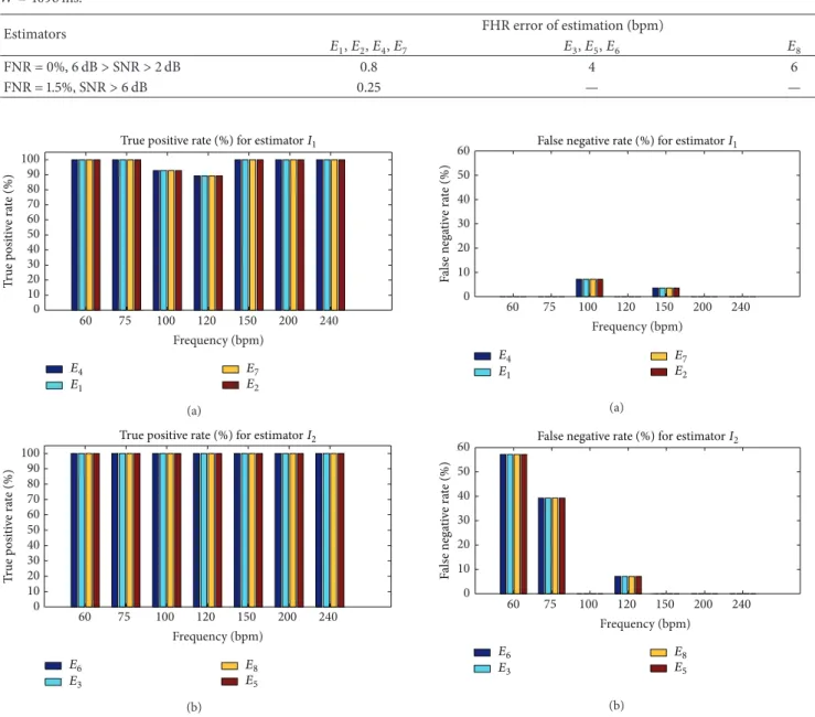
3.1.2. Performance Levels of Estimators. In this study, the performance levels of estimators we wanted to compute were sensitivity and the false negative rate. Fetal heart rates
were evaluated every 250 ms from noisy signals with𝑊 =
4096 ms. Sensitivity was computed with the equation: 𝑆 = TP/(TP + FN), where TP was the true positive rate and FN was the false negative rate. Estimates of simulated heart rate were considered to be false negative if they did not ensure the expected accuracy; otherwise, they were true positive. Sensitivity and the false positive rate were evaluated as the
Table 2: FHR error of estimation (bpm) obtained by all estimators tested for different configurations of SNR, false negative rate (FNR), and 𝑊 = 4096 ms.
Estimators FHR error of estimation (bpm)
𝐸1,𝐸2,𝐸4,𝐸7 𝐸3,𝐸5,𝐸6 𝐸8 FNR = 0%, 6 dB> SNR > 2 dB 0.8 4 6 FNR = 1.5%, SNR> 6 dB 0.25 — — 0 10 20 30 40 50 60 70 80 90 100 60 75 100 120 150 200 240 Frequency (bpm) E4 E1 E7 E2
True positive rate (%) for estimator I1
T ru e p o si ti ve r at e ( % ) (a) 0 10 20 30 40 50 60 70 80 90 100 60 75 100 120 150 200 240 Frequency (bpm) E6 E3 E8 E5
True positive rate (%) for estimator I2
T ru e p o si ti ve r at e ( % ) (b)
Figure 6: True positive rates for𝐼1and𝐼2with SNR> 0.6 dB, W = 4096, and an error of estimation of 0.25 bpm. (a) True positive rate for𝐼1. (b) True positive rate for𝐼2.
average of 30 values. Each value was determined after analysis of a noisy signal of 30 s where sensitivity and the false positive rate had converged to the highest value and to the lowest value, respectively. Convergence was reached for a minimum SNR of 6 dB.
The results of this second series of simulations are
presented in Figures 6 and 7 for𝑊 = 4096 ms and SNR ≥
6 dB. Note that the estimation of error of 25 bpm was obtained only for𝐼1whatever the frequency, whereas accuracy for𝐼2 was obtained only for 100, 150, 200, 220, and 240 bpm.
The results set out in Figure 7 show that estimators based on𝐼1(𝐸1,𝐸2,𝐸4, and𝐸7) had an average (average obtained from the cardiac frequency) false negative rate of 1.5%, while those based on 𝐼2 (𝐸3, 𝐸5, 𝐸6, and𝐸8) presented a higher
0 10 20 30 40 50 60 60 75 100 120 150 200 240 Frequency (bpm) E4 E1 E7 E2 False negative rate (%) for estimator I1
F als e nega ti ve ra te ( % ) (a) 0 10 20 30 40 50 60 60 75 100 120 150 200 240 Frequency (bpm) E6 E3 E8 E5
False negative rate (%) for estimator I2
F als e nega ti ve ra te ( % ) (b)
Figure 7: False negative rates for 𝐼1 and𝐼2 with SNR> 0.6 dB, W = 4096. Accuracy of 25 bpm was obtained only for𝐼1whatever the frequency, whereas for𝐼2accuracy was obtained for only 100, 150, 200, 220, and 240 bpm. (a) False negative rate for𝐼1. (b) False negative rate for𝐼2.
average false negative rate of approximately 14.8%. The 97.5% average true positive rate of𝐼1 was slightly lower than that of estimators based on𝐼2, which was 100%. Finally, when the accuracy of 0.25 bpm was reached, we observed that the estimators based on 𝐼1 were generally more accurate than those based on𝐼2, although the average false negative rate was not zero.
Figure 8 shows the error of estimation corresponding to different values of SNR when a zero false negative rate was imposed. This zero false negative rate was obtained by modifying the detection threshold, and a direct consequence was an increase in the estimation. The results derived from Figure 8 showed that the zero false negative rate for𝐼1 was
Table 3: Sensitivity (%) of estimators for 𝑊 = 4096 ms. 𝐼1 and 𝐼2 are the two autocorrelation estimators, respectively.𝑥𝐵,𝑥𝐹are
the envelopes of directional signals, and𝑥𝑒is the envelope of the nondirectional signal.𝐹𝑢𝑠 indicates the combined estimator.
Sensitivity (𝑆) Estimators 𝐼1 𝐼2 𝑆(𝑥𝐵) 88.50% (𝐸4) 88.43% (𝐸6) 𝑆(𝑥𝐹) 86.63% (𝐸1) 84.79% (𝐸3) 𝑆(𝑥𝑒) 81.79% (𝐸7) 75.05% (𝐸8) 𝑆(𝐹𝑢𝑠) 95.48% (𝐸2) 94.93% (𝐸5)
ensured for a SNR ≥ 2 dB (below the SNR measured on
real signals) and for an error of estimation of 0.8 bpm. In the case of𝐼2 and directional signals, we obtained an error of estimation of 4 bpm, whereas for a nondirectional signal it was 6 bpm.
Table 2 summarizes the effectiveness of each estimator in terms of FHR error of estimation, SNR, and average false negative rate. To reach an error of estimation, that is, the expected accuracy of 0.25 bpm, we recommend 𝐼1, that is, autocorrelation-based estimators (𝐸1, 𝐸2, 𝐸4, and𝐸7), the price to be paid being an average false negative rate of 1.5%. To reach an average false negative rate of 0%, we recommend𝐼1 autocorrelation-based estimators (𝐸1,𝐸2,𝐸4, and𝐸7), where the price to be paid is an error of estimation of 0.8 bpm far from the expected accuracy of 0.25 bpm.
3.2. Results Obtained on Real Signals. We recorded 580 minutes for the analysis of real Doppler signals. We selected areas where signals had the cardiac activity signature. The performance levels on these signals were evaluated on the envelopes of both the nondirectional and the directional signals. The FHR estimation obtained with a commercial device (Oxford Sonicaid) was used as a reference to evaluate sensitivity which was evaluated for each estimator. All esti-mators were evaluated using a size of𝑊 = 4096 ms.
The results obtained for all the signals are presented in Table 3. The estimators based on directional signals (𝐸1,𝐸4, 𝐸3, and𝐸6) provided a higher level of sensitivity compared
to those which used nondirectional signals (𝐸7,𝐸8). In the case of directional signals, the results of𝐼1and𝐼2were close but slightly better for 𝐼1. This result confirmed the results obtained by simulations. We therefore recommend the use of estimators based on𝐼1 calculated on the directional signals (𝐸1,𝐸4).
Sensitivity was improved using the combination method. The sensitivity of estimator𝐸2was 95.5% (see Table 3). Using the combination method, the sensitivity increased to about (95.5%–88.5%)≈ 7% compared to directional signals 𝐸4and
to about (95.5%–81.8%)≈ 14% compared to nondirectional
signals𝐸7.
4. Discussion and Conclusion
In this study, we focused on different settings of the estimators (window size, lag) that ensured a fetal heart rate estimation
0 5 10 15 20 Directional signal FHR er ro r o f es ti m at io n ( b p m) 0.0 0.2 0.4 0.6 0.8 1.0 1.2 1.4 1.6 1.8 2.0 SNR (dB) Estimator I1 Estimator I2 0.25 bpm (a) 0 5 10 15 20 FHR er ro r o f es ti m at io n ( b p m) Nondirectional signal 0.0 0.2 0.4 0.6 0.8 1.0 1.2 1.4 1.6 1.8 2.0 SNR (dB) Estimator I1 Estimator I2 0.25 bpm (b) 0 5 10 15
20 Combined estimators of directional signal
FHR er ro r o f es ti m at io n ( b p m) 0.0 0.2 0.4 0.6 0.8 1.0 1.2 1.4 1.6 1.8 2.0 SNR (dB) Estimator I1 Estimator I2 0.25 bpm 0.8 b p m (c)
Figure 8: FHR error of estimation (bpm) when the false negative rate was zero, when the SNR ∈ (0 dB, 2 dB), and when the signals tested were𝑥𝐹,𝑥𝐵, and𝑥𝑒.
with a maximum authorized error of 0.25 bpm. We found in simulation that only estimators based on𝐼1and directional signals could ensure such an accuracy of 0.25 bpm. The size necessary in this case was𝑊 = 4096 ms.
Note that, although we proposed synthetic signals that were as realistic as possible, we are aware that the plotted performance levels are representative only of our simulations and not of all cases encountered in practice. It is likely that the performance levels of the algorithms tested can be reduced in the presence of artefacts. However, the 95% sensitivity obtained from real signals suggests that our proposed esti-mators may be trusted.
In the case of real signals, the sensitivity was quantified. Since in our study the estimated SNR on the real signals was greater than the threshold of 6 dB (deduced on simulated signals) required to reach the desired accuracy of 0.25 bpm, a denoising filter was not necessary. However, in cases of a
SNR lower than 6 dB, a denoising process (Wiener, wavelet) could be introduced.
Sensitivity was quantified using a 𝑊 size of 4096 ms. We found that the estimators 𝐸1, 𝐸2, and𝐸4 based on 𝐼1 had slightly greater sensitivity than those based on 𝐼2. We therefore recommend the use of𝐼1.
Various cases were considered on the basis of this study, that is, those that do not require a precise estimate of the fetal heart rate and those for which accuracy is critical. The accuracy of fetal heart rate estimation in the first case is not important but the false negative rate should be as low as possible. For example, if the goal of a monitoring system is simply to verify that the fetal heart rate is in the normal range (110–160 bpm), very high accuracy is not needed. In this case, an error of estimation of 0.8 bpm is sufficient. Our computations showed that for an error of estimation of 0.8 bpm, a zero false negative rate in the zones when the rhythm is quasi-constant could be ensured. In the second case, an error of estimation of 0.25 bpm is required for a system in which the goal is not only to estimate the heart rate, but also to evaluate fetal wellbeing. Our study showed that for this type of system, the false negative rate may be slightly higher than zero. It is important to note that this error of estimation was guaranteed for a quasi-constant heart rate. This is not a constraint for such a system, since the variability of fetal heart rate must be evaluated in these ranges to predict fetal distress.
Applied to real signals, the estimators based on 𝐼1 pro-vided sensitivity close to those of𝐼2, and the most efficient of these estimators were those that used directional signals (𝐸1, 𝐸2, and𝐸4).
A 7% increase in sensitivity compared to estimators based on individual directional signals was possible when we combined the two heart rates calculated on the directional signals. A 14% increase in sensitivity compared to estimators based on individual nondirectional signals was possible when we combined the two heart rates calculated on the directional signals. When a combination was used, both signals were processed in parallel, thus doubling the number of operations.
The good levels of performance of our estimator based on this combination suggest first that it can be adapted to multitransducer, multichannel configurations and second that such an estimator will improve fetal diagnosis.
Conflict of Interests
The authors declare that there is no conflict of interests regarding the publication of this paper.
Acknowledgments
This study was supported by the Agence Nationale de la Research (Project ANR-07-TECSAN-023, Surfoetus). The authors would like to thank the Clinical Investigation Centre for Innovative Technology of Tours (CIC-IT 806 CHRU of Tours) and Professor F. Perrotin’s Obstetric Department Team for their support in recording the signals. The authors
would like to thank the anonymous referees for their valuable comments.
References
[1] F. Manning, I. Morrison, I. Lange, C. Harman, and P. Chamber-lain, “Fetal assessment based on fetal biophysical profile scoring: experience in 12, 620 referred high-risk pregnancies. I. Perinatal mortality by frequency and etiology,” The American Journal of Obstetrics and Gynecology, vol. 151, no. 3, pp. 343–350, 1985. [2] H.-Y. Chen, S. P. Chauhan, C. V. Ananth, A. M. Vintzileos, and
A. Z. Abuhamad, “Electronic fetal heart rate monitoring and infant mortality: a population-based study in the United States,” The American Journal of Obstetrics and Gynecology, vol. 204, no. 6, pp. S43–S44, 2011.
[3] G. G. Berntson, J. Thomas Bigger Jr., D. L. Eckberg et al., “Heart rate variability: origins methods, and interpretive caveats,” Psychophysiology, vol. 34, no. 6, pp. 623–648, 1997.
[4] M. Malik and A. J. Camm, “Heart rate variability,” Clinical Cardiology, vol. 13, no. 8, pp. 570–576, 1990.
[5] M. David, M. Hirsch, J. Karin, E. Toledo, and S. Akselrod, “An estimate of fetal autonomic state by time-frequency analysis of fetal heart rate variability,” Journal of Applied Physiology, vol. 102, no. 3, pp. 1057–1064, 2007.
[6] B. Arabin and S. Riedewald, “An attempt to quantify character-istics of behavioral states,” The American Journal of Perinatology, vol. 9, no. 2, pp. 115–119, 1992.
[7] B. Frank, B. Pompe, U. Schneider, and D. Hoyer, “Permutation entropy improves fetal behavioural state classification based on heart rate analysis from biomagnetic recordings in near term fetuses,” Medical and Biological Engineering and Computing, vol. 44, no. 3, pp. 179–187, 2006.
[8] S. Lange, P. Van Leeuwen, U. Schneider et al., “Heart rate features in fetal behavioural states,” Early Human Development, vol. 85, no. 2, pp. 131–135, 2009.
[9] J. A. DiPietro, D. M. Hodgson, K. A. Costigan, S. C. Hilton, and T. R. B. Johnson, “Fetal neurobehavioral development,” Child Development, vol. 67, no. 5, pp. 2553–2567, 1996.
[10] M. Ferrario, M. G. Signorini, G. Magenes, and S. Cerutti, “Com-parison of entropy-based regularity estimators: application to the fetal heart rate signal for the identification of fetal distress,” IEEE Transactions on Biomedical Engineering, vol. 53, no. 1, pp. 119–125, 2006.
[11] A. Kikuchi, T. Shimizu, A. Hayashi et al., “Nonlinear analyses of heart rate variability in normal and growth-restricted fetuses,” Early Human Development, vol. 82, no. 4, pp. 217–226, 2006. [12] G. S. Dawes, M. O. Lobbs, G. Mandruzzato, M. Moulden, C. W.
G. Redman, and T. Wheeler, “Large fetal heart rate decelerations at term associated with changes in fetal heart rate variation,” The American Journal of Obstetrics and Gynecology, vol. 188, no. 1, pp. 105–111, 1993.
[13] J. Jezewski, J. Wrobel, and K. Horoba, “Comparison of Doppler ultrasound and direct electrocardiography acquisition tech-niques for quantification of fetal heart rate variability,” IEEE Transactions on Biomedical Engineering, vol. 53, no. 5, pp. 855– 864, 2006.
[14] J. Pardey, M. Moulden, and C. W. G. Redman, “A computer system for the numerical analysis of nonstress tests,” The American Journal of Obstetrics and Gynecology, vol. 186, no. 5, pp. 1095–1103, 2002.
[15] E. Courtin, W. Ruchay, P. Salfeld, H. Sommer, and A. Versatile, “Semiautomatic fetal monitor for non-technical users,” Hewlett-Packard Journal, vol. 28, no. 5, pp. 16–23, 1977.
[16] T. Kret and K. Kaluzynski, “The fetal heart rate estimation based on continuous ultrasonic Doppler data,” Biocybernetics and Biomedical Engineering, vol. 26, no. 3, pp. 49–56, 2006. [17] I. Voicu, D. Kouame, M. Fournier-Massignan, and J.-M. Girault,
“Estimating fetal heart rate from multiple ultrasound signals,” in Proceedings of the International Conference on Advancements of Medicine and Health Care through Technology, pp. 185–190, Berlin, Germany, September 2009.
[18] A. Krib`eche, F. Tranquart, D. Kouame, and L. Pourcelot, “The Actifetus system: a multidoppler sensor system for monitoring fetal movements,” Ultrasound in Medicine and Biology, vol. 33, no. 3, pp. 430–438, 2007.
[19] J. A. Jensen, Estimation of Blood Velocities Using Ultrasound, Cambridge University Press, Cambridge, UK, 1996.
[20] N. Aydin, L. Fan, and D. H. Evans, “Quadrature-to-directional format conversion of Doppler signals using digital methods,” Physiological Measurement, vol. 15, no. 2, article 007, pp. 181–199, 1994.
[21] S. A. Shakespeare, J. A. Crowe, B. R. Hayes-Gill, K. Bhogal, and D. K. James, “The information content of Doppler ultrasound signals from the fetal heart,” Medical and Biological Engineering and Computing, vol. 39, no. 6, pp. 619–626, 2001.
[22] E. Hernandez-Andrade, H. Figueroa-Diesel, C. Kottman et al., “Gestational-age-adjusted reference values for the modified myocardial performance index for evaluation of fetal left cardiac function,” Ultrasound in Obstetrics and Gynecology, vol. 29, no. 3, pp. 321–325, 2007.
[23] A. V. Oppenheim and R. W. Schafer, Discrete-Time Signal Proc-essing, Prentice Hall Signal ProcProc-essing, Prentice-Hall Interna-tional, Englewood Cliffs, NJ, USA, 1989.