Converse results on existence of
sum of squares Lyapunov functions
The MIT Faculty has made this article openly available.
Please share
how this access benefits you. Your story matters.
Citation
Ahmadi, Amir Ali, and Pablo A. Parrilo. “Converse Results on
Existence of Sum of Squares Lyapunov Functions.” 50th IEEE
Conference on Decision and Control and European Control
Conference 2011 (CDC-ECC). 6516–6521.
As Published
http://dx.doi.org/10.1109/CDC.2011.6161493
Publisher
Institute of Electrical and Electronics Engineers (IEEE)
Version
Author's final manuscript
Citable link
http://hdl.handle.net/1721.1/72483
Terms of Use
Creative Commons Attribution-Noncommercial-Share Alike 3.0
Converse Results on Existence of Sum of Squares Lyapunov Functions
Amir Ali Ahmadi and Pablo A. Parrilo
Abstract— Despite the pervasiveness of sum of squares (sos) techniques in Lyapunov analysis of dynamical systems, the converse question of whether sos Lyapunov functions exist whenever polynomial Lyapunov functions exist has remained elusive. In this paper, we first show via an explicit counterex-ample that if the degree of the polynomial Lyapunov function is fixed, then sos programming can fail to find a valid Lyapunov function even though one exists. On the other hand, if the degree is allowed to increase, we prove that existence of a polynomial Lyapunov function for a homogeneous polynomial vector field implies existence of a polynomial Lyapunov function that is sos and that the negative of its derivative is also sos. The latter result is extended to develop a converse sos Lyapunov theorem for robust stability of switched linear systems.
I. INTRODUCTION
Consider a continuous time dynamical system ˙
x = f (x), (1) where f : Rn → Rn is a polynomial and has an equilibrium
at the origin, i.e., f (0) = 0. When a polynomial function V (x) : Rn → R is used as a candidate Lyapunov function
for stability analysis of system (1), conditions of Lyapunov’s theorem reduce to a set of polynomial inequalities. For instance, if establishing global asymptotic stability of the origin is desired, one would require a radially unbounded polynomial Lyapunov candidate to vanish at the origin and satisfy
V (x) > 0 ∀x 6= 0 (2) ˙
V (x) = h∇V (x), f (x)i < 0 ∀x 6= 0. (3) Here, ˙V denotes the time derivative of V along the trajecto-ries of (1), ∇V (x) is the gradient vector of V , and h., .i is the standard inner product in Rn. In some other variants of the
analysis problem, e.g. if LaSalle’s invariance principle is to be used, or if the goal is to prove boundedness of trajectories of (1), then the inequality in (3) is replaced with
˙
V (x) ≤ 0 ∀x. (4) In any case, the problem arising from this analysis approach is that even though polynomials of a given degree are finitely parameterized, the computational problem of searching for a polynomial V satisfying inequalities of the type (2),(3),(4) is intractable. In fact, even deciding if a given polynomial V of degree four or larger satisfies (2) is NP-hard [1].
An approach pioneered in [2] and widely popular by now is to replace the positivity (or nonnegativity) conditions by
Amir Ali Ahmadi and Pablo A. Parrilo are with the Laboratory for Information and Decision Systems, Department of Electrical Engineering and Computer Science, Massachusetts Institute of Technology. E-mail: a a a@mit.edu, parrilo@mit.edu.
the requirement of the existence of a sum of squares (sos) decomposition:
V sos (5)
− ˙V = −h∇V, f i sos. (6) Clearly, if a polynomial is a sum of squares, then it is nonnegative. Moreover, because of some interesting con-nections between real algebra and convex optimization, it turns out that the existence of an sos decomposition can be cast as the feasibility of a semidefinite program (SDP) [3], which can be solved efficiently e.g. by using interior point algorithms [4]. We call a Lyapunov function satisfying both sos conditions in (5) and (6) a sum of squares Lyapunov function. We emphasize that this is the sensible definition of a sum of squares Lyapunov function and not what the name may suggest, which is a Lyapunov function that is a sum of squares. Indeed, the underlying semidefinite program will find a Lyapunov function V if and only if V satisfies both conditions (5) and (6).
Over the last decade, the applicability of sum of squares Lyapunov functions has been explored and extended in many directions and a multitude of sos techniques have been developed to tackle a range of problems in systems and control. We refer the reader to the by no means exhaustive list of works [5], [6], [7], [8], [9], [10], [11], [12], [13], and references therein. Despite the wealth of research in this area, the converse question of whether the existence of a polynomial Lyapunov function implies the existence of a sum of squares Lyapunov function has remained unresolved. This question naturally comes in two variants:
Problem 1: Does existence of a polynomial Lyapunov function of a given degree imply existence of a polynomial Lyapunov function of the same degree that satisfies the sos conditions in (5) and (6)?
Problem 2: Does existence of a polynomial Lyapunov function of a given degree imply existence of a polynomial Lyapunov function of possibly higher degree that satisfies the sos conditions in (5) and (6)?
The main contribution of this paper is to give a negative answer to Problem 1 (Section III) and a positive answer to Problem 2 under an additional homogeneity assumption (Section IV). We stress that these results do not follow a priori from well-known facts about the gap between nonneg-ative and sum of squares polynomials because of the distinct features involved in the problem of a search for Lyapunov functions; see e.g. Remark 2.1 in Section II.
In all the problems that we consider in this paper, the notion of stability of interest is global asymptotic stability.
Of course, a fundamental question that comes before the problems mentioned above is the following:
Problem 0: If a polynomial dynamical system is globally asymptotically stable, does it admit a polynomial Lyapunov function?
In joint work with Miroslav Krstic, we have recently answered this question in the negative via an explicit coun-terexample [14]. This, however, is not the focus of the current paper.
A. Related literature
Closely related to this paper are the works in [15] and [16]. In previous work [17], Peet proves that exponentially stable polynomial systems have polynomial Lyapunov functions on bounded regions. In [15], [16], Peet and Papachristodoulou extend this result to show that the Lyapunov function can be taken to be a sum of squares if the degree is allowed to increase. A bound on the degree of this Lyapunov function is also provided in [16]. The proof technique used in [15], [16], is based on approximating the solution map using the Picard iteration and is interesting in itself, though the actual conclusion that a Lyapunov function that is sos exists has a far simpler proof: If a polynomial function V is a Lyapunov function for system (1), then so is V2 which is clearly a
sum of squares; see Lemma 4.1 in Section IV. Furthermore, the results in [15], [16] do not lead to any conclusions as to whether the negative of the derivative of the Lyapunov function is sos, i.e, whether condition (6) is satisfied. As we remarked before, there is therefore no guarantee that the semidefinite program can find such a Lyapunov function. (See our counterexample in Section III where this very phenomenon occurs.)
Other related work in the control literature include the work of Chesi in [18] where the gap between positive and sos polynomials is studied, and the work of Peyrl and Parrilo in [19] where it is shown that certificates of infeasibility of the sos Lyapunov problem in (5), (6) can be extracted from equilibria, orbits, or unbounded solutions. Parts of the results of the current paper have appeared in the Master’s thesis of the first author [20].
B. Organization of this paper
The organization of this paper is as follows. In Section II, we recall a few basic definitions and review some known results on the gap between nonnegative and sum of squares polynomials. We also give a motivating example of a stable vector field for which no polynomial Lyapunov function of degree less than 8 exists (Example 2.1). In Section III, we prove via an explicit counterexample that if the degree of the Lyapunov function is fixed, then the sos Lyapunov require-ments are strictly more conservative than the requirement of existence of a polynomial Lyapunov function. In Section IV, we show that for a homogeneous vector field existence of a polynomial Lyapunov function implies existence of a polynomial Lyapunov function (of possibly higher degree) that is sos and that the negative of its derivative is also sos (Theorem 4.3). The proof of this theorem is quite simple
and relies on a powerful recent Positivstellensatz result due to Scheiderer (Theorem 4.2). In Section IV-A, we extend these results to the problem of robust analysis of switched linear systems and prove that if such a system is stable under arbitrary switching, then it admits a common sos polynomial Lyapunov function whose derivative also satisfies the sos condition (Theorem 4.4). We present a summary of the paper and some future directions and open problems in Section V.
II. PRELIMINARIES
Throughout the paper, we will be concerned with Lya-punov functions that are (multivariate) polynomials. We say that a Lyapunov function V is nonnegative if V (x) ≥ 0 for all x ∈ Rn, and that it is positive definite if V (x) > 0 for
all x ∈ Rn\{0} and V (x) = 0. Clearly, for a polynomial
to be nonnegative its degree should be even. A polynomial V of degree d is said to be homogeneous if it satisfies V (λx) = λd
V (x) for any scalar λ ∈ R. This condition holds if and only if all monomials of V have degree d. It is easy to see that homogeneous polynomials are closed under sums and products and that the gradient of a homogeneous polynomial has entries that are homogeneous polynomials.
We say that a polynomial V is a sum of squares (sos) if V =Pm
i q 2
i for some polynomials qi. We do not present here
the semidefinite program that decides if a given polynomial is sos since it has already appeared in several places. The unfamiliar reader is referred to [3]. If V is sos, then V is nonnegative. Moreover, when an sos feasibility problem is strictly feasible, the polynomials returned by interior point algorithms are positive definite; see [20, p. 41]. Because of this fact, we impose the sos Lyapunov conditions in (5) and (6) as sufficient conditions for the inequalities in (2) and (3). In 1888, Hilbert [21] showed that for polynomials in n variables and of degree d, the notions of nonnegativity and sum of squares are equivalent if and only if n = 1, d = 2, or (n, d)=(2, 4). A homogeneous version of the same result states that nonnegative homogeneous polynomials in n variables and of degree d are sums of squares if and only if n = 2, d = 2, or (n, d)=(3, 4). The first explicit example of a nonnegative polynomial that is not sos is due to Motzkin [22] and appeared nearly 80 years after the paper of Hilbert; see the survey in [23]. Still today, finding examples of such polynomials is a challenging task, especially if additional structure is required on the polynomial; see e.g. [24]. This itself is a premise for the powerfulness of sos techniques at least in low dimensions and degrees.
Remark 2.1: Existence of nonnegative polynomials that are not sums of squares does not imply on its own that the sos conditions in (5) and (6) are more conservative than the Lyapunov inequalities in (2) and (3). Since Lyapunov functions are not in general unique, it could happen that within the set of valid polynomial Lyapunov functions of a given degree, there is always at least one that satisfies the sos conditions (5) and (6). Moreover, many of the known examples of nonnegative polynomials that are not sos have multiple zeros and local minima [23] and therefore cannot serve as Lyapunov functions. Indeed, if a function has a local
minimum other than the origin, then its value evaluated on a trajectory starting from the local minimum would not be decreasing.
A. A motivating example
The following example will help motivate the kind of questions that we are addressing in this paper.
Example 2.1: Consider the dynamical system ˙ x1 = −0.15x71+ 200x61x2− 10.5x51x22− 807x41x32 +14x3 1x42+ 600x21x25− 3.5x1x62+ 9x72 ˙ x2 = −9x71− 3.5x61x2− 600x51x22+ 14x41x32 +807x3 1x42− 10.5x21x25− 200x1x62− 0.15x72. (7) A typical trajectory of the system that starts from the initial condition x0 = (2, 2)T is plotted in Figure 1. Our goal
is to establish global asymptotic stability of the origin by searching for a polynomial Lyapunov function. Since the vector field is homogeneous, the search can be restricted to homogeneous Lyapunov functions [25]. To employ the sos technique, we can use the software package SOSTOOLS [26] to search for a Lyapunov function satisfying the sos condi-tions (5) and (6). However, if we do this, we will not find any Lyapunov functions of degree 2, 4, or 6. If needed, a certificate from the dual semidefinite program can be obtained, which would prove that no polynomial of degree up to 6 can satisfy the sos requirements (5) and (6).
At this point we are faced with the following question. Does the system really not admit a Lyapunov function of degree 6 that satisfies the true Lyapunov inequalities in (2), (3)? Or is the failure due to the fact that the sos conditions in (5), (6) are more conservative?
Note that when searching for a degree 6 Lyapunov func-tion, the sos constraint in (5) is requiring a homogeneous polynomial in 2 variables and of degree 6 to be a sum of squares. The sos condition (6) on the derivative is also a condition on a homogeneous polynomial in 2 variables, but in this case of degree 12. (This is easy to see from ˙V = h∇V, f i.) By the results of the previous subsection, we know that nonnegativity and sum of squares are equivalent notions for homogeneous bivariate polynomials, irrespective of the degree. Hence, we now have a proof that this dynamical system truly does not have a Lyapunov function of degree 6 (or lower).
This fact is perhaps geometrically intuitive. Figure 1 shows that the trajectory of this system is stretching out in 8 different directions. So, we would expect the degree of the Lyapunov function to be at least 8. Indeed, when we increase the degree of the candidate function to 8, SOSTOOLS and the SDP solver SeDuMi [27] succeed in finding the following Lyapunov function: V (x) = 0.02x81+ 0.015x71x2+ 1.743x61x 2 2− 0.106x 5 1x 3 2 −3.517x4 1x 4 2+ 0.106x 3 1x 5 2+ 1.743x 2 1x 6 2 −0.015x1x72+ 0.02x 8 2.
The level sets of this Lyapunov function are plotted in Figure 1 and are clearly invariant under the trajectory.
Fig. 1. A typical trajectory of the vector filed in Example 2.1 (solid), level sets of a degree 8 polynomial Lyapunov function (dotted).
III. ACOUNTEREXAMPLE
Unlike the scenario in the previous example, we now show that a failure in finding a Lyapunov function of a particular degree via sum of squares programming can also be due to the gap between nonnegativity and sum of squares. What will be conservative in the following counterexample is the sos condition on the derivative.
Consider the dynamical system ˙ x1 = −x31x22+ 2x31x2− x31+ 4x21x22− 8x21x2+ 4x21 −x1x42+ 4x1x32− 4x1+ 10x22 ˙ x2 = −9x21x2+ 10x21+ 2x1x32− 8x1x22− 4x1− x32 +4x2 2− 4x2. (8) One can verify that the origin is the only equilibrium point for this system, and therefore it makes sense to investigate global asymptotic stability. If we search for a quadratic Lya-punov function for (8) using sos programming, we will not find one. It will turn out that the corresponding semidefinite program is infeasible. We will prove shortly why this is the case, i.e, why no quadratic function V can satisfy
V sos
− ˙V sos. (9) Nevertheless, we claim that
V (x) = 1 2x 2 1+ 1 2x 2 2 (10)
is a valid Lyapunov function. Indeed, one can check that ˙
V (x) = x1x˙1+ x2x˙2= −M (x1− 1, x2− 1), (11)
where M (x1, x2) is the Motzkin polynomial [22]:
M (x1, x2) = x41x 2 2+ x 2 1x 4 2− 3x 2 1x 2 2+ 1.
This polynomial is known to be nonnegative but not sos. (Nonnegativity follows easily from the arithmetic-geometric inequality; for a proof that M is not sos see [23].) The polynomial ˙V is strictly negative everywhere, except for the origin and three other points (0, 2)T, (2, 0)T, and (2, 2)T,
where ˙V is zero. However, at each of these three points we have ˙x 6= 0. Once the trajectory reaches any of these three points, it will be kicked out to a region where ˙V is strictly negative. Therefore, by LaSalle’s invariance principle (see e.g. [28, p. 128]), the quadratic Lyapunov function in (10) proves global asymptotic stability of the origin of (8).
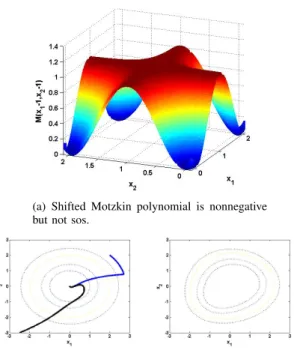
(a) Shifted Motzkin polynomial is nonnegative but not sos.
(b) Typical trajectories of (8) (solid), level sets of V (dotted).
(c) Level sets of a quartic Lya-punov function found through sos programming.
Fig. 2. The quadratic polynomial12x2 1+
1 2x
2
2is a valid Lyapunov function for the vector field in (8) but it is not detected through sos programming.
The fact that ˙V is zero at three points other than the origin is not the reason why sos programming is failing. After all, when we impose the condition that − ˙V should be sos, we allow for the possibility of a non-strict inequality. The reason why our sos program does not recognize (10) as a Lyapunov function is that the shifted Motzkin polynomial in (11) is nonnegative but it is not a sum of squares. This sextic polynomial is plotted in Figure 2(a). Trajectories of (8) starting at (2, 2)T and (−2.5, −3)T along with level sets of V are shown in Figure 2(b).
So far, we have shown that V in (10) is a valid Lyapunov function but does not satisfy the sos conditions in (9). We still need to show why no other quadratic Lyapunov function U (x) = c1x21+ c2x1x1+ c3x22 (12)
can satisfy the sos conditions either.1 We will in fact prove
the stronger statement that V in (10) is the only valid quadratic Lyapunov function for this system up to scaling, i.e., any quadratic function U that is not a scalar multiple of 12x21+12x
2
2 cannot satisfy U ≥ 0 and − ˙U ≥ 0. It will
even be the case that no such U can satisfy − ˙U ≥ 0 alone. (The latter fact is to be expected since global asymptotic stability of (8) together with − ˙U ≥ 0 would automatically imply U ≥ 0; see [29, Theorem 1.1].)
So, let us show that − ˙U ≥ 0 implies U is a scalar multiple of 12x2
1+12x 2
2. Because Lyapunov functions are closed under
positive scalings, without loss of generality we can take
1Since the Lyapunov function U and its gradient have to vanish at the origin, linear or constant terms are not needed in (12).
c1 = 1. One can check that
− ˙U (0, 2) = −80c2,
so to have − ˙U ≥ 0, we need c2≤ 0. Similarly,
− ˙U (2, 2) = −288c1+ 288c3,
which implies that c3≥ 1. Let us now look at
− ˙U (x1, 1) = −c2x31+ 10c2x21+ 2c2x1− 10c2− 2c3x21
+20c3x1+ 2c3+ 2x21− 20x1.
(13) If we let x1 → −∞, the term −c2x31 dominates this
polynomial. Since c2 ≤ 0 and − ˙U ≥ 0, we conclude that
c2 = 0. Once c2 is set to zero in (13), the dominating
term for x1 large will be (2 − 2c3)x21. Therefore to have
− ˙U (x1, 1) ≥ 0 as x1→ ±∞ we must have c3≤ 1. Hence,
we conclude that c1 = 1, c2 = 0, c3 = 1, and this finishes
the proof.
Even though sos programming failed to prove stability of the system in (8) with a quadratic Lyapunov function, if we increase the degree of the candidate Lyapunov function from 2 to 4, then SOSTOOLS succeeds in finding a quartic Lyapunov function W (x) = 0.08x41− 0.04x 3 1+ 0.13x 2 1x 2 2+ 0.03x 2 1x2 +0.13x21+ 0.04x1x22− 0.15x1x2 +0.07x42− 0.01x32+ 0.12x 2 2,
which satisfies the sos conditions in (9). The level sets of this function are close to circles and are plotted in Figure 2(c).
Motivated by this example, it is natural to ask whether it is always the case that upon increasing the degree of the Lyapunov function one will find Lyapunov functions that satisfy the sum of squares conditions in (9). In the next section, we will prove that this statement is indeed true at least for homogeneous vector fields.
IV. ACONVERSESOS LYAPUNOV THEOREM
We start by noting that existence of a polynomial Lya-punov function trivially implies existence of a LyaLya-punov function that is a sum of squares.
Lemma 4.1: If a polynomial dynamical system has a positive definite polynomial Lyapunov function V with a negative definite derivative ˙V , then it also admits a positive definite polynomial Lyapunov function W which is a sum of squares.
Proof: Take W = V2. The negative of the derivative − ˙W = −2V ˙V is clearly positive definite (though it may not be sos).
We will next prove a result that guarantees the derivative of the Lyapunov function will also satisfy the sos condition, though this result is restricted to homogeneous systems.
A polynomial vector field ˙x = f (x) is homogeneous if all entries of f are homogeneous polynomials of the same degree, i.e., if all the monomials in all the entries of f have the same degree. (For example, the vector field in (7) is homogeneous of degree 7.) Homogeneous systems are extensively studied in the literature on nonlinear control; see
e.g. [30], [25], [31] and references therein.2 A basic fact about homogeneous vector fields is that for these systems the notions of local and global stability are equivalent. Indeed, a homogeneous vector field of degree d satisfies f (λx) = λdf (x) for any scalar λ, and therefore the value of f on the
unit sphere determines its value everywhere. It is also well-known that an asymptotically stable homogeneous system admits a homogeneous Lyapunov funciton [25].
We will use the following Positivstellensatz result due to Scheiderer to prove our converse sos Lyapunov theorem.
Theorem 4.2 (Scheiderer, [32]): Given any two positive definite homogeneous polynomials p and q, there exists an integer k such that pqk is a sum of squares.
Theorem 4.3: Given a homogeneous polynomial vector field, suppose there exists a homogeneous polynomial Lya-punov function V such that V and − ˙V are positive definite. Then, there also exists a homogeneous polynomial Lyapunov function W such that W is sos and − ˙W is sos.
Proof: Observe that V2 and −2V ˙V are both positive
definite and homogeneous polynomials. Applying Theo-rem 4.2 to these two polynomials, we conclude the existence of an integer k such that (−2V ˙V )(V2)k is sos. Let
W = V2k+2.
Then, W is clearly sos since it is a perfect even power. Moreover,
− ˙W = −(2k + 2)V2k+1V = −(k + 1)2V˙ 2kV ˙V is also sos by the previous claim.3
A. Existence of sos Lyapunov functions for switched linear systems
The result of Theorem 4.3 extends in a straightforward manner to Lyapunov analysis of switched systems. In par-ticular, we are interested in the highly-studied problem of stability analysis of arbitrary switched linear systems:
˙
x = Aix, i ∈ {1, . . . , m}, (14)
Ai ∈ Rn×n. We assume the minimum dwell time of the
system is bounded away from zero. This guarantees that the solutions of (14) are well-defined. Existence of a common Lyapunov function is necessary and sufficient for (global) asymptotic stability under arbitrary switching (ASUAS) of system (14). The ASUAS of system (14) is equivalent to asymptotic stability of the linear differential inclusion
˙
x ∈ co{Ai}x, i ∈ {1, . . . , m},
where co here denotes the convex hull. It is also known that ASUAS of (14) is equivalent to exponential stability under arbitrary switching [33]. A common approach for analyzing the stability of these systems is to use the sos technique to search for a common polynomial Lyapunov function [9], [11]. We will prove the following result.
2Beware that the definition of a homogeneous vector field in these references is more general than the one we are using here.
3Note that W and − ˙W are positive definite and therefore prove global asymptotic stability.
Theorem 4.4: The switched linear system in (14) is asymptotically stable under arbitrary switching if and only if there exists a common homogeneous polynomial Lyapunov function W such that
W sos − ˙Wi= −h∇W (x), Aixi sos,
for i = 1, . . . , m, where the polynomials W and − ˙Wi are
all positive definite.
To prove this result, we will use the following theorem of Mason et al.
Theorem 4.5 (Mason et al., [34]): If the switched linear system in (14) is asymptotically stable under arbitrary switching, then there exists a common homogeneous poly-nomial Lyapunov function V such that
V > 0 ∀x 6= 0 − ˙Vi(x) = −h∇V (x), Aixi > 0 ∀x 6= 0,
for i = 1, . . . , m.
The next proposition is an extension of Theorem 4.3 to switched systems (not necessarily linear).
Proposition 1: Consider an arbitrary switched dynamical system
˙
x = fi(x), i ∈ {1, . . . , m},
where fi(x) is a homogeneous polynomial vector field of
degree di (the degrees of the different vector fields can be
different). Suppose there exists a common positive definite homogeneous polynomial Lyapunov function V such that
− ˙Vi(x) = −h∇V (x), fi(x)i
is positive definite for all i ∈ {1, . . . , m}. Then there exists a common homogeneous polynomial Lyapunov function W such that W is sos and the polynomials
− ˙Wi= −h∇W (x), fi(x)i,
for all i ∈ {1, . . . , m}, are also sos.
Proof: Observe that for each i, the polynomials V2
and −2V ˙Vi are both positive definite and homogeneous.
Applying Theorem 4.2 m times to these pairs of polynomials, we conclude the existence of positive integers ki such that
(−2V ˙Vi)(V2)ki is sos, (15)
for i = 1, . . . , m. Let
k = max{k1, . . . , km},
and let
W = V2k+2.
Then, W is clearly sos. Moreover, for each i, the polynomial − ˙Wi = −(2k + 2)V2k+1V˙i
= −(k + 1)2V ˙ViV2kiV2(k−ki)
is sos since (−2V ˙Vi)(V2ki) is sos by (15), V2(k−ki) is sos
as an even power, and products of sos polynomials are sos. The proof of Theorem 4.4 now simply follows from Theorem 4.5 and Proposition 1 in the special case where di= 1 for all i.
V. SUMMARY AND FUTURE WORK
We studied the conservatism of the sum of squares relax-ation for establishing stability of polynomial vector fields. We gave a counterexample to show that if the degree of the Lyapunov function is fixed, then the sum of squares conditions on a Lyapunov function and its derivative are more conservative than the true Lyapunov polynomial in-equalities. We then showed that for homogeneous vector fields, existence of a polynomial Lyapunov function implies existence of a Lyapunov function (of possibly higher degree) that satisfies the sos constraints both on the function and on the derivative. We extended this result to show that sum of squares Lyapunov functions are universal for stability of arbitrary switched linear systems.
There are several open questions that one can pursue in the future. We are currently working on proving that stable homogeneous systems admit homogeneous polynomial Lya-punov functions. This combined with Theorem 4.3 would imply that sum of squares Lyapunov functions are necessary and sufficient for proving stability of homogeneous polyno-mial systems. It is not clear to us whether the assumption of homogeneity can be removed from Theorem 4.3. Another research direction would be to obtain upper bounds on the degree of the Lyapunov functions. Some degree bounds are known for Lyapunov analysis of locally exponentially stable systems [16], but they depend on properties of the solution such as convergence rate. Degree bounds on Posi-tivstellensatz result of the type in Theorem 4.2 are typically exponential in size and not very encouraging for practical purposes.
VI. ACKNOWLEDGEMENTS
Amir Ali Ahmadi is thankful to Claus Scheiderer, Greg Blekherman, and Matthew Peet for insightful discussions.
REFERENCES
[1] K. G. Murty and S. N. Kabadi. Some NP-complete problems in quadratic and nonlinear programming. Mathematical Programming, 39:117–129, 1987.
[2] P. A. Parrilo. Structured semidefinite programs and semialgebraic ge-ometry methods in robustness and optimization. PhD thesis, California Institute of Technology, May 2000.
[3] P. A. Parrilo. Semidefinite programming relaxations for semialgebraic problems. Mathematical Programming, 96(2, Ser. B):293–320, 2003. [4] L. Vandenberghe and S. Boyd. Semidefinite programming. SIAM
Review, 38(1):49–95, March 1996.
[5] D. Henrion and A. Garulli, editors. Positive polynomials in control, volume 312 of Lecture Notes in Control and Information Sciences. Springer, 2005.
[6] Special issue on positive polynomials in control. IEEE Trans. Automat. Control, 54(5), 2009.
[7] G. Chesi, A. Garulli, A. Tesi, and A. Vicino. Homogeneous polynomial forms for robustness analysis of uncertain systems. Number 390 in Lecture Notes in Control and Information Sciences. Springer, 2009. [8] Z. Jarvis-Wloszek, R. Feeley, W. Tan, K. Sun, and A. Packard. Some
controls applications of sum of squares programming. In Proceedings of the 42thIEEE Conference on Decision and Control, pages 4676– 4681, 2003.
[9] S. Prajna and A. Papachristodoulou. Analysis of switched and hybrid systems – beyond piecewise quadratic methods. In Proceedings of the American Control Conference, 2003.
[10] S. Prajna, P. A. Parrilo, and A. Rantzer. Nonlinear control synthesis by convex optimization. IEEE Trans. Automat. Control, 49(2):310–314, 2004.
[11] G. Chesi, A. Garulli, A. Tesi, and A. Vicino. Polynomially parameter-dependent Lyapunov functions for robust stability of polytopic sys-tems: an LMI approach. IEEE Trans. Automat. Control, 50(3):365– 370, 2005.
[12] A. A. Ahmadi and P. A. Parrilo. Non-monotonic Lyapunov functions for stability of discrete time nonlinear and switched systems. In Proceedings of the 47thIEEE Conference on Decision and Control, 2008.
[13] E. M. Aylward, P. A. Parrilo, and J. J. E. Slotine. Stability and robustness analysis of nonlinear systems via contraction metrics and SOS programming. Automatica, 44(8):2163–2170, 2008.
[14] A. A. Ahmadi, M. Krstic, and P. A. Parrilo. A globally asymptotically stable polynomial vector field with no polynomial Lyapunov function. 2011. Submitted to the 50th IEEE Conference on Decision and Control.
[15] M. M. Peet and A. Papachristodoulou. A converse sum of squares Lyapunov result: an existence proof based on the Picard iteration. In Proceedings of the 49thIEEE Conference on Decision and Control, 2010.
[16] M. M. Peet and A. Papachristodoulou. A converse sum of squares Lyapunov result with a degree bound. IEEE Trans. Automat. Control, 2011. To appear.
[17] M. M. Peet. Exponentially stable nonlinear systems have polynomial Lyapunov functions on bounded regions. IEEE Trans. Automat. Control, 54(5):979–987, 2009.
[18] G. Chesi. On the gap between positive polynomials and SOS of polynomials. IEEE Trans. Automat. Control, 52(6):1066–1072, 2007. [19] H. Peyrl and P.A. Parrilo. A theorem of the alternative for SOS Lyapunov functions. In Proceedings of the 46th IEEE Conference on Decision and Control, 2007.
[20] A. A. Ahmadi. Non-monotonic Lyapunov functions for stability of nonlinear and switched systems: theory and computation. Master’s Thesis, Massachusetts Institute of Technology, June 2008. Available from http://dspace.mit.edu/handle/1721.1/44206. [21] D. Hilbert. Uber die Darstellung Definiter Formen als Summe von¨
Formenquadraten. Math. Ann., 32, 1888.
[22] T. S. Motzkin. The arithmetic-geometric inequality. In Inequalities (Proc. Sympos. Wright-Patterson Air Force Base, Ohio, 1965), pages 205–224. Academic Press, New York, 1967.
[23] B. Reznick. Some concrete aspects of Hilbert’s 17th problem. In Contemporary Mathematics, volume 253, pages 251–272. American Mathematical Society, 2000.
[24] A. A. Ahmadi and P. A. Parrilo. A convex polynomial that is not sos-convex. Mathematical Programming, 2011. To appear. arXiv:0903.1287.
[25] L. Rosier. Homogeneous Lyapunov function for homogeneous con-tinuous vector fields. Systems Control Lett., 19(6):467–473, 1992. [26] S. Prajna, A. Papachristodoulou, and P. A. Parrilo. SOSTOOLS:
Sum of squares optimization toolbox for MATLAB, 2002-05. Avail-able from http://www.cds.caltech.edu/sostools and http://www.mit.edu/˜parrilo/sostools.
[27] J. Sturm. SeDuMi version 1.05, October 2001. Latest version available at http://sedumi.ie.lehigh.edu/.
[28] H. Khalil. Nonlinear systems. Prentice Hall, 2002. Third edition. [29] A. A. Ahmadi and P. A. Parrilo. On higher order derivatives of
Lyapunov functions. In Proceedings of the 2011 American Control Conference, 2011.
[30] L Gr¨une. Homogeneous state feedback stabilization of homogeneous systems. In Proceedings of the 39thIEEE Conference on Decision and Control, 2000.
[31] L. Moreau, D. Aeyels, J. Peuteman, and R. Sepulchre. Homogeneous systems: stability, boundedness and duality. In Proceedings of the 14th Symposium on Mathematical Theory of Networks and Systems, 2000. [32] C. Scheiderer. A Positivstellensatz for projective real varieties. 2011.
In preparation.
[33] D. Angeli. A note on stability of arbitrarily switched homogeneous systems. 1999. Preprint.
[34] P. Mason, U. Boscain, and Y. Chitour. Common polynomial Lyapunov functions for linear switched systems. SIAM Journal on Optimization and Control, 45(1), 2006.