Convective heat transfer model for determining quench recovery of high temperature superconducting YBCO in liquid nitrogen

(1)

Convective Heat Transfer Model for Determining Quench

Recovery of High Temperature Superconducting YBCO in

Liquid Nitrogen

by

Joseph Edward Jankowski

B.S. in Mechanical Engineering

Loyola Marymount University, 2002

Submitted to the Department of Mechanical Engineering in partial

fulfillment of the requirements for the degree of

Master of Science in Mechanical Engineering

at the

MASSACHUSETTS INSTITUTE OF TECHNOLOGY

September 2004

© Massachusetts Institute of Technology 2004.

Author

All Rights Reserved.

/

'~i

/6~//

Department of Mechanical Engineering

August

23, 2004

Certified by

Dr. Yukikazu Iwasa

Thesis Supervisor

Accepted by

Ain A. Sonin

Chairman, Departmental Graduate Committee

MASSACHUSETTS INSi UtE OF TECHNOLOGY

(2)

Convective Heat Transfer Model for Determining Quench

Recovery of High Temperature Superconducting YBCO in

Liquid Nitrogen

By Joseph Edward Jankowski

Submitted to the Department of Mechanical Engineering

on August 23, 2004, in partial fulfillment of the requirements for the degree of Master of Science in Mechanical Engineering

Abstract

Stability of a superconducting magnet is critical for reliable operation of a device in which the magnet plays a role. With the advent of high temperature superconductors

(HTS), liquid nitrogen may be used to cool HTS devices. Yttrium barium copper oxide

(YBCO), an HTS with critical temperature of 93K, is a promising HTS for transmission cables and electric power devices. However, before the coated YBCO conductor can be used, stability of the superconductor must well understood. One important component for the superconductor to be used in these power devices is highly conductive normal metal such as copper that electrically shunts the superconductor when it is driven to the normal state, intentionally or during a fault mode.

In this thesis work, stability of coated YBCO conductor samples were studied both experimentally and analytically. Each test sample, 10-cm or 15-cm long and cooled directly by boiling liquid nitrogen, was investigated for its stability by means of an over-current pulse that exceeded the sample's nominal critical over-current at 77.3K. Variables of the investigation include: 1) presence or absence of copper layer incorporated into the

sample; 2) thickness of copper layer; 3) nominal operating current before and after the application of a current pulse; 4) pulse current amplitude, and 5) pulse current duration. Recorded signals were sample voltages, measured by two sets of voltage taps, and sample temperatures, measured by three thermocouples placed at the center and two ends.

The experimental and analytical results both demonstrated that for coated YBCO conductor to operate stably under operating conditions expected in the real device, it requires copper lamination whose thickness nearly doubles the original conductor thickness.

Thesis Supervisor: Dr. Yukikazu Iwasa

Title: Research Professor, Francis Bitter Magnet Laboratory, and Senior Lecturer, Department of Mechanical Engineering, MIT

(3)

Acknowledgements

I would like to thank my thesis advisor, Dr. Yukikazu Iwasa for his countless help in supporting my research goals, both financially and intellectually. Over the last two years, he has guided me towards a path with the correct solution, and although magnet

technology has often proven difficult, he has gone out of his way to help me understand several advanced topics in conductor and magnet design. Without his commitment, this would not have been possible.

I would like to thank Dr. Juan Bascua'n, whose insight into cryogenic heat transfer provided significant literature and understanding of the behavior and properties of liquid nitrogen, not to mention he was always available to help double check many calculations. I would also like to thank the other members of our research group, both past and present that have generously supported me and were always willing to contribute possible solutions to my questions. Those people include Dr. Haigun Lee, Dr. Ho Min Kim, Dr. Seung Yong Hahn, and Alexander Krull.

In addition, none of this would have been possible without the support of my parents who have guided and nurtured me in an academic friendly environment. Without question they stood behind me, providing a firm foundation in life, and I am lucky to have them. Lastly, I would like to thank Melinda, who has always been there for the emotional support needed to succeed in this tough environment. Without her understanding, patience, dedication, and continual proofreading I may not have made it this far.

This work was supported by the Department of Energy, while American Superconductor Inc. and IGC Inc. provided the YBCO samples.

This paper is dedicated to these people, as I am indebt to all of you, and without your help and support, none of this would have been possible.

(4)

List of Figures

Typical critical surface for a superconductor... Evolution of T, since the discovery of superconductivity... Coordinate axis orientation in sample with origin at midpoint

of con du ctor... Circuit model for a composite superconductor. Above: Model

for I, <J Ir. Below: All three temperature ranges...

Standard liquid nitrogen heat flux adapted from the data of Merte and Clark with a typical curve from the simulation sup erim p osed ... Copper leads to connect power supply lugs to YBCO sample... Complete sample holder and test assembly for liquid nitrogen

cooling, shown in approximate scale except sample thickness, which has been exaggerated to show detail... Detailed sectional side view of thermocouple clamp system

and the absorption of the pressure from the thermocouple into copper stabilizer and Styrofoam ... Location of voltage taps and thermocouples on 15-cm long

Y B C O sam ple...

Typical current pulse generated by HP6260B power supplies for exp erim ent... Experimental setup with power supplies, DAQ, and test setup... Overall block diagram for experimental setup... Layer arrangements in sample for silver-only laminated

superconductor...

Virgin run for sample BDOE-L590. Measured using 5-cm

voltage taps; I, = 140 A with a 1 pV/cm criterion...

Sample BDOE-L590: Run 4, r = 150ms, t

hold =7.0s, I, = 109A,

I, = 198A , Ir/Ic = 1.4 1... Sample BDOE-L590: Simulated results showing non-recovery.

r = 150 ms, thold =7.0s, Iop = 109A, Ip = 221 A, I/I = 1.58...

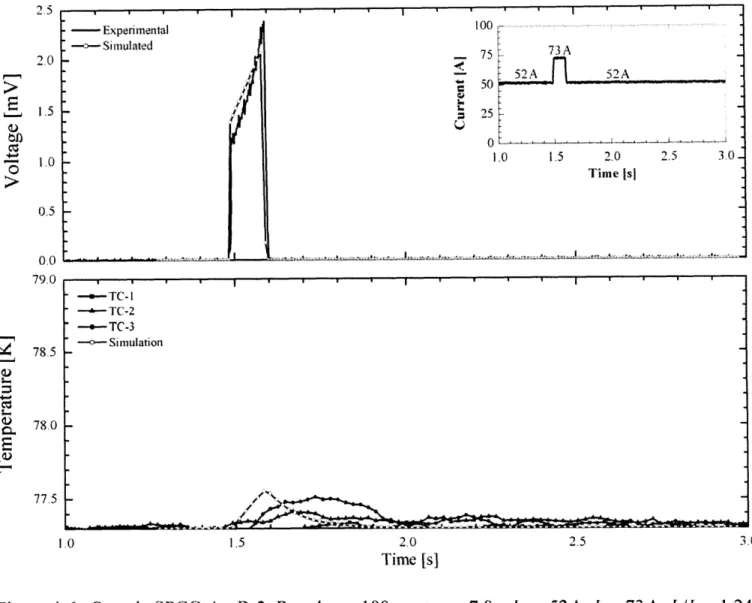
Virgin run for sample SPCC-Ag-B-2. Measured using both 5-cm and 10-cm voltage taps; Ic 5-cm = 58.5 A and Ic JOcm = 58.5 A

w ith a 1 pV/cm criterion...

Sample SPCC-Ag-B-2: Run 4, r = 100ms, thold = 7.0 s, Iop = 52A,

Ip = 73 A , I/Ic = 1.24... Critical current for sample SPCC-Ag-B-2 after 6th pulse.

Measured using both 5-cm and 10-cm voltage taps;

Ic 5-cm = 58.5 A and Ic ocm = 58.5A with a 1 pV/cm criterion...

Sample SPCC-Ag-B-2: Run 7, r = lOOms, thold = 7.0s,

Iop = 52A , Ip = 78A , Ip/Ic = 1.33... Layer arrangements in sample for AMSC Ag-Cu laminated

sup ercon ductor...

11 13 16 18 21 27 28 29 30 31 31 34 36 37 38 39 41 42 43 44 47

(8)

Figure 4-10. Figure 4-11. Figure 4-12. Figure 4-13. Figure 4-14. Figure 4-15. Figure 4-16. Figure 4-17. Figure 4-18. Figure 4-19. Figure 4-20. Figure 4-21. Figure 4-22. Figure 4-23. Figure 4-24. Figure 4-25. Figure 4-26. Figure 4-27.

Virgin run for sample CC52-335-LAM. Measured using 5-cm

voltage taps; Ic 5-c =129A with a 1 pV/cm criterion...

Sample CC52-335-LAM: Run 15, r = 150ms, thold =7.0s,

Iop = 117 A , I = 245 A , I /Ic = 1.90...

Sample CC52-335-LAM: Run 35, r= 150ms, thold =7.0s,

Io, = 117A , Ip = 552A , I/Ie = 4.30...

Critical current for sample CC52-335-LAM after 35th pulse. Measured using only 5-cm voltage taps; Ic Scm = 129 A with

a 1 tV/cm criterion...

Sample CC52-335-LAM: Predicted YBCO burnout, r= 150ms,

t_hold 7_{.0 S, Iop =}_117A,_{Ip = 80A, I/Ie = 6.27...} Virgin run for sample CC5 1 -R540-0- 10. Measured using only

5-cm voltage taps; Ic 5-cm = 11 OA with a 1 pV/cm criterion...

Sample CC51-R540-0-10: Run 21, r= 300ms, t

hold = 7.0s, Iop = 104A , Ip =500A , Ip/Ic = 4.55...

Critical current for sample CC5 1 -R540-0-10 after 21 t pulse. Measured using only 5-cm voltage taps; Ic 5-cm 110 A with

a 1 p V/cm criterion...

Sample CC51-R540-0-10: Predicted YBCO burnout, r= 300ms,

thold 7.0 s, Iop = 104A, Ip =665 A, Ip/Ic = 6.04...

Virgin run for sample CC84-755-8. Measured using both 5-cm and 10-cm voltage taps; Ic S-cm = 94A and Ic JOcm = 95A with

a 1 p V/cm criterion... Critical current for sample CC84-755-8 after 31St pulse.

Ic 5-cm= 91 A and Ic Jo-cm = 91 A with a 1 pV/cm criterion... Sample CC84-755-8: Run 32, r= lOOms, thold = 7.Os,

Iop = 80A, I = 360A, I/Ic = 3.96...

Critical current for sample CC84-755-8 after 3 7th pulse.

Ic 5-cm = 91 A and Ic Jo-cm= 91 A with a 1 pV/cm criterion...

Sample CC84-755-8: Run 38, r= 100ms, thold -7.0s, Iop = 80A,

Ip = 43 3 A, Ip/Ie = 4.76 ...

Layer arrangements in sample for SPI Ag-Cu laminated superconductor. Side copper layers electrically short upper and lower layers. The thickness of each side copper layer is not known exactly, though it is on the order of~10-pm... Virgin run for sample SPCC-Cu-A-1. Measured using both 5-cm

and 10-cm voltage taps; Ic Scm = 59.5A and Ic JOcm = 56.OA with

a 1 p V /cm criterion...

Sample SPCC-Cu-A-1: Run 2, r= 100ms, thold = 7.0 s,

Iop = 51 A , I> 100 A , I/Ic = 1.68... Sample SPCC-Cu-A-1: Run 12, T= 100ms, thold= 7.0 s,

Io = 51 A , Ip = l 355A , Ip/Ic = 5.92... 47 48 49 50 51 53 54 55 56 59 60 61 62 63 65 66 67 68

(9)

Figure 4-28. Critical current for sample SPCC-Cu-A-1 after 12th Pulse. Measured using both 5-cm and 10-cm voltage taps;

I, 5-m = 60.0 A and I, O-cm = 57.0 A with a 1 pV/cm criterion...

Figure 4-29. Sample SPCC-Cu-A-1: Run 13, r= 100 ms, th0ld = 7.0 s,

Io = 51 A , I = 404A , I,/Jc = 6.85...l

Figure 4-30. Critical current for sample SPCC-Cu-A- 1 after 13 t pulse.

Ic 5-cm = 58.5 A and Ic Jo-cm= 57.OA with a 1 tV/cm criterion...

Figure 4-31. Virgin run for sample SPCC-Cu-G. Measured using both 5-cm and 10-cm voltage taps; Ic 5-cm = 40.8 A and Ic Jo-cm = 40.5 A

w ith a I pV /cm criterion...

Figure 4-32. Sample SPCC-Cu-G: Run 4, r= 300ms, thold = 7.0s, op= 36A, Ip = 22 1 A , Ip/Ic = 6.13...

Figure 4-33. Sample SPCC-Cu-G: Run 11, z= 300ms, thold = 7.0s, Iop = 36A, Ip = 335A , Ip/Ic = 9.10...

Figure 4-34. Critical current for sample SPCC-Cu-G after 1 1 th pulse. Measured using both 5-cm and 10-cm voltage taps;

Ic S-cm = 39.3 A and Ic Jo-cm = 39.3 A with a 1 pV/cm criterion...

Figure 4-35. Sample SPCC-Cu-G: Run 12, r= 300ms, thold = 7.0s, Ip = 36A,

Ip = 370A , Ip/Ic = 9.4 8... . . . .. . . .. . . ....

Figure 4-36. Experimental and simulated II ratios for each sample... Figure 4-37. Simulated results for each sample using a 100-ms pulse and

400K burnout criterion...

Figure B- 1. Specific Heat of Copper 100 for 10K < T < 200K... Figure B-2. Specific Heat of Copper 100 for 200K < T< 1200 K... Figure B-3. Resistivity of Copper 100 for 20 K < T < 190 K... Figure B-4. Resistivity of Copper 100 for 190 K < T < 1300 K... Figure B-5. Specific Heat of Silver for 10K < T< 1200K... Figure B-6. Resistivity of Silver for OK < T< 293K... Figure B-7. Resistivity of Silver for 293 K < T < 1000K... Figure B-8. Specific Heat of YBCO for 77.3 K < T < 300K...

Figure C-1. LabVIEW code used to generate the pulse control for the power supplies. This was used with a voltage divider inline to the pow er supply signal... Figure C-2. LabVIEW code used to generate the pulse current signal. This

figure is the left portion, continued in Figure C-3... Figure C-3. LabVIEW code used to generate the pulse current signal. This

figure is the right portion, continued from Figure C-2... Figure D-1. Electrical Diagram for Sample to DAQ Connections...

69 70 71 72 73 74 75 76 77 78 94 94 95 95 96 96 97 97 98 99 100 101

(10)

List of Tables

Table 3.1 SCXI chassis configuration and filters settings... 33

Table 4-1. Specifications for 10-mm wide AMSC Ag stabilized samples... 36

Table 4-2. Specifications for 4-mm SPI Ag stabilized samples... 40

Table 4-3. Specifications for 1-cm wide Ag-Cu stabilized samples... 46

Table 4-4. Specifications for 4-mm wide Ag-Cu stabilized samples... 58

(11)

Chapter 1 Introduction

1.1 History of Superconductivity

1.1.1 Discovery

Kamerlingh Onnes first discovered superconductivity in 1911. After successfully liquefying helium in 1908, he was able to test the resistivity of several elements at 4.2 K

[1]. While conducting these experiments, he first noticed that the resistivity of pure

mercury was zero and went on to find the zero resistivity states for other elements, such as tin and lead, by 1914. Although this discovery was a major breakthrough, these early superconducting elements, designated Type I superconductors, exhibited several

disadvantages, the most significant ones being their low critical magnetic field and low critical current densities.

1.1.2 Definition of Superconductivity

Superconductivity is defined as the ability to conduct current without resistive losses [2]. Superconductors are governed by a critical surface relating the three properties

contributing to superconductivity: critical temperature (Tc), critical magnetic field (H), and critical current density (Jc). Although there are in-depth formulas governing their relations to each other, Figure 1-1 illustrates the general case.

J

f

2

(J,

T, Ho)

f3(J, H, To)

f

H

T

fi(HT,J = 0)

(12)

From Figure 1-1, it can be seen that as one property is increased, the other two must decrease for the superconductor to remain superconducting. Although most

superconductors have a critical temperature under 10K, modem research has developed the so-called "High Temperature Superconductors" (HTS), some of which have critical temperatures above 77K.

1.1.3 Type I Superconductors

Type I superconductors are often referred to as soft superconductors. A Type I

superconductor is the classification given to those first discovered by Kamerlingh Onnes, and are generally pure metals. These superconductors are unsuitable for magnet design because they have extremely low critical fields, generally less then 105 A/m, and the absence of a trapped magnetic field. Known as the Meissner effect, these

superconductors effectively shield out a magnetic field within the superconductor except over a thin layer at the surface [3].

1.1.4 Type II Superconductors

Often referred to as 'hard' superconductors, Type II superconductors were first

discovered in 1930 by Haas and Voogd when they combined an alloy of lead and bismuth [4]. Type II superconductors have normal islands in a sea of superconductivity known as the Abrikosov Vortex Lattice [5]. Compared to Type I superconductors, they have very high critical magnetic field and current densities due to this mixed magnetic state. Most Type II superconductors such as the intermetallic compounds of niobium tin and alloys of niobium titanium have critical temperatures below 20K. Modem superconducting

materials research continues to push the envelope higher, increasing the critical temperatures in HTS to as high as 140K.

1.2 High Temperature Superconductors

1.2.1 Types of High Temperature Superconductors

The advent of HTS came with the discovery of La-Ba-Cu-O in April of 1986 by Bednorz and Muller [5]. Their initial HTS had T, of 35K, and although the temperature was not as high as later copper oxide perovskites, it started a boom to discover better

superconductors with higher critical temperatures. Figure 1-2 shows the most common of the hundreds of HTS discovered since then.

(13)

- Space Temperatures

Liquid Nitrogen Temperature

P Hg-Ba-Ca-Cu-0

Q

TI-2223 OBi-2223 6 Bi-2212 Q YBa₂Cu₃07 50 -4 6 La-Ba-Cu-0 Nb₃Ge 0 BaKBiO3 NbN Nb3Sn g) Nb BaPbBiO3 Pb N. -Hg rrNWo Liquid He-0 1900 B I I 1950 2000 Year

Figure 1-2. Evolution of T, since the discovery of superconductivity [1 & 5].

1.2.2 Liquid Nitrogen Cooling

A significant advantage to HTS is that most can be used at a temperature as high as that

of boiling liquid nitrogen, while most low temperature superconductors (LTS) require operation at liquid helium temperatures, of which the major disadvantage is greater cryogenic costs compared with operation at liquid nitrogen temperatures.

1.3 Thermal Stability

The superconductor must remain under its critical surface to remain superconducting. Although keeping the superconductor under its critical temperature is ideal, in typical applications, there are times when the temperature of the superconductor momentarily will rise above the critical temperature of the superconductor. Known as being driven

150

--100 -f

U

(14)

"normal" or "quenching", the superconductor becomes resistive. In this case, there must be some type of stabilization to the superconductor. Stabilization, often in the form of embedding the superconductor in a highly-conductive normal metal matrix, such as silver or copper, provides a resistive current path. Without this stabilization, the superconductor would burn out and the device would fail.

When a current-carrying superconductor is driven normal, it has two possible responses: 1. It recovers, meaning the quench-induced heating is balanced by the external

cooling and the superconductor returns to the superconducting state. 2. It continues to generate heat, as heating exceeds cooling until the

superconductor and metal matrix eventually burn out.

In a stabilized superconductor, as the temperature of the superconductor increases, "current sharing" will occur between the superconductor and the matrix alloys until eventually the matrix carries the entire current. In this case, the stabilizing matrix must be able to carry the entire load current until the conductor can recover without being burnt out. A heating-and-cooling balance must be achieved to ensure that the

stabilization can carry the entire current of the sample if the superconductor is driven normal.

1.4 Overview

1.4.1 YBCO

This experiment will focus on coated YBCO, (yttrium barium copper oxide) with a critical temperature of 93K. YBCO is the first superconductor to remain

superconducting at liquid nitrogen temperatures. In the quest to develop better superconductors, this new ceramic has a higher critical current density then BSSCO superconductor.

The exponential slope of the V-I curve, referred to as the n-value of the superconductor, controls the rate at which the superconductor transitions to the resistive state. HTS, with lower n-values then LTS, are able to sustain current sharing over larger current ranges. The relations between current sharing, n-value, and temperature will be developed in Chapter 2.

1.4.2 Limits to Technology

Currently it is difficult to make coated YBCO conductors of length greater then 100m. Efforts are being made to develop tape on the order of 1 km. Manufacturing difficulties include aligning the YBCO biaxially and ensuring a uniform textured buffer layer. For alignment control, several processes have been developed including ion-beam assisted deposition (IBAD), inclined substrate deposition (ISD), and rolling-assisted biaxially textured substrate (RABiTS).

(15)

Although YBCO has high current density its quenching phenomenon must be understood before YBCO can be used in power applications [6]. With so many advantages over

BSSCO, companies are looking to use YBCO in magnets and other high current power

applications. However, before YBCO can be used effectively, the stability of the superconductor must be well understood when it is driven normal.

1.4.3 Experimental Focus

To ensure that the superconductor remains stable, a balance must be obtained between the heating and cooling governed by the power equation. The general form of which is given in Equation 1-1 for a conductor cooled by liquid nitrogen [7].

Vd Pd Cds

_at

=T-Vd -V{kdV T) + +Gj(T) - A, -qN, (T where,

Vd= Volume of the conductor [m3 ]

Pcd = Density of the conductor

Ce = Specific heat of the conductor [g K

T= Temperature [K]

t = Time _[s]

kcd = Thermal conductivity of the conductor m7K

Gj= Joule heating of the conductor _[W]

A,= _{Surface area of the conductor exposed to liquid nitrogen} _[m2

]

qN, = Liquid nitrogen cooling flux

[2W

Using this equation as a base, we will develop a model to predict the limit at which YBCO conductors laminated with copper remains stable after an over-current pulse condition. An experiment will then be performed to verify the results developed in the model. In addition, we will explore the stability requirements for copper laminated YBCO superconductor.

(16)

Chapter 2 Model for Liquid Nitrogen Cooling

2.1 Model for Quench and Recovery in YBCO Superconductor

In order to develop an analytical model to predict the quench and recovery of YBCO, a simulation was developed using MATLAB. In the following sections, the equations used to generate the model are derived and explained, beginning with the power equation, then developing the heat transfer, and concluding with material properties. The actual

program code for MATLAB is included in Appendix A.

2.1.1 Power Equation

The first place to begin with the development of a model for the thermodynamic behavior of a superconductor is through Equation 1-1. Expanding the conduction term for this equation in three dimensions yields Equation 2-1a:

aT

a

2

_T

_a

2

_T

_a

2

_T

PdCds -=Vk

+Vk

+VT kd kad2 2

+ Gj(T) - Aq (T)

(2-1a)

,at x ay Z

where,

kd = Thermal conductivity of the entire conductor in the ith direction, _mK

The orientation of the superconductor with current terminals and coordinate axis is shown in Figure 2-1.

z

Positive Current Terminal

Transport Current

Y

X

Negative Current Terminal

(17)

For copper and silver stabilized samples, the rate of conduction given by the characteristic time constant in Equation 2-2 is controlled largely by the thermal diffusivity [8].

te = (2-2)

a

where,

t, Characteristic time constant for conduction in the ith direction [s]

L Length of the sample in the i' direction [in]

a= Thermal diffusivity of conductor

[m2

Since silver and copper have extremely high thermal diffusivities, temperature changes in the entire conductor will propagate quickly. Consequently, the conductor is assumed to have uniform temperature in all three coordinate axes, and all the conduction terms cancel out of Equation 2-la to produce Equation 2-lb.

aT

Vc PCd Ccd = G(T) - AqN2-b)

at

With the simplified power equation, we can look specifically at the energy terms of the nitrogen cooling and joule heating. The cooling term given by qN, (T) is comprised of a conduction and convection term as shown in Equation 2-1c:

aT

- 2T

Vd Pcdcda

_at

= G(T)- A,h

AT-V

k

(2- c)

S 8lig

where,

hoV = Convective heat transfer coefficient [MWK]

VN= Volume of liquid nitrogen _[in3

kN2 = Thermal conductivity of liquid nitrogen in the ith (x, y, z) direction m-K

Since the liquid nitrogen is boiling as a saturated liquid, the temperature of the nitrogen in the x and y directions are uniform; therefore, these two conduction terms are neglected. Similarly, the conduction term in the z-direction is neglected due to the formation of the liquid-vapor boundary layer during natural convection and ultimately boiling as

conduction through this layer is very small. Eliminating these terms produces Equation 2-Id, leaving the dominating convective heat transfer term.

aT

Vcd Pd CC

a

= Gj(T)-

AshconN2

AT

(2-1d)

(18)

Standard published data for the convective heat flux of liquid nitrogen was used in the numerical analysis and will be discussed in Section 2.2.

The second to the last term in Equation 2-la is joule heating. This term comes from the dissipation of the current through the entire conductor matrix. If the current is less then the critical current of the superconductor, this term is zero. However, as the temperature of the conductor increases, current sharing with the resistive metal matrix produces Equation 2-le.

VpePCd

a

= R,,(T )- Ah, nv AT (2-1e)

at

where

I, =Total operating current in superconductor and metal matrix [A]

I, Current in the metal matrix [A]

Rm (T) = Resistance of the metal matrix

_[]

2.1.2 Parallel Resistance Model

A superconductor must be stabilized with a metal matrix in order to provide current a conductive path to flow when the superconductor is not superconducting. For this experiment, the size and composition of the silver and copper laminates can vary. To understand the behavior of a superconductor and its interaction with the metal matrix, a parallel resistor circuit model is used to describe the current sharing that occurs as the superconductor is energized. The circuit model for this is shown in Figure 2-2. It includes all three modes of current distribution as the temperature of the superconductor increases.

IOP

lim

Metal Matrix

O

Superconductor

Superconductor-Matrix Current Model for Iops:! IC

Im =

'op

-

Is

Matrix

Superconducting Region Current Sharing Region Pure Resistive Region

T_<_Tc _{TC : T : 93K} _{93K< T}

Figure 2-2. Circuit model for a composite superconductor. Above: Model for I, 5 I . Below: All three temperature ranges.

(19)

Below the critical temperature, the superconductor behaves like a short circuit as shown in the lower left most circuit model of Figure 2-2. As the current is increased above the superconductor's critical current, current sharing with the metal stabilizer occurs. As a result of the current sharing, there is resistive heating in the metal matrix, which, if not balanced by cooling causes the temperature of the conductor to rise. Due to increasing temperature, the voltage in the superconductor will rise with the onset resistivity. Since the superconductor is in parallel with the metal stabilizer, the voltage across the metal and superconductor must be the same, and is defined by Equation 2-3 [3].

V,(T)

=

L

I,

T)

(2-3)

where,

V, (T) Voltage in superconductor _[V]

V, = Critical voltage parameter described as 1p !V/cm [V]

I, = Current in the superconductor [A]

I, (T) = Critical current of the superconductor [A]

n = Index number for the superconductor

The critical current of the sample is measured experimentally in liquid nitrogen at 77.3 K, and for the simulation, is determined as a function of temperature using Equation 2-4 [9].

(

I

KT

I, (T) =-

)" xIn (T(2-4)

0.1848 77.3) where,

I'7 = Critical current measured in liquid nitrogen at 77.3 K [A]

Due to the effect of the superconductors index number, the actual current in the superconductor can be higher then the critical current at 77.3 K. The index number, defined by the experimentally measured values in Equation 2-5, control the

superconductor's voltage in the current sharing regime as the superconductor's current increases [3].

In (10)

n= -

5

(2-5)

In _._

where,

15. = Experimentally measured current when V, = 5.OpV [A]

10.5 = Experimentally measured current when V, = 0.5pV [A]

If the n-value is increased, the superconductor has a slower transition to the resistive state, and carries more current than a similar sample with a lower n-value at the same temperature. It is an important manufacturing goal to improve the n-value of HTS. Once the temperature of the YBCO rises above 93K, due to its high resistivity, the

(20)

superconductor is neglected form the model and the voltage characteristics are controlled exclusively by the electrical resistivity of the metal stabilizer.

2.1.3 Numerical Solution

A solution to the model is obtained by fixing the time interval, At = 0.001 s. At any (k)

time interval, the temperature of the conductor is determined by dividing the remaining heat not removed by the liquid nitrogen by the specific heat capacity of the conductor and adding this change in temperature to the previous interval's temperature. Due to the temperature dependence of the conductor's material properties, the resulting change in temperature produces a dynamic interaction that involves several iterations at each time interval to ensure the convergence of Equation 2-1 e.

2.2 Heat Transfer

2.2.1 Overview

In this experiment, the heat flux through the surface of the conductor is a function of the temperature of the surface. The heat transfer mechanisms for liquid nitrogen cooling are divided into two categories: natural convection and pool boiling. Natural convection occurs until the temperature of the tape forces the heat transfer into a pool boiling regime. Pool boiling is a complex heat transfer mechanism that can be divided into two regimes, nucleate and film boiling. Nucleate boiling starts when little droplets of vapor at the heater surface begin to nucleate on surface imperfections. As these vapor bubbles grow larger, they begin to depart from the surface of the heater when their buoyancy forces becomes significant.

As the heat flux from the heater is increased, the nucleate boiling will reach a maximum peak heat flux. This value occurs when the liquid down-flow to the surface cannot keep up with the rate at which the vapor bubbles leave the surface, resulting in the liquids inability to sustain a higher evaporation rate. Increasing the heat flux from the surface even slightly causes a dramatic jump in the surface temperature. Provided the input power remains constant, the maximum heat flux into the nitrogen will also remain constant. However, after a pulse, the power input decreases and as a result of this interruption in power flux, the nitrogen cooling can no longer sustain peak heat flux, and the cooling moves from the peak nucleate boiling regime into the film-boiling regime. From the maximum change in temperature where the peak nucleate boiling heat flux stops, the nitrogen cooling follows a gradual decrease through the film-boiling regime, which occurs when the nucleating bubbles begin to form a vapor layer satisfying Taylor wave criteria across the surface of the conductor. Although stable, the convective heat transfer from the film regime does not decrease all the way to zero. There is a minimum heat flux where the film regime will revert back to the nucleate boiling regime through a state of constant minimum heat flux. Figure 2-3 illustrates the typical published heat transfer data from liquid nitrogen as a function of the change in temperature of the heater surface.

(21)

2.2.2 Simulation Model for Liquid Nitrogen Heat Transfer

To model the heat transfer for a pulsed heat flux, an algorithm was developed using MATLAB. When the current is held constant before the pulse, the sample is cooled through natural convection. In order to simplify the calculations for the natural

convection heat transfer, the straight line shown in Equation 2-6a was adapted from the data of Merte and Clark to approximate the cooling through this regime [10].

qNC = 901.3115 x (AT x1.8) 77.3K T < 79.2K (2-6a)

where,

qNC = Natural convection heat transfer of liquid nitrogen, I W AT = Difference in temperature between sample and liquid nitrogen [K]

Typical heat flux used in simulation

-- Heat flux data adapted from Merte

Nucleate Bolling

4- Minin um

Natural C Onvetion~f

10

& Clark

1Peak I eat FluxI

Boiling 1000 100 10 - - - - Transition Boiline -H eat F lux ef - - -. .... -. ... .. .... ... ...

E

1 I 100

T -T , [K

_w _{sat, I}

Figure 2-3. Standard liquid nitrogen heat flux adapted from the data of Merte and Clark with a typical curve from the simulation superimposed [10].

When the pulse is large, the natural convection regime transitions to the nucleate boiling regime. Since the maximum heat flux changes with pulse amplitude, it was determined that the temperature where the transition from nucleate boiling to the peak heat flux could range between 85-90 K. Using 88 K as a reference transition temperature to the maximum

(22)

heat flux - 3 was added to this temperature. Adapted from the data of Merte and

Clark, Equation 2-6b was used to define the nucleate boiling regime of the heat transfer [10].

qNB=

207.8875

x (AT*1 .8)2.1709 79.2K T < 88 +

(I,/I

-

3)]

K (2-6b)

where,

qNB=

Nucleate boiling heat transfer of liquid nitrogen

[

Once the temperature of the sample exceeds the transition temperature for the peak heat flux, the temperature will continue to rise, but cooling will remain constant until there is an interruption in power or the sample bums out. The peak nucleate boiling heat flux, shown in Equation 2-6c, was adapted from the data presented by Merte and Clark [10].

qNBea. = 207.8875 x

{1

.8x

[10.7+(II,

-3 2.1709 88 +

(I

c

-3 ! T < TP, (2-6c)

where,

qNBak= Peak nucleate boiling heat transfer of liquid nitrogen,

W

T

Peak = Peak Temperature after pulse ends [K]

After the pulse, the power is interrupted and a maximum temperature is reached. At this point, the liquid nitrogen is unable to sustain peak heat flux and transitions to the film-boiling regime. Based on the material presented by Titus, I have chosen a film-film-boiling curve that follows a line parallel to the data presented by Bromely et al., but starts at the peak heat flux and maximum temperature immediately after the pulse [11]. The heat transfer to the liquid nitrogen for the film-boiling regime, described by Equation 2-6d, was adapted from the data presented by Merte and Clark [10].

qFilm = 3.15459 x qNB. X (AT x 1.8)0.7686 Peak - Trans, (2-6d) Peak0.7686

where,

qFilm = Film boiling heat transfer for liquid nitrogen

]

(23)

As the sample cools the heat transfer will remain in the film-boiling regime until it intersects the transition heat flux line defined by Equation 2-7, adapted from the standard boiling data of Merte and Clark [10]:

qrans = 2.52367 x 1024

(AT x

1.8)11958 99K T >108K (2-7)

where,

qmrans = Transition boiling heat transfer

[

When Equation 2-6d intersects Equation 2-7, the heat flux will remain constant at the minimum film boiling heat flux for the temperature range shown in Equation 2-6e, which was adapted from the data presented by Merte and Clark [10].

q N P<. 1 .8] 0 .7686 T

-6 e )

qFilm,, =

3.15459 x

TNB0.7686 X Trans, .X

T

>

Tran Peak

where,

qFilm . = Minimum film boiling heat transfer for liquid nitrogen

2

TTrans = Transition temperature where Equation 2-6e and 2-6b intersect [K]

Minimum film boiling heat flux will continue until Equation 2-6e intersects Equation 2-6b. From that intersection, the sample will continue to cool and the heat flux to the liquid nitrogen will pass back through the nucleate boiling and natural convection regimes, eventually reaching zero.

Equation 2-6 was incorporated into the MATLAB code. However, the equations for the material properties as functions of temperature were designed to run as stand-alone scripts that could be called in the main MATLAB program. Isolating these components streamlined the code to run efficiently, and they were easily modified as more accurate material data became available.

2.3 Copper Properties

This section presents piecewise equations for copper properties created from published data.

2.3.1 Specific Heat of Copper

The following equations, based on published data [8, 12] are used for specific heat of copper, CuCp [J/kg -K].

(24)

CuCp

=368.53324 (1

-

e-.0

23 22T)3.65205 10K T < 200K CuCp = 2.3181 x 10-7T3 _- _0.00052T2 + 0.44648T + 287.47602 200K ! T <1200K (2-8a) (2-8b)

Reference data and the supporting curve fit from OriginPro are provided as a supplement

in Appendix B.

2.3.2 Resistivity of Copper

The resistivity of copper, CuRes [nQ -m] was also tabulated from cryogenic and room temperature sources [3, 13]. CuRes = -1.1787 x10-6 T3 _+0.00067T 2 _{-0.02399T +0.3855} (T+2715.04572 CuRes = 34.4038e( 2191.4633 )-118.11359 20K: T <190K (2-9a) 190K T <1300K (2-9b) Reference data and the supporting curve-fit from OriginPro are provided as a supplement

in Appendix B.

2.4 Silver Properties

2.4.1 Specific Heat of Silver

Tabulated data for the specific heat of silver, AgCp [J/kg -K] were curve-fit from cryogenic and room temperature sources to produce Equation 2-10 [8, 14].

AgCp = 571302.22046T000 " -571442.51725 1OK < T <1200K (2-10)

Reference data and the supporting curve-fit from OriginPro are provided as a supplement in Appendix B.

2.4.2 Resistivity of Silver

Similarly, Equation 2-11, a piecewise function for the resistivity of silver, AgRes [nQ -m] was determined from a curve-fit of cryogenic and room temperature data [3, 13].

AgRes = -1.0796 x10- T3 _+0.00046T2 _{+0.01555T -0.38874}

AgRes = 00685T -3.77476

OK ! T < 293K (2-1 la)

293K ! T <1000K (2-1lb)

Reference data and the supporting curve-fit from OriginPro are provided as a supplement

(25)

2.5 Material Properties of Substrate

The substrate used in both the American Superconductor Inc. (AMSC) and SuperPower Inc. (SPI) tapes were derived from nickel alloys. The AMSC substrate was composed of nickel with 5%W RABiTS, while the SPI substrate was composed of Hastaloy C. The specific heat of nickel, CpN [J/kg K] is used for both substrates because of their high nickel content. Equation 2-12 is a piecewise construction of the specific heat of nickel, comprised from cryogenic and room temperature data [8, 15].

CpNi = 8890 X 1 015,503.108-37,280.377 Log(T)+26,788.417 Log(T)2 +7,010.0877Log(T)

3 ...

-22, 731.65lLog(T)4 + 15, 386.526Log(T) - 5, 175.7968Log(T)

+896.97274Log(T) -64.055866Log(T) 55K T 300K (2-12a)

CpNi =8,890

x(0.1581T +410.24)

300K<T (2-12b)

Since Equation 2-12a was provided by NIST, the curve-fit data associated with the material properties is not required whereas Equation 2-12b was derived from the linear interpolation of the tabulated data from Mills [8, 15].

2.5.1 AMSC Substrate Resistivity

The resistivity, SubResMsc [nK -m] shown in Equation 2-13 for nickel with 5%W

RABiTS substrate, was provided by AMSC [9].

SubResAMSC = 4.717 xI0

'T+2.28491x10-7

77K s

T <1000K

(2-13)

2.5.2 SPI Substrate Resistivity

In contrast, for the SPI samples, the resistivity was measured in the lab at both liquid nitrogen and room temperatures. However, since there was very little variation between the cryogenic and room temperature resistivity, a constant value of SubResspj

1.30 x 10-6[nK2 -m] was used for all temperature ranges.

2.6 Material Properties of YBCO

2.6.1 Specific Heat of YBCO

Due to the effect of the short coherence lengths YBCO superconductor can have local fluctuations in and out of the superconducting state without affecting the entire tape. The effects of the local fluctuations in and out of the superconducting state can be seen in the specific heat, thermal conductivity, and magnetic susceptibility of the sample. Each of these properties change anomalously around the superconducting transition temperature

of the sample [16]. In particular, the specific heat of YBCO has two distinct jumps near its superconducting transition temperature.

(26)

Aravind and Fung attribute the dip in the thermal diffusivity at the onset of resistivity to an abrupt increase in the electron specific heat as the sample moves from the resistive to superconducting states within the individual grains. They further speculate that the increase in the thermal diffusivity below the critical temperature is due to the increase in the mean free path of photons, which occurs as the charge carriers condense to form Cooper pairs [16].

Aravind and Fung have developed the most thorough results for the cryogenic specific heat of YBCO, CpYBCO [J/kg -K]. Equation 2-14a-f is a piecewise curve-fit combining their data with the data of Roulin et al. [16, 17].

CPYBCO =1.2173T +91.659 77.4K < T ! 80.5K (2-14a) CPYBCO

= -19.423T +1752.4

80.5K

< T !

84K (2-14b) CpYBCO = 5.066 1T -304.24 84K < T ! 90K (2-14c) CPYBCO = -3.9285T

+504.7

90K

< T !

92K (2-14d) -T CPYBCO = -456.60151x

e

65.99887 _+260.40759 _{92K < T 200K} (2-14e) CPYBCO

=-0.0183T2

+1.254T

-1281.1

200K

< T !

300K (2-14f)

Equally important to the specific heat data at cryogenic properties are those between 300-1000K. Most studies into YBCO stability neglect these room temperature

properties, but the present study shows that these are in fact the most relevant values for the heat transfer from a pulsed conductor. Through the pulse induced quench process, the sample exceeds the cryogenic temperature range within a few milliseconds. After

reaching room temperatures, the sample then remains well above cryogenic temperatures for more then a few seconds. Consequently, these room temperature material property values dramatically influence the quench recovery criteria.

Matskevich and Stenin show an additional anomaly in the specific heat near 500 K [18]. The behavior of the specific heat in this region may explain why the superconductor appears to degrade around this temperature range. The anomalies in these measurements coincide with previous data taken for the linier-expansion coefficient by White et al. [19]. Matskevich and Stenin propose that the additional phase transition at 500K is due to the elongation of the bonds in the Cu2-04 layers. They also concluded that the temperature

for these anomalies change depending on the amount of apical oxygen doping in the CuO2 plane.

On the range of 300-900K, Matskevich and Stenin define the specific heat by Equation 2-14g-h [18]:

CPYBCO = 334.68 -0.28854T +5.7220 x10-4T2 _{300K < T 5 500K} _(2-14g)

CPYBCO = 316.92 -0.10258T +1.9478 x10-4T 2 _{500K <}_{T 5}_900K _(2-14h)

For the specific heat of YBCO, the supporting curve-fit for the cryogenic values from OriginPro are provided as a supplement in Appendix B.

(27)

Chapter 3 Experimental Verification of Model

3.1 Experimental Setup

3.1.1 Sample and Fixture

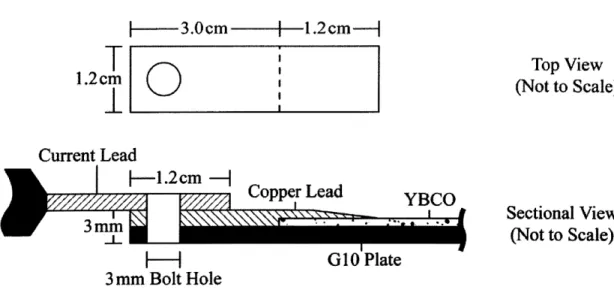
To ensure that each sample had the same orientation during each experiment, a fixture was fabricated to hold the samples in a liquid nitrogen bath. Copper current leads were connected to the sample. These leads, shown in Figure 3-1, allow the power supply cables to be bolted to the sample. The copper current leads provide a 1.5-cm overlap for the power supply cable lugs and a 1.2-cm overlap on the YBCO tape.

3.cm

-.

2cm-T

Top View

1.2cm

0 _{(Not to Scale)}

Current Lead

11.2cm

-Copper Lead

_YBCO

Sectional View

(Not to Scale)

-|G G10 Plate

3mm Bolt Hole

Figure 3-1. Copper leads to connect power supply lugs to YBCO sample. In order to mount the sample to the copper current leads and minimize the contact resistance, the following procedure was used, as adapted from AMSC [20]:

1. Set soldering iron to 200 C to prevent overheating and damage to sample 2. Using Tix flux, tin the copper leads and the top of YBCO sample with Indium

(66%) and Bismuth (33%) solder

3. Wipe leads and sample to remove excess flux with alcohol

4. Applying heat to the back of the sample, press it into the solder on the copper leads

5. Re-swab sample and current leads with alcohol to remove excess flux

After the sample was mounted onto the current leads, it was reinforced with a G- 10 plate. The G- 10 plate provided a stable base for the sample and allowed additional space for other components including the thermocouples and voltage tabs. The complete assembly,

(28)

shown in Figure 3-2, illustrates the three large clamps for the thermocouples, a thermocouple reference node, and the power supply's copper current leads. It is also important to note that the G- 10 plate acts as a thermal insulator to the backside sample, which is treated as adiabatic.

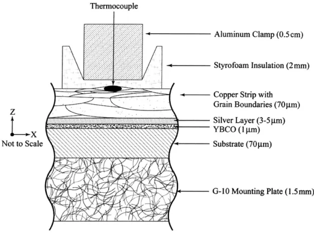
Gold-Chromel thermocouples were used for the temperature measurements of the sample. Each thermocouple was clamped on the sample's surface and electrically insulated with a 25-tm layer of Kapton tape. To insulate the thermocouple from the liquid nitrogen, it was covered with a 2-mm thick Styrofoam sheet.

Thermocouple Clamps

+ Current Lead G-10 Sample - Current Lead

A,'' T' T IA,

Section View from Side

Thermocouple Clamps

G-10 YBC0 Sample Tape

Current Lead Current Lead

I Ocm V+ 5cm V+ 5cm I Ocm

V--Thermocouple Reference

Top View

Figure 3-2. Complete sample holder and test assembly for liquid nitrogen cooling, shown in approximate scale except sample thickness, which has been exaggerated to show detail.

(29)

Trillaud et al. note that clamping the thermocouples would cause tiny imperfections in the

surface of the YBCO that reduce the current capacity of the tape [21]. However, our test

samples have shown there is no degradation in the current capacity. The absence of

current degradation may be attributable to the presence of the copper lamination. The

clamp assembly is shown in Figure 3-3 with enlarged details of the individual

components. To achieve uniform clamping pressure between experiments, screws

holding the thermocouple clamps were hand tightened to approximately the same torque.

Thermocouple

Aluminum Clamp (0.5cm)

Styrofoam

Insulation

(2mm)

Copper Strip with

Grain Boundaries (70pm)

Z

Silver Layer (3-Sm)

YBCO(I gm)

Not to Scale \ Substrate (70 m)

G-10 Mounting Plate (1.5mm)

Figure 3-3. Detailed sectional side view of thermocouple clamp system and the

absorption of the pressure from the thermocouple into copper stabilizer and

Styrofoam.

A reference temperature node for each thermocouple, at boiling liquid nitrogen (77.3 K),

was attached to the side of the G- 10 sample holder. At these reference nodes, the

thermocouples were attached to the copper signal wires that are connected to the data

acquisition (DAQ) system.

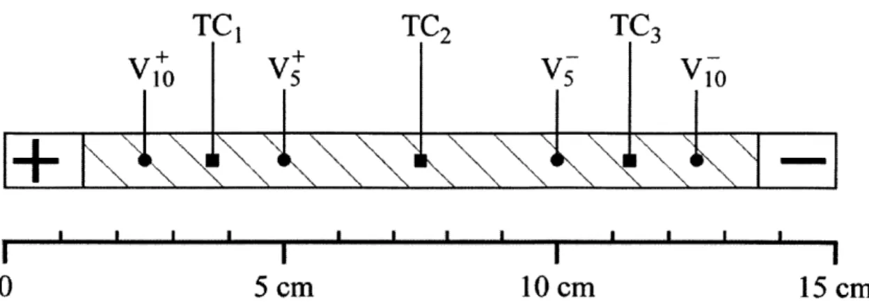
Two sets of voltage taps were soldered to the samples, one set 5-cm apart and the other

10-cm apart. The location of the voltage taps and thermocouples mounted on the YBCO

sample are schematically shown in Figure 3-4.

(30)

TC

1

TC

2

TC

3

I

0 5 cm

10 cm

15 cm

Hatched surface exposed to liquid nitrogen cooling

Figure 3-4. Location of voltage taps and thermocouples on 15-cm long YBCO sample.

3.1.2 Experimental Procedure

In order to quench the YBCO sample it was subjected to an over-current pulse. First, the sample remains superconducting at an operating current, set at 90% of the critical

current. This represents a typical operating condition. The sample is then subjected to an over-current pulse that drives the entire length of the sample to a normal resistive state. After the pulse, the current is reduced to the initial operating current. The pulse

amplitude ranged 2-12 times the critical current.

Before each pulse run, the sample's critical current, an electric field criterion of 1 piV/cm, was measured. From this, we determined the n-value of the superconductor [3]. The critical current was measured before each pulse run to determine if the sample experienced degradation during the previous run.

Figure 3-5, shows a typical current vs. time function used in the measurement. In this experiment, a square pulse of duration (ruse) in the range 100-10OOms was used. The quench behavior during and after the current pulse was recorded. In order to generate an over-current pulse of up to 600 A, six 100-A power supplies (HP6260B) were connected in parallel.

(31)

400

4)

U

200

0

0.5

1.0

1.5 Time [s]

Figure

3-5.

Typical current pulse generated by HP6260B power supplies for experiment.

HP Power Supplies (Lower Six Supplies

DAQ & Computei

r System

77.3K T

Figure 3-6. Experimental setup with power supplies, DAQ, and test setup.

'Pulse

'hold =0-901,

(32)

The power supplies were controlled with a voltage-programming signal generated in LabVIEW. LabVIEW was set up to allow synchronous power supply programming with data acquisition. The LabVIEW system is detailed in the following sections and an overview of the experimental setup is shown in Figure 3-6.

3.2 Data Acquisition System

3.2.1 Equipment and Setup

A National Instruments 12-bit PCI-AT-MIO- 1 6E data acquisition (DAQ) card was used

to synchronize and control the analog input and output for the experiment. With this

DAQ card, two separate control systems were created for the analog output. The first

provided a slow current ramp signal to the power supplies, while the second provided the programmable holding current and pulse.

For the current ramp program, a signal wire with a voltage divider was used to connect the DAQ output to the power supply's programming signal. By using the full DAQ output scale and a voltage divider, we were able to ramp the current as slow as 0.5 A per

second. The voltage divider introduced an RC interaction within the programming circuit that caused the power supplies to compensate and ramp according to the program

requirements [22]. To control the pulse current, a regular signal wire without a voltage divider was used, and this had to be switched with the other signal wire depending on the desired test mode. A separate LabVIEW code was also generated to ensure the proper output voltage signal.

Together with an SCXI-1000 chassis, LabVIEW 7.1 software was used to collect and interpret the experimental data. The SCXI chassis was configured with one SCXI-1 120D and two SCXI-1 120 modules, which allowed the user to configure individual gain and filter settings for each channel. Connected to these modules, SCXI-1320 terminal blocks were used for input connections. Table 3.1 lists the configurations used for this

experiment and their corresponding signal sources.

Although there were only two input voltage signals from the voltage taps, one 5-cm taps and the other 10-cm taps, eight channels were used to record a set of data. The signal from each channel was recorded at four amplification settings to avoid saturation of the

DAQ channels. For the over-current pulse experiments, it was determined that the best

filtering was a 1 0-kHz low-pass filter on each voltage signal. In contrast, a 4-Hz filter with a gain of 1000 was used for the voltage measurements in determining the critical current, however, the rest of the signals were measured with a 10- kHz low-pass filter. To verify the signal range and acquired values, Keithley 155 multimeters were used to monitor the signals in addition to the LabVIEW system.

(33)

Table 3.1 SCXI chassis configuration and filters settings.

I

Channel

I

Gain

I

Low-Pass Filter Frequency

I

Signal

1-1 100 4.5kHz Shunt resistor across power supplies

Module 2 SCXI- 1120

Channel Gain Low-Pass Filter Frequency Signal

2-0 1 10kHz 5-cm Voltage tap -Pulse experiment

2-1 10 10kHz 5-cm Voltage tap -Pulse experiment

2-2 100 10kHz 5-cm Voltage tap -Pulse experiment

2-3 1000 10kHz 5-cm Voltage tap -Pulse experiment

2-4 1 10kHz 10-cm Voltage tap -Pulse experiment

2-5 10 10kHz 10-cm Voltage tap -Pulse experiment 2-6 100 10kHz 10-cm Voltage tap -Pulse experiment

2-7 1000 10kHz 10-cm Voltage tap -Pulse experiment

Module3 SCXI-1120

Channel Gain Low-Pass Filter Frequency Signal

3-0 1000 4Hz 5-cm Voltage tap -Ramp experiment

3-1 1000 4Hz 10-cm Voltage tap -Ramp experiment

3-2 100 10kHz Thermocouple one 3-3 1000 10kHz Thermocouple one 3-4 100 10kHz Thermocouple two 3-5 1000 10kHz Thermocouple two 3-6 100 10kHz Thermocouple three 3-7 1000 10kHz Thennocouple three

Module 4

Analog

Out ut Hardwired from DAQ Card

Channel Gain Filter Frequency Signal

AO-0 - - Analog output voltage for pulse control

AO-1 - - Analog output voltage for ramp control

3.2.2 Software Analysis

Both the LabVIEW control programs for the ramp and over-current pulse were designed

to write an analog output for each point the DAQ acquired. The scan and output rate was

set to 1.0-kHz, which allowed the use of 0.001 s discretizations in the simulation. The

code used for each of these LabVIEW applications are provided in Appendix C. Once

the data were written to a text file, OriginPro was used to plot the data. To enhance the

clarity the thermocouple data were smoothed with a 100-point adjacent averaging

technique.

(34)

3.3 Block Diagram

The block diagram for the experiment is shown in Figure 3-7. The components and their connections to each other are illustrated, but the specific wiring diagram between the sample and the DAQ system are shown in Appendix D.

Convective heat transfer model for determining quench recovery of high temperature superconducting YBCO in liquid nitrogen

Convective Heat Transfer Model for Determining Quench

Recovery of High Temperature Superconducting YBCO in

Liquid Nitrogen

by

Joseph Edward Jankowski

B.S. in Mechanical Engineering

Loyola Marymount University, 2002

Submitted to the Department of Mechanical Engineering in partial

fulfillment of the requirements for the degree of

Master of Science in Mechanical Engineering

at the

MASSACHUSETTS INSTITUTE OF TECHNOLOGY

September 2004

© Massachusetts Institute of Technology 2004.

Author

All Rights Reserved.

/

'~i

/6~//

Department of Mechanical Engineering

August

23, 2004

Certified by

Dr. Yukikazu Iwasa

Thesis Supervisor

Accepted by

Ain A. Sonin

Chairman, Departmental Graduate Committee

Convective Heat Transfer Model for Determining Quench

Recovery of High Temperature Superconducting YBCO in

Liquid Nitrogen

By Joseph Edward Jankowski

Abstract

Acknowledgements

Table of Contents

List of Figures

List of Tables

Chapter 1

Introduction

1.1 History of Superconductivity

1.1.1 Discovery

1.1.2 Definition of Superconductivity

J

f

(J,

T, Ho)

f3(J, H, To)

f

H

T

fi(HT,J = 0)

1.1.3 Type I Superconductors

1.1.4 Type II Superconductors

1.2 High Temperature Superconductors

1.2.1 Types of High Temperature Superconductors

Q

1.2.2 Liquid Nitrogen Cooling

1.3 Thermal Stability

1.4 Overview

1.4.1 YBCO

1.4.2 Limits to Technology

1.4.3 Experimental Focus

at

[2W

Chapter 2

Model for Liquid Nitrogen Cooling

2.1 Model for Quench and Recovery in YBCO Superconductor

2.1.1 Power Equation

aT

a

T

a

T

a

T

+Vk

+ Gj(T) - Aq (T)

(2-1a)

z

_at

_T

_a

_T

_a

_T

_at

_[]