HAL Id: hal-01379733
https://hal.inria.fr/hal-01379733
Submitted on 17 Oct 2016
HAL is a multi-disciplinary open access
archive for the deposit and dissemination of
sci-entific research documents, whether they are
pub-lished or not. The documents may come from
teaching and research institutions in France or
L’archive ouverte pluridisciplinaire HAL, est
destinée au dépôt et à la diffusion de documents
scientifiques de niveau recherche, publiés ou non,
émanant des établissements d’enseignement et de
recherche français ou étrangers, des laboratoires
Formal Derivation of Qualitative Dynamical Models
from Biochemical Networks
Wassim Abou-Jaoudé, Denis Thieffry, Jérôme Feret
To cite this version:
Wassim
Abou-Jaoudé,
Denis
Thieffry,
Jérôme
Feret.
Formal
Derivation
of
Qualita-tive Dynamical Models from Biochemical Networks.
BioSystems, Elsevier, 2016, pp.100.
�10.1016/j.biosystems.2016.09.001�. �hal-01379733�
Formal Derivation of Qualitative Dynamical Models
from Biochemical Networks
IWassim Abou-Jaoud´ea,b,⇤, Denis Thie↵rya, J´erˆome Feretb,⇤
aComputational Systems Biology team, Institut de Biologie de l'Ecole Normale Sup´erieure
(IBENS), CNRS, Inserm, Ecole Normale Sup´erieure, PSL Research University, F-75005
Paris, France
bDI-ENS (INRIA/ ´ENS/CNRS/PSL?), Paris, France
Abstract
As technological advances allow a better identification of cellular networks, large-scale molecular data are swiftly produced, allowing the construction of large and detailed molecular interaction maps. One approach to unravel the dy-namical properties of such complex systems consists in deriving coarse-grained dynamical models from these maps, which would make the salient properties emerge. We present here a method to automatically derive such models, relying on the abstract interpretation framework to formally relate model behaviour at di↵erent levels of description. We illustrate our approach on two relevant case studies: the formation of a complex involving a protein adaptor, and a race between two competing biochemical reactions. States and traces of reaction networks are first abstracted by sampling the number of instances of chemical species within a finite set of intervals. We show that the qualitative models induced by this abstraction are too coarse to reproduce properties of interest. We then refine our approach by taking into account additional constraints, the mass invariants and the limiting resources for interval crossing, and by intro-ducing information on the reaction kinetics. The resulting qualitative models are able to capture sophisticated properties of interest, such as a sequestration e↵ect, which arise in the case studies and, more generally, participate in shap-ing the dynamics of cell signalshap-ing and regulatory networks. Our methodology o↵ers new trade-o↵s between complexity and accuracy, and clarifies the implicit assumptions made in the process of qualitative modelling of biological networks.
1. Introduction
As technological advances allow a better identification of cellular networks, more and more molecular data are produced enabling the construction of
de-IThis material is based upon works sponsored by the “´Ecole normale sup´erieure” (´ENS)
under an incitative action and by the Defense Advanced Research Projects Agency (DARPA) and the U. S. Army Research Office under grant number W911NF-14-1-0367. The views, opinions, and/or findings contained in this article are those of the authors and should not be interpreted as representing the official views or policies, either expressed or implied, of the
“´Ecole normale sup´erieure”, the Defense Advanced Research Projects Agency, or the U. S.
Department of Defense.
tailed molecular interaction maps. These maps form large and complex in-tertwined biochemical networks, which dynamical functioning is very hard to decipher. One approach to unravel the dynamical properties of such systems relies on the derivation of qualitative dynamical models from these maps, in order to ease the analysis of their dynamics [1, 2].
In qualitative modelling, the quantity of a biochemical species is usually modeled by a qualitative discrete level representing a range of concentration (or activity) of the component (rather than the exact number or concentration). Logical rules then specify the evolution of each component level depending on the other ones. Such rules can be defined as logical functions (as it is done in logical modelling [3]), or they can directly encode sets of reactions denoting molecular consumption and production processes (as it is the case in the Boolean semantics of BIOCHAM [4]).
Automatic methods for model derivations still lack of convenient trade-o↵ between efficiency and accuracy. Some abstractions consist only in partitioning the state space (as in the Boolean semantics of BIOCHAM [4]). These abstrac-tions are usually too conservative and fail in detecting properties of interest. They have to be refined by integrating an approximated quantitative descrip-tion of the dynamics of the model in each partidescrip-tion class, as done in tropical approximations [5] and piecewise affine systems [6]. Yet, the latter methods pro-vide no explicit bounds for numerical errors (at best an asymptotic estimation of them).
Our motivation is twofold: not only we want to design an automatic tool to derive accurate coarse-grained discrete models from reaction networks, but also we want to better understand the process of qualitative modelling and its underlying implicit assumptions. To achieve these goals, we use abstract in-terpretation. Abstract interpretation has been introduced forty years ago as a mathematical framework to formally relate the behaviour of programs or mod-els, seen at di↵erent levels of abstraction. Since then, abstract interpretation has been used not only to establish formal comparisons between abstraction tech-niques [7], but also to develop static analyzers that abstract automatically the behaviour of programs or models [8, 9]. Abstract interpretors are now spreading across the industrial community (for instance, companies as MicroSoft, Google, Facebook, and The Mathworks have been developing their own abstract inter-pretors).
The abstract interpretation framework is based on the idea that the be-haviour of a program or a model can be described formally as the least fixpoint lfpF of a monotonic operator F over the elements of a so-called concrete domain D, which is usually the set }(S) of the subsets of a given set S of elements. Then, an abstraction is a change of granularity in the description of the behaviour of the programs and the models, that can be mathematically formalized by vari-ous means, such as upper closure operators, ideals, Moore families, and Galois connections. In this paper, we use Galois connections, because it is the most popular means to describe an abstract interpretation. A change of observation level can be described by introducing a domain D] of properties of interest,
that is ordered by a partial order v. Each element a] of the abstract domain
D] is then related to the set of the concrete elements (a])
2 S that satisfy this abstract property, the so-defined function being monotonic. An abstract element a] is called an abstraction of a given set a of concrete elements, if and
only if, a ✓ (a]). A Galois connection is obtained when each subset a
has a most precise abstraction, that is to say that for any subset a✓ S, there exists an abstract element ↵(a) such that, for any other abstraction a] of the
element a, we have ↵(a) v a]. In this case, the function ↵ F is the best
abstract counterpart to the function F. Moreover, any monotonic function F]
over the abstract domain D] such that [↵ F ](a])
v F](a]), for each
ele-ment a]
2 D], satisfies lfp F ✓ (lfp F]), that is to say that the behaviour of
the program or the model can be carried out in the abstract domain, and the result is a sound over-approximation. By soundness, we mean that we miss no concrete behaviour. Yet our result may be approximate when the inclusion is strict, meaning that, because of the over-approximation, our abstraction has introduced spurious behaviours.
Sound over-approximations should not be confused with numerical approx-imations. A numerically approximated computation provides a behaviour that is close (hopefully) to the behaviour of the concrete program or model. However even with asymptotic guarantees, without an explicit bound of the numerical error, it is not possible to bound the e↵ective values of the variables in the ini-tial exact model. In contrast, the abstract interpretation framework has been used to develop certified numerical integration engines, in order to provide a sound over-approximation of the values of the variables in hybrid systems, by the means of couples of functions respectively for the lower and upper bound of the e↵ective value of the variables [10].
It is important to make the distinction between the properties that can be derived by the abstraction, and the underlying assumptions coming from the modelling paradigm. Indeed, the choice of the initial semantics is crucial, and it usually depends on the kind of modelling framework we are using. There is no ideal semantics. Even the concrete semantics is a trade-o↵ between what we can or want to observe about the execution of programs or models. Especially, it is important to fix the assumptions that explain how to solve competitions between potential reactions at di↵erent rates. There are di↵erent propositions in the literature according to the community. In this paper, we focus on the underlying assumptions that have been used in logical modelling [13].
Our approach is the following. In Section 3, we formalise the behaviour of reaction networks by keeping the exact number of instances of chemical species. In Section 4, we propose an abstraction in which the number of instances is sampled within a finite set of intervals. In Section 5, we refine this abstraction by taking into account three kinds of properties: we deal with mass preservation invariants in Section 5.1; we detect when the number of instances of a given chemical species cannot cross its sampling intervals in Section 5.2; we enrich the description of the behaviour of the models with information about the reaction rates and take into account the separation between time-scales in Section 5.3. Finally we show the applications of our refined abstraction on our case studies in Section 6.
2. Case studies
Firstly, we consider a model with three kinds of proteins A, B and C. We assume that the protein B is an adaptor between the proteins A and C, that is to say that each instance of B can bind to an instance of A and/or to an instance of C. We wonder what is the influence of the initial concentration of the protein B on the concentration of the trimer ABC. Intuitively, the more Bs we put
in the model, the more ABCs will be formed. Yet this is not the case, since at high concentration, the protein B prevents the proteins A and C to meet since almost each instance of A (resp. C) belongs to a dimer AB (resp. BC), and thus there is no available As (resp. Cs) to form the trimers ABC. Thus, at high concentration, by sequestration e↵ect, the adaptor prevents the formation of trimers ABC.
Figure 1 lists the reactions of the model (Fig. 1(a)), the system of equations (under the assumptions of the law of mass action) (Fig. 1(b)), and the concen-tration of the trimer ABC when the reactions have run to completion with respect to the initial concentration of the protein B (Fig. 1(c)). We notice that at low concentration of the protein B, the concentration of the trimer ABC grows linearly, whereas it drops following an homographic function at high con-centration of the protein B. Interestingly, this sequestration e↵ect has also been observed in vivo [11].
Secondly, we consider a model also involving three kinds of proteins A, B, and C. We assume that the protein A can be turned into protein B or C. More precisely, we assume that the production of an instance of B requires only one instance of the protein A, whereas the production of an instance of C requires two instances of the protein A. Here we wonder what is the influence of the initial concentration of the protein A on the concentration of the proteins B and C. Intuitively, the more A we put in the model the more C will be produced from the binary reaction compared to the production of B from the unary reaction. Therefore, at high (resp. low) concentration of A, the binary (resp. unary) reaction preempts the unary (resp. binary) one.
Figure 2 lists the reactions of the model (Fig. 2(a)), the system of equations (under the assumptions of the law of mass action) (Fig. 2(b)), and the concen-tration of the ratio between the concenconcen-tration of the proteins C and B when the reactions have run to completion with respect to the initial concentration of the protein A (Fig. 2(c)).
These examples are well suited for testing the accuracy of our approach, since two di↵erent dynamical behaviours may emerge according to the relative position of some expressions that depend on the initial concentrations of some proteins and on the rates of the reactions, with respect to some semi-quantitative thresholds: in the first example what matters is the quotient between the initial concentration of the protein B and the initial concentrations of the proteins A and C; in the second example, the behaviour is driven by the quotient between the product of the reaction rate k0
2 and the initial concentration of the protein
A, and the reaction rate k0
1. There is no need to know precisely the rates of
the reactions, nor the initial concentrations of proteins. These quantitative details shift the thresholds but have no impact on its existence (unless one of the reaction rate is set to 0).
Although we have shown these phenomena on the deterministic (di↵erential) semantics, considering only forward reactions, they also occur with a stochastic semantics and/or reversible reactions. A fine description of these models should account for complex properties such as concurrency and sequestration phenom-ena (in the first case study, when an instance of the protein A is bound to an instance of the protein B, it is no longer available to bind with an instance of the dimer BC), as well as for the race between competing reactions (in the second case study, if there are many instances of A, an instance of C is more likely to be produced than an instance of B).
(a) Reactions. A + B k1 ! AB B + C k2 ! BC AB + C k3 ! ABC A + BC k4 ! ABC (b) Equations. 8 > > > > > > > > > > > > > > > > > > < > > > > > > > > > > > > > > > > > > : d[A] dt = [A](k1[B] + k4[BC]) d[B] dt = [B](k1[A] + k2[C]) d[C] dt = [C](k2[B] + k3[AB]) d[AB] dt = k1[A][B] k3[AB][C] d[BC] dt = k2[B][C] k4[A][BC] d[ABC] dt = k3[AB][C] + k4[A][BC] (c) Concentration of ABC at system completion with respect to the initial concentration of B. 0 1 2 3 4 5 0 0.2 0.4 0.6 0.8 1 B in ABC eq
Figure 1: A model with an adaptor. We plot the concentration of the trimer ABC at system completion with respect to the initial concentration of the adaptor protein B, with all reaction rates equal to 1 and with an initial concentration of 1 for the proteins A and C, and of 0 for the complexes AB, BC, and ABC. More details on the analytic solutions of this system are provided in Appendix C.
(a) Reactions. A k 0 1 ! B 2A k20 ! C (b) Equations. 8 > > > > > > < > > > > > > : d[A] dt = k 0 1[A] 2k02[A]2 d[B] dt = k 0 1[A] d[C] dt = k 0 2[A]2
(c) Ratio between the concentrations of C and B at system completion with respect to the initial concentration of A. 0 2 4 6 8 10 0 1 2 3 C eq /B eq Ain
Figure 2: A model with a competition between a unary reaction and a binary reaction. We plot the ratio between the concentrations of the proteins C and B at system completion with respect to the initial concentration of the protein A, with all reaction rates equal to 1, and with an initial concentration of 0 for the proteins B and C. More details on the analytic solutions of this system are provided in Appendix C.
We now explain our approach and its application at a general level. The for-malisation of our analysis as well as a detailed presentation of its application to the case studies will be described in the following sections. Before explaining our approach, we first need to sketch the behaviour of a reaction network. We start defining it qualitatively, without information on the kinetics of the reactions. More precisely, we model the behaviour of a reaction network by considering that each occurrence of a reaction consumes a given number of instances of its reactants and produces of a given number of instances of its products (the number of instances consumed and produced following the stoichiometry of the reaction). At this stage, we make no particular assumption about how reactions are selected: we remain in a non-deterministic qualitative framework.
Equipped with this semantics, a reaction network induces a transition system defined by its set of states (specifying the number of instances of each chemical species) and its set of transitions (defining the result of the application of the reactions). Figure 3 provides an illustration of the transition system of the reaction network of the model with adaptor, starting from a state composed of two instances of the chemical species A and C, one instance of the chemical species B and no instance of the other chemical species AB, BC and ABC.
(a) Petri net. A B C AB BC ABC 1 2 4 3 (b) Transition system. (2,1,2,0,0,0) (1,0,2,1,0,0) 1 (2,0,1,0,1,0) 2 (1,0,1,0,0,1) 3 4
Figure 3: Illustration of the notion of transition system on the reaction network of the model with an adaptor. (a) Petri net representation of the reaction network in the initial state
nA= 2, nB= 1, nC= 2, nAB= 0, nBC= 0 and nABC= 0, where nA, nB, nC, nAB, nBC
and nABC are the number of instances of the chemical species A, B, C, AB, BC and ABC
respectively. Placeholders denote the chemical species while rectangular nodes represent the reactions. A token denotes an instance of the corresponding chemical species. (b) Induced transition system. A node represents a state while an arrow denotes a transition resulting from the application of the reaction labelling the arrow.
We notice that the induced transition system is equivalent to a Petri Net [12]. Each sequence of transitions defines what we call a trace of the system. The set of traces induced by a reaction network thus collects all the behaviours of the system starting from any initial state.
In this framework, each instance of a chemical species is taken into account. Actually qualitative models usually make the implicit assumption that the num-ber of proteins is sampled in a finite numnum-ber of intervals, one interval being represented by a discrete level of a model component of the qualitative model. Following this assumption we sample the number of instances of each chemical species within intervals to derive qualitative models capturing all the behaviours of the initial fine-grained one. Figure 4 provides an illustration of the principles of this coarse-graining step. Figure 5 shows a qualitative model for the case study with a race between a unary and a binary reaction starting from initial states where the level of A is high and the levels of B and C are very low. As the resulting qualitative models are too coarse to reproduce the properties of interest of our case studies, we consider three kinds of constraints in order to derive more accurate models.
The first kind of constraints that we consider is mass invariants. Mass in-variants impose conservation laws on the number of instances of the chemical species. In the model with an adaptor, we see for example that the overall number of instances of As, the overall number of instances of Bs and the overall number of instances of Cs remain constant (see Figure 3). Taking this constraint into account in our approach leads to the suppression of the states which are forbidden by this constraint, and thus to a more accurate qualitative model.
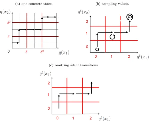
(a) one trace. (b) sampling values.
(c) omitting silent transitions.
Figure 4: Sampling values and omitting silent transitions along traces. Fig. 4(a) shows an example of a trace considering 2 chemical species A and B. The number of instances of the chemical species (denoted by the black lines) are sampled in intervals (represented by the red lines) (Fig. 4(b)). The transitions for which the number of instances remains in the same sampling interval (represented by the self-loops) are further ignored (Fig. 4(c)). The reactions associated with the transitions are here omitted.
Figure 6 shows the behaviour of the qualitative model refined with a mass in-variant for the case study with a race between a unary and a binary reaction, starting from the same initial states as in Figure 5.
The second kind of constraints that we consider consists in reasoning on the availability of resources in the system. Indeed when the number of instances of a chemical species enters a new sampling interval, there might not be enough resources in the system so that it may reach the next one. Figure 7 shows an example of such a situation for the case study of the model with an adaptor. Taking this kind of reasoning into account, we can suppress more unrealisable transitions, leading to a more accurate qualitative model. We show in Figure 8 the behaviour of the qualitative model after having discarded such unrealisable transitions from the model with a race between a unary and a binary reaction. The third kind of constraints that we consider comes from the separation between time scales. Unlike mass invariants and limiting resources, such con-straints do not emerge from the non deterministic semantics. Instead one has to refine the semantics in order to propose a way to model competitions be-tween reactions. First of all, one has to associate a quantity (according to the modelling paradigm, this may be a flux, a rate, a propensity, a priority level) with each reaction. In general, this quantity depends on the current state of the system (so as to take into account the amount of available reactants). Then, several options can be chosen according to the kind of modelling paradigms and to the kind of models that we consider.
reaction as a priority level, and in bounding the number of occurrences of lower priority reactions with respect to the number of occurrences of higher priority reactions, in each sequence of consecutive transitions.
(0,0,0) (0,0,1) 2 (0,1,0) 1 (0,0,2) 2 (0,1,1) 1 (0,1,2) 1 2 (0,2,0) 1 2 (0,2,1) 1 (0,2,2) 1 2 2 (1,0,0) 1,2 2 (1,0,1) 1 2 (1,1,0) 1 1,2 2 1 (1,0,2) 2 (1,1,1) 1 1,2 1 (1,1,2) 1 1,2 2 1 2 (1,2,0) 1 1,2 2 1 2 (1,2,1) 1 1,2 1 (1,2,2) 1 1,2 2 2 1,2 2 2 1,2 (2,0,0) 1,2 2 1 (2,0,1) 2 (2,1,0) 1 1,2 2 1 (2,0,2) 2 (2,1,1) 1 1,2 1 (2,1,2) 1 1,2 2 1 2 (2,2,0) 1 1,2 2 1 2 (2,2,1) 1 1,2 1 (2,2,2) 1 1,2 2 2 1,2 2 2 1,2
Figure 5: Behaviour of the qualitative model for the case study with a race between a unary and a binary reaction, starting from initial states with high levels of A and very low levels of B and C (node (2, 0, 0)). A node (n]A, n]B, n]C) represents a qualitative state for which the level of A, B and C is n]A, n]B and n]Crespectively. Arrows denote transitions resulting from the application of the reactions labelling the arrow. Reaction 1 denotes the unary reaction while reaction 2 denotes the binary one.
(0,0,0) (0,0,1) 2 (0,1,0) 1 (0,0,2) 2 (0,1,1) 1 (0,1,2) 1 2 (0,2,0) 1 2 (0,2,1) 1 (0,2,2) 1 2 2 (1,0,0) 1,2 2 (1,0,1) 1 2 (1,1,0) 1 1,2 2 1 (1,0,2) 2 (1,1,1) 1 1,2 1 (1,1,2) 1 1,2 2 1 2 (1,2,0) 1 1,2 2 1 2 (1,2,1) 1 1,2 1 (1,2,2) 1 1,2 2 2 1,2 2 2 1,2 (2,0,0) 1,2 2 1 (2,0,1) 2 (2,1,0) 1 1,2 2 1 (2,0,2) 2 (2,1,1) 1 1,2 1 (2,1,2) 1 1,2 2 1 2 (2,2,0) 1 1,2 2 1 2 (2,2,1) 1 1,2 1 (2,2,2) 1 1,2 2 2 1,2 2 2 1,2
Figure 6: Behaviour of the qualitative model for the case study of the race between a unary
and a binary reaction, refined with the mass invariant nA+ nB+ 2nC= AT, where nA, nB
and nCdenote the number of instances of A, B and C respectively, and starting from initial
states with high levels of A and very low levels of B and C (node (2, 0, 0)). The states that are discarded by the refinement are depicted in grey.
(a) (b)
Figure 7: Illustration of the limiting resource constraint for interval crossing on the case study of the model with an adaptor. (a) Petri Net represention of the adaptor model at the state
nA= 2, nB= 0, nC= 2, nAB= 2, nBC= 2 and nABC= 2, where nA, nB, nC, nAB, nBC
and nABC are the number of instances of the chemical species A, B, C, AB, BC and ABC
respectively. (b) Transition triggered after the application of the fourth reaction at the state indicated in Fig. 7(a). Black lines denote the number of instances of the chemical species whereas red ones represent the boundaries of the sampling intervals. The number of instances of ABC has just reached its next sampling interval after the occurrence of the fourth reaction. But now there is not enough resources of As and Cs so that the number of instances of ABCs reaches its next sampling interval.
Such an approach can be used to refine the constraints accounting for limiting resources, since not only there must be enough resources so that the number of instances of a given chemical species may reach a given sampling interval, but also a sampling interval should be reached through a trace in which low priority reactions are not used too often. When defining priorities in logical modelling [13], this execution assumption is pushed to the extreme case, that is to say that we assume that higher priority level reactions entirely preempt lower priority level ones. In our case studies, the results are robust: we obtain the same results using either one or the other assumption. Taking this kind of constraints into account in our approach leads to the suppression of the transitions forbidden by these constraints. Figure 9 shows the resulting qualitative model for the case study with a unary and a binary reaction, starting again from the same initial states as in Figure 6.
We applied our analysis refined with the three kinds of constraints to our case studies, using our prototype implementation to automatically derive qual-itative models with our approach [14]. The resulting models account for the properties of interest of our case studies. In particular, it is able to capture the sequestration e↵ect appearing in the model with adaptor. Figure 10 shows the behaviour of the qualitative model derived for this case study in the situation where we start from initial states with a very high level of B and low levels of A and C. Here we see that the level of ABC always remain very low, below
the initial level of A and C, therefore accounting for the sequestration e↵ect. A detailed analysis of the application of our approach to our case studies will be presented in Section 6. Before, in the following sections, we describe the formalisation of our approach.
(0,0,0) (0,0,1) 2 (0,1,0) 1 (0,0,2) 2 (0,1,1) 1 (0,1,2) 1 2 (0,2,0) 1 2 (0,2,1) 1 (0,2,2) 1 2 2 (1,0,0) 1,2 2 (1,0,1) 1 2 (1,1,0) 1 1,2 2 1 (1,0,2) 2 (1,1,1) 1 1,2 1 (1,1,2) 1 1,2 2 1 2 (1,2,0) 1 1,2 2 1 2 (1,2,1) 1 1,2 1 (1,2,2) 1 1,2 2 2 1,2 2 2 1,2 (2,0,0) 1,2 2 1 (2,0,1) 2 (2,1,0) 1 1,2 2 1 (2,0,2) 2 (2,1,1) 1 1,2 1 (2,1,2) 1 1,2 2 1 2 (2,2,0) 1 1,2 2 1 2 (2,2,1) 1 1,2 1 (2,2,2) 1 1,2 2 2 1,2 2 2 1,2
Figure 8: Behaviour of the qualitative model for the case study of the race between a unary and a binary reaction refined with the constraint of limiting resources for interval crossing, starting from initial states with high levels of A and very low levels of B and C (node (2,0,0)). A node (n]A, n]B, n]C) represents a qualitative state for which the level of A, B and C is n]A, n]B
and n]Crespectively. Arrows denote transitions resulting from the application of the reactions
labelling the arrow. Reaction 1 denotes the unary reaction whereas reaction 2 denotes the binary one. The transitions that can be discarded by the constraint of limiting resources are depicted in grey. (0,0,0) (0,0,1) 2 (0,1,0) 1 (0,0,2) 2 (0,1,1) 1 (0,1,2) 1 2 (0,2,0) 1 2 (0,2,1) 1 (0,2,2) 1 2 2 (1,0,0) 2 2 (1,0,1) 1 2 (1,1,0) 1 2 2 1 (1,0,2) 2 (1,1,1) 1 2 1 (1,1,2) 1 2 2 1 2 (1,2,0) 1 2 2 1 2 (1,2,1) 1 2 1 (1,2,2) 1 2 2 2 2 2 2 2 (2,0,0) 1,2 2 1 (2,0,1) 2 (2,1,0) 1 1,2 2 1 (2,0,2) 2 (2,1,1) 1 1,2 1 (2,1,2) 1 1,2 2 1 2 (2,2,0) 1 1,2 2 1 2 (2,2,1) 1 1,2 1 (2,2,2) 1 1,2 2 2 1,2 2 2 1,2
Figure 9: Behaviour of the qualitative model for the case study of a race between a unary and a binary reaction, refined with time scale separation, starting from initial states with high levels of A and very low levels of B and C (node (2,0,0)). The transitions discarded by the refinement are depicted in grey.
(0,4,0,2,2,0) (0,4,0,2,2,1) (0,4,1,2,2,0) (0,4,2,2,0,0) (0,4,2,2,1,0) (0,4,2,2,2,0) (1,4,0,2,2,0) (1,4,1,2,2,0) (1,4,2,2,0,0) (1,4,2,2,1,0) (1,4,2,2,2,0) (2,4,0,0,2,0) (2,4,0,1,2,0) (2,4,0,2,2,0) (2,4,1,0,2,0) (2,4,1,1,2,0) (2,4,1,2,2,0) (2,4,2,0,0,0) (2,4,2,0,1,0) (2,4,2,1,0,0) (2,4,2,0,2,0) (2,4,2,1,1,0) (2,4,2,1,2,0) (2,4,2,2,0,0) (2,4,2,2,1,0) (2,4,2,2,2,0) (0,4,0,2,2,2)
Figure 10: Behaviour of the qualitative model refined with the three kinds of constraints (the mass invariants, the limiting resources for interval crossing and time scale separation) for the case study of the model with an adaptor, starting from initial states with very high levels of B, low levels of A and C and very low levels of AB, BC and ABC (node (2,4,2,0,0,0)), under the modelling assumptions stated in Section 6. A node (n]A, n]B, n]C, n]AB, n]BC, n]ABC) represents a qualitative state for which the level of A, B, C, AB, BC and ABC is n]A, n]B, n]C, n]AB,
n]BC and n]ABC respectively. Arrows denote single or multiple transitions. The reactions
associated with the transitions are omitted. The transitions discarded by the constraint of limiting resources on interval crossing are depicted in grey.
3. Trace semantics
We want to design a framework to automatically abstract qualitative mod-els from reaction networks. Following a formal approach, we will relate the behaviour of the abstract model with the behaviour of the reaction network. Thus, the first task is to provide a formal definition for the behaviour of reac-tion networks. In this secreac-tion, we describe this behaviour qualitatively in terms of a set of traces. Partial information about reaction kinetics will be taken into account in Section 5.3.
Firstly, we give the definition of a reaction network.
Definition 1 (Reaction network). A network R of n reactions is a pair ⇣
⌫, (Mr, Vr)1rn
⌘
(1) ⌫ is a set of chemical species; (2) for each integer r between 1 and n:
(a) Mr: ⌫ ! N is a multi-set of chemical species,
(b) Vr: ⌫ ! Z is a reaction vector,
such that Mr(x) + Vr(x) 0 for any chemical species x2 ⌫.
In Definition 1, a pair (Mr, Vr) is called a reaction. In a reaction (Mr, Vr), the
multi-set Mrencodes the set of the reactants (with their multiplicities) whereas
the vector Vr denotes how many chemical species of each kind is produced and
consumed at each application of the reaction. Lastly, for each chemical species x2 ⌫, the following constraint:
Mr(x) + Vr(x) 0,
ensures that the reaction r does not consume more instances of the chemical species x than available in the system. A list of symbols used in the text with their description is provided in Table 1.
Example 1. Let us illustrate our definition of a reaction network on the case study with a competition between a unary reaction and a binary reaction (Sec-tion 2):
A !B
2A !C
Three chemical species A, B and C compose this system. Thus the set of chemical species is ⌫ ={A, B, C}. The set of reactants of the unary reaction is reduced to A with a multiplicity of 1. The associated multiset M1 is thus:
M1 : 8 > < > : A7! 1, B7! 0, C7! 0.
The result of the application of the unary reaction is the consumption of 1 in-stance of A and the production of 1 inin-stance of B. The associated reaction vector V1 is thus: V1 : 8 > < > : A7! 1, B 7! 1, C7! 0.
Considering the binary reaction, its set of reactants is A with a multiplicity of 2. The associated multiset M2 is thus:
M2 : 8 > < > : A7! 2, B7! 0, C7! 0.
The result of the application of the binary reaction is the consumption of 2 instances of A and the production of 1 instance of C. The associated reaction vector V2 is thus: V2 : 8 > < > : A7! 2, B 7! 0, C7! 1.
We can now formally define the set of transitions of a reaction network. Definition 2 (Transition system). A reaction network R induces a transi-tion system (QR, TR) where:
(i) QRis the set N⌫ of the functions between ⌫ andN;
(ii) TR is the subset of N⌫⇥ J1, nK ⇥ N⌫ that contains all the triple (q, r, q0)
such that, for all chemical species x2 ⌫: (a) Mr(x) q(x) and
(b) q0(x) = q(x) + Vr(x),
where R =⇣⌫, (Mr, Vr)1rn
⌘ .
In Definition 2, the notation J1, nK denotes the set of the integers between 1 and n. The set QR denotes all the potential states of the system. At this
level of abstraction, the state of the system describes the number of instances of each kind of chemical species. The elements of TR are called the transitions
of the system. Transitions define the result of the applications of reactions. More precisely, a triple (q, r, q0)2 T
Rdenotes the fact that the system can jump
from the state q to the state q0 by applying the rule indexed by the integer r.
Condition (iia) ensures that enough reactants are available, whereas condition (iib) encodes the consumption/production of the chemical species. We notice that the resulting transition system is equivalent to a Petri net [12], in which each kind of chemical species is denoted by a placeholder and each instance by a token.
Before defining the traces of a reaction network, we introduce some notations.
For any two sets A and ⌃, and any subset T of the set A⇥ ⌃ ⇥ A, we call a
pretrace of elements of A and transitions in T , any element of the set A⇥ T?.
In a pretrace:
⌧ =⇣a00, (ai, i, a0i)1ik
⌘ , the element a0
0 (resp. a0k) is called the initial (resp. final) state of the pretrace ⌧
and is denoted as first(⌧ ) (resp. final(⌧ )). The second component of a pretrace is a (potentially empty) sequence of triples in T . Moreover, the pretrace ⌧ is called a trace if ai = a0i 1 for any integer i between 1 and k. Lastly, given a
triple (ak+1, k+1, a0k+1) in T , we denote by:
⌧ a (ak+1, k+1, a0k+1)
the following pretrace: ⇣
a00, (ai, i, a0i)1ik+1
⌘ ,
that is obtained by adding the transition (ak+1, k+1, a0k1) at the end of the
pretrace ⌧ .
We can now properly define the trace semantics of a reaction network. Definition 3 (Trace semantics). The set of traces that is induced by a re-action network R and a set of initial states QR,0✓ QR is defined as the set of
the traces ⌧ of elements of QR and transitions in TR such that first(⌧ )2 QR,0.
We denote byTR,QR,0the set of traces that is induced by the reaction network
R and the set of the initial statesQR,0.
Example 2. Figure 3 illustrates the notion of trace semantics on the model with the adaptor (Section 2). Figure 3(a) shows the Petri net representation of the reaction network of the model for the set of initial states QR,0={q}, where
the state q is defined as follows:
q : 8 > > > > > > > > < > > > > > > > > : A 7! 2, B 7! 1, C 7! 2, AB 7! 0, BC 7! 0, ABC 7! 0.
Figure 3(b) displays the induced transition system. Starting from the initial state, reaction 1 (resp. reaction 2) can occur giving rise to a transition resulting in the consumption of 1 instance of A and B (resp. 1 instance of B and C) and the production of 1 instance of AB (resp. BC). Reaction 3 (resp. reaction 4) can then be instantiated giving rise to a transition resulting in the consumption of 1 instance of AB and C (resp. 1 instance of A and BC) and the production of 1 instance of ABC. No reaction can then occur as there are not enough reactants available.
Altogether the traces that are induced by the reaction network and the initial state are: (2, 1, 2, 0, 0, 0), (2, 1, 2, 0, 0, 0) 1! (1, 0, 2, 1, 0, 0), (2, 1, 2, 0, 0, 0) 2! (2, 0, 1, 0, 1, 0), (2, 1, 2, 0, 0, 0) 1! (1, 0, 2, 1, 0, 0) 3! (1, 0, 1, 0, 0, 1), (2, 1, 2, 0, 0, 0) 2! (2, 0, 1, 0, 1, 0) 4! (1, 0, 1, 0, 0, 1),
where a state q is denoted by the sextuple (q(A), q(B), q(C), q(AB), q(BC), q(ABC)) and a transition (q, r, q0) as q r! q0.
Following the abstract interpretation framework [15], we can also express the trace semantics as the least fixpoint of a monotonic function over the powerset of pretraces }(QR⇥ TR?). Let FQR,0 be the following function:
FQR,0 :
(
}(QR⇥ TR?)! }(QR⇥ TR?)
Roughly speaking, the function FQR,0 maps any set of pretraces X to the set
of pretraces that can be obtained by continuing a pretrace in the set X with a transition in TR. We notice that the function FQR,0 is a monotonic function,
that is to say that:
X✓ Y ) FQR,0(X)✓ FQR,0(Y ).
Since additionally the function FQR,0 is defined over a powerset, it has a least
fixpoint [16]. This least fixpoint, lfpFQR,0, is indeed the set of all the traces of
the reaction network R, that is to say that: lfpFQR,0=TR,QR,0.
Moreover, the functionFQR,0 is[-continuous, that is to say that:
FQR,0
⇣[
{Xj | j 2 J}
⌘
=[{FQR,0(Xj)| j 2 J}
for any family (Xj)j2J of sets of pretraces. It follows from [17] that the least
fixpoint ofFQR,0 can also be expressed as the limit of the finite iterates of the
functionFQR,0, that is to say that:
TR,QR,0 =
[
{FiQR,0(;) | i 2 N},
which provides an iterative algorithm to enumerate the traces of the network R.
4. Derivation of a coarse-grained qualitative semantics
The semantics described in Section 3 is too fine grained. In particular, each instance of a protein is taken into account. Usually, in a qualitative model, the number of instances of proteins is sampled within a finite number of intervals. In this section, we will use the abstract interpretation framework to derive such an abstraction. Abstract interpretation [15] is a unifying framework for the approximation of mathematical structures. It o↵ers formal tools to relate the observations of the behaviour of a system at di↵erent levels of details. It can also be used to systematically derive static analysers (that provide e↵ective definitions of semantics at coarser levels of abstraction).
We use a simple version of the abstract interpretation framework that con-sists in removing some information from values, states and traces. Our abstrac-tion is twofold. Firstly, we sample the number of instances of chemical species within a finite number of intervals. Secondly, we remove in traces the transitions for which the number of instances of each chemical species remains in the same interval. To sample the number of instances and later the rate of reactions (see Section 5.3), we partition the set R+ over the p + 1 intervals J0, J, J i, i+1J
for each integer i between 1 and p 1, andJ p,
1J, where p and are integer
parameters such that 2 and p 1.
We introduce a function R to sample non-negative real numbers over this partition:
(a) concrete states. (b) abstract states.
Figure 11: Abstraction of values. The domain of states (hereR2) is partitioned by intervals
(represented by the red lines) following a geometric progression, parametrised by (Fig.
11(a)). The number of instances (denoted by the black lines) in each interval is then abstracted away and the intervals are mapped to their corresponding abstract values (Fig. 11(b)).
Definition 4 (abstract values). We define the function R between the set
R+ and the setJ0, pK as follows: R : ( R+ ! J0, pK v 7! min {p} [ {k 2 J0, pK | v < k+1 } .
This way, the function Rmaps each positive real number v 2 R+ into the
least integer in the set{p}[{k 2 J0, pK | v < k+1}. This abstraction is depicted
in Figure 11.
Then we lift the function Rover transition systems.
Definition 5 (abstract transition system). A reaction network R induces an abstract transition system (Q]R, TR]) where:
(i) Q]Ris the setJ0, pK⌫of the functions between the set of the chemical species
⌫ and the integer intervalJ0, pK;
(ii) TR] is the subset ofJ0, pK⌫⇥J1, nK⇥J0, pK⌫that is defined by (q], r, q]0)2 T] R
if and only if there exist (q, r, q0)2 TR such that:
q]= R q and q]0= R q0.
Thus, the abstract transition system is obtained by applying component-wise the function Rin the states of the transition system and in the states that occur in transitions. We denote by Qthe following function:
Q :
(
QR! Q]R
q 7! R q.
The function Qmaps each state q2 Q
Rinto the abstract state R q2 Q]Rby
applying the abstraction function Rcomponent-wise on the number of instances of each species.
Then the abstraction Q can be lifted to pretraces and traces. We call an
of Q]R and transitions in TR]. We denote by T
1 the function between the set
QR⇥ TR? and the setQ ] R⇥ T
]?
R that is defined as follows: T 1 : ( QR⇥ TR? ! Q ] R⇥ T ]? R ⇣ q0 0, (qi, ri, q0i)1ik ⌘ 7!⇣ Q(q0 0), Q(qi), ri, Q(qi0) 1ik ⌘ .
Roughly speaking, the function 1T applies the abstraction function Q over
each state that occurs in a trace (or a pretrace).
We notice that there exists some abstract transitions (q], r, q]0)2 T] R such
that q] = q]0. Indeed, even if a concrete transition changes the number of
instances of a chemical species, this does not always make it exit its sampling interval. We call such transitions silent and we denote by TR/"] the set of the non silent abstract transitions. In order to remove silent transitions, we define
the function T
2 between the setQ
] R⇥ T
]?
R and the setQ
] R⇥ T ]? R/"as follows: T 2 : ( Q]R⇥ T ]? R ! Q ] R⇥ T ]? R/" ⇣ q0]0, ⇣ qi], ri, q]i0 ⌘⌘ 7!⇣q]00, ⇣
q](i), r (i), q]0(i)
⌘⌘ , where (i) ranges over the set {i 2 J1, kK | qi] 6= q
]
i0} in increasing order. We
notice that the function T
2 removes the transitions between identical abstract
states from abstract pretraces.
Example 3. Figure 12 shows an illustration of the application of the functions
T
1 and 2T, in a 2-dimensional case (considering 2 chemical species x1 and
x2), on the abstraction of the following concrete trace (for which we omit the
reactions for sake of clarity):
⌧ = (0, 1) ! (1, 1) ! (1, 3) ! (2, 3) ! (3, 3)
! (4, 3) ! (4, 5) ! (5, 5) ! (6, 5)
where we denote a state q by the couple (q(x1), q(x2)) (see Fig.12(a)). Here we
assume that = 2. Abstracting first the states of the transitions composing the trace (by applying the function T1 to the trace), we get:
T
1(⌧ ) = (0, 0) ! (0, 0) ! (0, 1) ! (1, 1) ! (1, 1)
! (2, 1) ! (2, 2) ! (2, 2) ! (2, 2). where we denote an abstract state q] by the couple (q](x
1), q](x2)) (see Fig.
12(b)). Removing then the silent abstract transitions (by applying the function
T
2), we get: T
2( 1T(⌧ )) = (0, 0) ! (0, 1) ! (1, 1) ! (2, 1) ! (2, 2).
(see Fig. 12(c)).
Now we are ready to define our abstraction function over traces. We intro-duce the function T between the set of concrete (pre)tracesQR⇥ TR? and the
set of abstract (pre)traces Q]R⇥ T ]? R/"as follows: T : ( QR⇥ TR?! Q ] R⇥ T ]? R/" ⌧ 7! 2T( 1T(⌧ )).
(a) one concrete trace. (b) sampling values.
(c) omitting silent transitions.
Figure 12: Abstraction of traces. Fig. 12(a) shows an example of a concrete trace in a
2-dimensional case (i.e. considering 2 chemical species x1 and x2). We here assume = 2.
Following the abstraction of values, the domain of values is partitioned by intervals (repre-sented by the red lines) and the number of instances (denoted by the black lines) in each interval is abstracted away. The states of the transitions composing a trace are then mapped to their corresponding abstract states (Fig. 12(b)). Finally the transitions which have no e↵ect on the abstract states (represented by the self-loops) are removed from the trace (Fig. 12(c)). The reactions associated to the transitions are here omitted.
Indeed, the function T is the composition of the functions T2 and 1T.
The function T can be used to abstract the computation of the trace se-mantics. Given a set of initial states QR,0 ✓ QR, we introduce the function
F]
QR,0 over the powerset of abstract (pre)traces }(Q
] R⇥ T ]? R/") as follows: F] QR,0 : ( }(Q]R⇥ T ]? R/")! }(Q ] R⇥ T ]? R/") Y 7! ↵T F QR,0 T(Y ) , where:
(i) the function ↵T is defined as follows:
↵T : ( }(QR⇥ TR?)! }(Q ] R⇥ T ]? R/") X 7! { T(x)2 Q] R⇥ T ]? R/"| x 2 X}; ;
(ii) the function T is defined as follows:
T : ( }(Q]R⇥ T ]? R/")! }(QR⇥ TR?) Y 7! {x 2 QR⇥ TR? | T(x)2 Y }.
(see p.15 for a definition of the functionFQR,0). Roughly speaking the function
↵T maps each set of concrete (pre)traces to the set of their abstractions. This
is, indeed, the best abstraction of a set of traces with respect to our abstraction
T over (pre)traces. Conversely, the function T maps each set of abstract
(pre)traces to the set of the concrete traces which can be abstracted into one of these abstract traces. Given a subset of concrete (pre)traces X ✓ QR⇥ TR?
and a subset of abstract (pre)traces Y ✓ Q]R⇥ TR/"]? , the property ↵T(X)✓ Y
is equivalent to the property X ✓ T(Y ). Such a pair of functions is called a
Galois connection [15], which is usually denoted as follows:
}(QR⇥ TR?) !
↵T
T
}(Q]R⇥ TR/"]? ).
A Galois connection ensures that each set of concrete elements (here concrete (pre)traces) has a best abstraction in the abstract. Moreover, it ensures that
the function ↵T F
QR,0 T is the most precise counterpart to the function
FQR,0, that is to say that:
(1) for each set Y 2 }(Q]R⇥ TR/"]? ) of sets of abstract (pre)traces, we have: FQR,0(
T(Y ))✓ T(F]
QR,0(Y ));
(2) and for any function G over the set }(Q]R⇥ T ]?
R/") of sets of abstract
(pre)traces such that:
FQR,0( T(Y ))✓ T(G(Y )),
for each set Y 2 }(Q]R⇥ TR/"]? ), we have: F]
QR,0(Y )✓ G(Y ),
for each set Y 2 }(Q]R⇥ TR/"]? ).
We define the Galois connections (↵R, R) (resp. (↵Q, Q)) between sets of concrete values (resp. states) and sets of abstract values (resp. states) the same way.
The functionF]QR,0 is monotonic. Thus, by [16], it has a least fixpoint. Definition 6 (abstract trace semantics). The set of abstract traces TQ]R,0
that is induced by a reaction network R and a set of initial states QR,0✓ QR
is defined as the least fixpoint lfpF]QR,0 of the functionF]QR,0.
The Galois connection (↵T, T) can be used to transfer the computation of
the concrete fixpointTR,QR,0 = lfpFQR,0 in the abstract.
Theorem 1 (fixpoint transfer). Let R be a reaction network andQR,0✓ QR
a set of initial states.
Then the set lfpFQR,0 is a subset of the set T(lfpF
] QR,0).
We have used the Galois connection (↵T, T) so as to abstract the trace
se-mantics. Theorem 1 ensures that our abstraction is conservative, i.e. all the traces of the concrete semantics are taken into account. Moreover, the set of abstract traces can be computed by iterating the function ↵T F
QR,0 T. This
consists in, at each step, (a) computing the concretization of the set of traces, (b) making the computation in the concrete, and (c) abstract the result.
The following property provides a direct way to make this computation with-out going back and forth in the concrete, and gives more intuition abwith-out what information is lost with our abstraction. We introduce the following notations:
• we denote by V1( resp. M1) the greatest element among the set{|Vi(x)| | i 2
J1, nK, x 2 ⌫} (resp. among the set {Mi(x)| i 2 J1, nK, x 2 ⌫}), and
de-note by (M +V )1the greatest element among the set{|Mi(x)+Vi(x)| | i 2
J1, nK, x 2 ⌫};
• for any integer z 2 Z, we define the sign sign(z) of z as: (1) sign(0) = 0, and
(2) sign(z) = z/|z| if z 6= 0;
• for any function f between two sets A and B and any elements y 2 A and v2 B, we define f[y 7! v] as the function between A and B mapping the element y to the element v, and any element x2 A \ {y} to the element f (x).
Property 1. The following assertions hold:
(1) For any part Y ✓ Q]R⇥ TR/"]? , the following inclusion:
F] QR,0(Y )✓ Y [ ↵ Q(Q R,0)[ 8 < :⌧ ]a (q], r, q]0) ⌧] 2 Y ^ (q], r, q]0)2 T] R/" ^ final(⌧]) = q] 9 = ;, is satisfied.
(2) If for any concrete transition (q, r, q0)2 T
R such that ( Q(q), r, Q(q0))2
TR/"] , there exist a state q00 and a reaction r0 such that (q00, r0, q) 2 TR
and Q(q00) = Q(q), then for any part Y ✓ Q] R⇥ T ]? R/", the following inclusion: ↵Q(QR,0)[ 8 < :⌧ ]a (q], r, q]0) ⌧]2 Y ^ (q], r, q]0)2 T] R/" ^ final(⌧]) = q] 9 = ;✓ F ] QR,0(Y ), is satisfied.
(3) For any abstract transition (q], r, q]0) 2 T]
R, if > V1, then the value
q]0(x) is either equal to q](x) or to q](x) + sign(V r(x)).
(4) For any rule r and any abstract state q]
2 Q]R, if > max(M1, (M +
V )1), then, for any chemical species y 2 ⌫ such that Vr(y) 6= 0 and
0 q](y) + sign(V
r(y)) p, we have:
(q], r, q][y 7! q](y) + sign(V
Properties 1.(1) and 1.(2) provide an inductive definition to compute the set of the abstract traces directly, without having to concretize the states. More precisely, Property 1.(1) proposes a sound over-approximation of the function F]
QR,0, that can be directly computed in the abstract domain. Moreover, in
Property 1.(2), this abstraction is shown to be complete.
It is worth noting that the inclusion in Property 1.(1) would not have hold in general if we had not taken the extensive closure of the abstract function (the extensive closure of a function f over the subsets of a given set A, is the least function (component-wise) that is extensive and greater (component-wise) than the function f ; indeed the extensive closure of a function f is always mapping
each subset X ⇢ A, to the subset X [ f(X)). Replacing a function by its
extensive closure is not an issue, since a given function and its extensive closure have the same set of fixpoints [18].
Property 1.(2) shows that this abstraction is complete (that is to say that it introduces no spurious behaviour), under the assumption that for any concrete transition ⌧ such that its abstraction is not silent, there exists a concrete tran-sition ⌧0 that is silent in the abstract and which final state is the initial state of
⌧ . This assumption models the fact that we ignore the di↵erence between two states having the same abstraction. It is satisfied, if the parameter is chosen large enough, or if we add a spurious reaction r with no reactant and no product in the system.
Property 1.(3) establishes the fact that it is not possible to cross a whole interval in a single transition. As formalised in Theorem 1, the abstract trace semantics is a safe over-approximation of the concrete trace semantics. Yet, this semantics introduces spurious behaviours. In particular, Property 1.(4) establishes that it is always possible to change the interval of a chemical species x2 ⌫ in the direction given by the sign of Vr(x), when applying the rule that is
indexed with the integer r, unless the chemical species x 2 ⌫ is already in the first or in the last interval of the partition.
In the present form, our abstraction is not precise enough to capture the properties of interest of our case studies (Section 2). In particular the sequestra-tion e↵ect, which appears in the adaptor model, is not captured in the abstract semantics. Indeed, following Property 1.(4), it is always possible to increase the abstract level of the trimer ABC along a trace, whatever the initial concentra-tion of B, until its level reaches its maximum value. Thus we cannot conclude from our abstract system that high levels of the adaptor protein B prevents the formation of ABC in the concrete one.
Example 4. Figure 5 gives an illustration of the abstract transition system for the second case study (Section 2):
A !B
2A !C
starting from any initial state q 2 QR such that Q(q) satisfies the following
constraints: 8 > < > : Q(q)(A) = 2, Q(q)(B) = 0, Q(q)(C) = 0.
Here we assume > 2 (which ensures that > max(M1, (M + V )1) and thus that Prop. 1.(4) applies) and p = 2. Again following Property 1.(4), it is always possible to increase the abstract level of B and C until they reach their maximum levels. Thus we cannot conclude from our abstract system that, in the concrete one, a competition between the production of B and the production C occurs depending on the initial concentration of A.
We will refine our abstraction in the next section in order to capture the properties of interest of our case studies.
5. Refinements
As we have noticed in Section 4, the abstraction TQ]R,0 is very coarse. In particular, it does not exploit the following three kinds of situations. Firstly, the number of instances of chemical species may be entangled by some mass preservation invariants. Secondly, when the number of instances of a chemical species enters a new interval, it is sometimes possible to prove that there are not enough resources in the system to make this number reach the next interval. Thirdly, our concrete semantics is purely qualitative. We propose to add kinetic rates and abstract them accurately in order to account for the potential races between reactions.
In this section, we propose three refinements of the abstract semantics to formalise three corresponding classes of reasoning. These refinements are or-thogonal: they can be combined by the means of a reduced product [15]. 5.1. Mass invariants
5.1.1. Inference
In the concrete semantics, the number of instances of the chemical species may be related by some mass conservation equations.
Example 5. Back to the example of Figure 3, the states composing the set of traces induced by the reaction network of the adaptor model and the initial state (2, 1, 2, 0, 0, 0) are:
(2, 1, 2, 0, 0, 0), (1, 0, 2, 1, 0, 0), (2, 0, 1, 0, 1, 0), (1, 0, 1, 0, 0, 1).
where each state q is denoted as the following sextuple: (q(A), q(B), q(C), q(AB), q(BC), q(ABC)).
Thus, along this set of traces, the number of instances of As remains constant equal to 2, that is to say that:
q(A) + q(AB) + q(ABC) = 2,
the number of instances of Bs remains constant equal to 1, that is to say that: q(B) + q(AB) + q(BC) + q(ABC) = 1,
and the number of instances of Cs remains constant equal to 2, that is to say that:
In general, mass invariants are numerical constraints of the following form: X
↵xq(x) = b
for (↵x)x2⌫2 N⌫ and b2 N (i.e. semi-positive constraints).
Several solutions to obtain the semi-positive constraints that are satisfied in a network are available in the literature [19, 20, 21].
Without further information about the composition of chemical species, one solution consists in combining the vectors of a basis of the smallest affine space affine hull(R,QR,0) that contains all the states that are reachable in zero, one,
or several computation steps (from one initial state in QR,0) in the reaction
network R, in order to form constraints with non-negative coefficients only and remove the constraints in which negative coefficients cannot be eliminated. The affine hull affine hull(R,QR,0) is indeed the smallest affine set that contains the
initial states and that is close with respect to each reaction vector, that is to say that: affine hull⇣⇣⌫, (Mr, Vr)1rn ⌘ ,QR,0 ⌘ =\ 8 > > < > > : E✓ QR E is an affine set QR,0✓ E 8~u 2 E, 8i 2 J1, nK, ~u + Vi2 E 9 > > = > > ; .
Example 6. Keeping on with the example of Figure 3, we start with the affine set that contains the unique initial state. This set is defined as the solutions of the following set of affine equations:
S0 : 8 > > > > > > > > < > > > > > > > > : q(A) = 2, q(B) = 1, q(C) = 2, q(AB) = 0, q(BC) = 0, q(ABC) = 0.
The solution of the set of equations S0 is not close with respect to the reaction
vector of the first reaction:
V10 : 8 > > > > > > > > < > > > > > > > > : A 7! 1, B 7! 1, C 7! 0, AB 7! 1, BC 7! 0, ABC 7! 0.
The smallest affine set containing the solution of S0 and that is close with
respect to the vector V10 is defined as the solutions of the following set of affine
equations: S1 : 8 > > > > > > < > > > > > > : q(A) + q(AB) = 2, q(B) + q(AB) = 1, q(C) = 2, q(BC) = 0, q(ABC) = 0.
The solution of the set of equations S1 is not close with respect to the reaction
vector of the second reaction:
V20 : 8 > > > > > > > > < > > > > > > > > : A 7! 0, B 7! 1, C 7! 1, AB 7! 0, BC 7! 1, ABC 7! 0.
The smallest affine set containing the solution of S1 and that is close with
respect to the vector V20 is defined as the solutions of the following set of affine
equations: S2 : 8 > > > < > > > : q(A) + q(AB) = 2, q(B) + q(AB) + q(BC) = 1, q(C) + q(BC) = 2, q(ABC) = 0.
The solution of the set of equations S2 is not close with respect to the reaction
vector of the third reaction:
V30 : 8 > > > > > > > > < > > > > > > > > : A 7! 0, B 7! 0, C 7! 1, AB 7! 1, BC 7! 0, ABC 7! 1.
The smallest affine set containing the solution of S2 and that is close with
respect to the vector V0
3 is defined as the solutions of the following set of affine
equations: S3 : 8 > < > :
q(A) + q(AB) + q(ABC) = 2,
q(B) + q(AB) + q(BC) + q(ABC) = 1, q(C) + q(BC) + q(ABC) = 2,
The solution of the set of equationsS3is close with respect to the reaction vector
of the fourth reaction:
V40 : 8 > > > > > > > > < > > > > > > > > : A 7! 1, B 7! 0, C 7! 0, AB 7! 0, BC 7! 1, ABC 7! 1. .
A basis for the smallest affine set that contains the initial state and that is close with respect to each reaction vector can be computed by using Gaussian
elimination at a time complexity O(n(m + n)3) and at a memory complexity
O(mn) [19] (where m denotes the number of chemical species, that is to say the cardinal of the set ⌫, and n represents the number of reactions).
Getting a basis of the semi-positive invariants is more difficult, since there exist networks which possess an exponential number of minimal semi-positive invariants. A complete solution is proposed in [21]. In [20], a heuristics is used to drive the computation and get a subset of the semi-positive invariants at a
time complexity O(n(m + n)3) and a memory complexity O(mn).
Example 7. Keeping on with the example of Figure 3, we notice that the system S3 contains only non-negative coefficients. Thus it is already composed of
semi-positive constraints.
When the composition of chemical species is known, one can use them as a hint to discover quickly potential semi-positive invariants. Assume that we are
given a set CU of chemical units and a function comp mapping each chemical
species x2 ⌫ into a multi-set NCU of chemical units. Given a chemical species
x2 ⌫ and a chemical unit cu 2 CU, we denote by comp(x)(cu) the number of
occurrences of the chemical unit cu in the multi-set comp(x), and we assume that this is actually the number of instances of the chemical unit cu in the chemical species x.
The overall number of a chemical unit cu2 CU in a given state q 2 QR, can
be expressed as the following linear combination: X
{comp(x)(cu)q(x) | x 2 ⌫}.
Moreover, this is a semi-positive invariant if and only if it is preserved by each reaction, that is to say, if for each i2 J1, nK, the following:
X
{comp(x)(cu)V (x) | x 2 ⌫} = 0 is satisfied.
As a consequence, detecting which proteins are preserved by a set of reactions
can be done at time complexity O(mm0n) (where m0 denotes the number of
chemical units, that is to say the cardinal of the setCU).
Example 8. Keeping on with the example of Figure 3, we assume that chem-ical species are made of three kinds of proteins, A, B, and C, and that the composition of chemical species is given in tabular form as follows:
A B C A 1 0 0 B 0 1 0 C 0 0 1 AB 1 1 0 BC 0 1 1 ABC 1 1 1
Thus, in a given state q2 QR, the overall number of instances of protein A is
given by the following semi-positive linear form: q(A) + q(AB) + q(ABC);
the overall number of instances of protein B is given by the following semi-positive linear form:
q(B) + q(AB) + q(BC) + q(ABC);
and the overall number of instances of protein C is given by the following semi-positive linear form:
q(C) + q(BC) + q(ABC).
Moreover, each of these linear forms is orthogonal to each reaction vector of the reaction network, that is to say that the result of the application of any of these three linear forms to any of the four reaction vectors is equal to 0. Thus they induce semi-positive invariants for the system.
5.1.2. Analysis refinement
Mass preservation invariants are particular cases of trace invariants and can thus be used to refine our abstraction. Let inv✓ QR⇥ TR? be a trace invariant.
Formally, this means that:
FQR,0(inv)✓ inv.
(see p.15 for a definition of the functionFQR,0). By [16], the concrete semantics
is the most precise of the trace invariants, that is to say that: TR,QR,0 =
\
{X | FQR,0(X)✓ X}.
In particular,TR,QR,0✓ inv. It follows that:
lfpFQR,0 = lfpF
INV QR,0,inv,
where the function FINV
QR,0,invis defined as follows:
FINV QR,0,inv :
(
}(QR⇥ TR?)! }(QR⇥ TR?)
X 7! FQR,0(X)\ inv.
Here the function FINV
QR,0,inv maps any set of pretraces X ✓ QR⇥ T
? R to the
intersection between the set FQR,0(X) and the trace invariant inv. The least
fixpoints of both functions FQR,0 and F
INV
QR,0,inv are equal, but the abstraction
of the iterates of the latter may be more precise. LetFINV]QR,0,inv be the function that is defined as follows:
FINV] QR,0,inv : ( }(Q]R⇥ T ]? R/")! }(Q ] R⇥ T ]? R/") Y 7! ↵T ⇣FINV QR,0,inv T ⌘.
(see p.19 for a definition of the Galois connection (↵T, T)). The function ↵T
is\-complete, so the function FINV]QR,0,inv is equal to:
[Y 7! F]QR,0(Y )\ ↵T(inv)].
The iterates of the functionFINV]QR,0,invprovide another e↵ective way, more precise but still sound, to abstract the trace semantics:
Theorem 2 (abstract trace semantics with invariants). LetQ0
R,0be a
sub-set ofQR,0 and inv be a part ofTR,QR,0 such thatFQ0R,0(inv)✓ inv.
Then, we have: TR,Q0 R,0 ✓ T(lfp [Y 7! F] Q0 R,0(Y )\ ↵ T(inv)]).
In Theorem 2, we have partitioned the traces to separate the computation of their abstraction according to their initial states (for more details about trace partitioning, see [22, 23]). This leads to a more accurate abstraction whenever some pairs of initial states do not share the same invariants.
When the trace invariant is a set of semi-positive constraints, the following property gives an explicit definition for the term ↵T(inv).
Property 2 (mass invariant separation). Let:
• (ax)x2⌫ 2 N⌫\ {0}⌫ be a family of positive integer coefficients (with at
least one not equal to 0),
• b 2 N be a non-negative integer coefficient,
• S be the sum of the coefficients ax for all chemical species x2 ⌫ (i.e.
S =Px2⌫ax),
• for any abstract state q], q]
max be the maximum element of the following
set:
{k 2 J0, pK | 9x 2 ⌫, ax> 0 ^ k = q](x)}.
If b S R(b), the following set:
↵Q ( q2 QR b = X x2⌫ axq(x) )!
is equal to the following set: {q]
2 Q]R| q ]
max= R(b)}.
Otherwise, it is a subset of the following set: ⇢ q]2 Q]R R(b) ⇠ S⇡ q] max R(b) .
Proof of Property 2 is given in Appendix A.2.
Property 2 has a flavour of tropical algebræ [5]. In particular, whenever the affine constants of mass preservation invariants are far enough from the lower bound of their sampling interval, the abstraction of the number of instances of a protein is equal to the abstraction of the number of instances of the most abundant chemical species containing this protein. Otherwise, if the parameter
is chosen great enough (that is to say that S), Property 2 still ensures
that the abstraction of the number of instances of a protein is either the same as the abstraction of the number of instances of the most abundant chemical species containing this protein, or the next one.
Figure 13: Illustration of mass invariant separation on the case study of the adaptor model, taking as mass invariant the preservation of the overall number of As: q(A) + q(AB) +
q(ABC) = AT. We assume = 4 and v(AT) = 1 (i.e. 4 AT < 16). Blue lines
de-note the threshold S v(AT)= 12. If AT 12, the abstraction of the mass invariant is the
set of states q]such that max(q](A), q](AB), q](ABC)) = 1. Otherwise it is the set of states
q]such that max(q](A), q](AB), q](ABC))2 {0, 1} (Prop. 2).
Example 9. Figure 13 shows an illustration of the application of Property 2 on the case study of the adaptor model, taking as mass invariant the preservation of the overall number of As:
q(A) + q(AB) + q(ABC) = AT.
We assume that = 4 and v(A
T) = 1 (i.e. the affine constant AT belongs to
the sampling interval J , 2J). The sum of the coefficients of the mass equation
is S = 3. Thus we have > S and S v(AT)= 12 (depicted by the blue lines in
Fig. 13).
Therefore, following Property 2, if AT 12, the abstraction of the mass
invariant is the set of states q] such that:
max(q](A), q](AB), q](ABC)) = 1. Otherwise it is the set of states q] such that:
max(q](A), q](AB), q](ABC))
2 {0, 1}.
Example 10. Figure 6 gives an illustration of the induced set of abstract tran-sitions for the case study of the model showing a race between a unary and a binary reaction:
A !B
2A !C
refined with the following mass invariant:
and starting from the same initial state as in Figure 5, i.e. starting from any initial state q2 QR such that Q(q) satisfies the following constraints:
Q(q) : 8 > < > : A7! 2, B 7! 0, C7! 0.
Here we assume that p = 2, > 4 and that the affine constant AT is far from
the lower bound of its sampling interval (AT = 4 2). Following Property 2, the
abstraction of the mass invariant is thus the set of states q] such that:
max(q](A), q](B), q](C)) = 2
(depicted by the black nodes in Fig. 6). By soundness of the abstraction (Thm. 2), we can thus conclude from our abstract semantics that, in the concrete one, the number of instances of A will not decrease below 2 before either the number of
instances of B or the number of instances of C exceeds 2.
5.2. Watching interval boundaries
So far, we have approximated the number of instances of each chemical species by means of intervals. This is a quite coarse abstraction. Indeed, when the number of instances of a chemical species enters a new interval, there is not enough information in our abstraction to reason about whether or not there may be enough resources in the system so that it may reach and enter the next interval. For instance, in the case study of the model with the adaptor, when the system is in a state q2 QRsuch that Q(q)(A), Q(q)(C) and Q(q)(ABC) are
all equal to 0, it may be possible to reach a state q0 such that Q(q0)(ABC) = 1, because, on the first hand, the number of instances of ABCs may be close to and, on the second hand, there may be enough instances of A so as to produce enough instances of ABC in order to cross this threshold. But, after having reached this concentration level, there will be not enough instances of A to reach a state q00 such that Q(q00)(ABC) > 1.
Example 11. Figure 7 gives an illustration of this reasoning on the case study of the adaptor model:
A + B ! AB
B + C ! BC
AB + C ! ABC
A + BC ! ABC
We assume = 3 and start from the initial state q0 that is defined as follows:
q0 : 8 > > > > > > > > < > > > > > > > > : A 7! 2, B 7! 0, C 7! 2, AB 7! 2, BC 7! 0, ABC 7! 2.