Direct-form adaptive equalization for underwater acoustic communication

Direct-Form Adaptive Equalization for

_MARSCHUVS

R

Underwater Acoustic Communication

M^ HE IFS E

by

_JUL

0

1 2012

Atulya Yellepeddi

B. Tech., Indian Institute of Technology, Roorkee (2010

LIBRARIES

Submitted in partial fulfillment of the requirements for the degree of

Master of Science

at the

MASSACHUSETTS INSTITUTE OF TECHNOLOGY

and the

WOODS HOLE OCEANOGRAPHIC INSTITUTION

June 2012

@

Atulya Yellepeddi, MMXII. All rights reserved.

The author hereby grants to MIT and WHOI permission to reproduce and to distribute publicly paper and electronic copies of this thesis document in whole or in part in any

medium now known or hereafter created.

'I A

A uthor ...

.

.

Electrical Engineering/Applied Ocean Science and Engineering

May 16, 2012

Certified by

...

James C. Preisig

Associate Scientist, Woods Hole Oceanographic Institution

Thesis Supervisor

Accepted by...

0/

Ieslie

A. Kolodziejski

ommittee

on Graduate Students

Accepted by .

...

Henrik Schmidt

Chair, Joint Committee fc4pplied Ocean Science and Engineering

Direct-Form Adaptive Equalization for Underwater Acoustic

Communication

by

Atulya Yellepeddi

Submitted to the

Department of Electrical Engineering and Computer Science on May 16, 2012

in partial fulfillment of the requirements for the degree of Master of Science in Electrical Engineering

and Applied Ocean Science and Engineering

Abstract

Adaptive equalization is an important aspect of communication systems in various environments. It is particularly important in underwater acoustic communication systems, as the channel has a long delay spread and is subject to the effects of time-varying multipath fading and Doppler spreading.

The design of the adaptation algorithm has a profound influence on the perfor-mance of the system. In this thesis, we explore this aspect of the system. The emphasis of the work presented is on applying concepts from inference and decision theory and information theory to provide an approach to deriving and analyzing adaptation algorithms. Limited work has been done so far on rigorously devising adaptation algorithms to suit a particular situation, and the aim of this thesis is to concretize such efforts and possibly to provide a mathematical basis for expanding it to other applications.

We derive an algorithm for the adaptation of the coefficients of an equalizer when the receiver has limited or no information about the transmitted symbols, which we term the Soft-Decision Directed Recursive Least Squares algorithm. We will demon-strate connections between the Expectation-Maximization (EM) algorithm and the Recursive Least Squares algorithm, and show how to derive a computationally effi-cient, purely recursive algorithm from the optimal EM algorithm.

Then, we use our understanding of Markov processes to analyze the performance of the RLS algorithm in hard-decision directed mode, as well as of the Soft-Decision Directed RLS algorithm. We demonstrate scenarios in which the adaptation pro-cedures fail catastrophically, and discuss why this happens. The lessons from the analysis guide us on the choice of models for the adaptation procedure. We then demonstrate how to use the algorithm derived in a practical system for underwater communication using turbo equalization. As the algorithm naturally incorporates soft information into the adaptation process, it becomes easy to fit it into a turbo equalization framework. We thus provide an instance of how to use the information

of a turbo equalizer in an adaptation procedure, which has not been very well ex-plored in the past. Experimental data is used to prove the value of the algorithm in

a practical context.

Thesis Supervisor: James C. Preisig

Acknowledgments

First, thanks to my research advisor, Dr. James Preisig for his endless patience and excellent advice. His guidance, knowledge, committment to quality reseach and penchance for putting learning first have made it a pleasure to work with him. I look forward to continuing my research with him.

My thanks to Prof. Gregory Wornell for the valuable advice and discussions and always helping with a push in the right direction when needed, not to mention finding a place for me in his group at MIT. Thanks also to Prof. Andrew Singer for having me visit UIUC for a few days and the invaluable ideas I had- both from him and members of his group there.

A great group of people that I've worked with and who have always been ready to bounce around even the most silly of ideas- Milutin Pajovic, Da Wang, Dr. Uri Erez, Dr. Yuval Kochman, Erica Daly and Thomas Reidl at UIUC, and my officemates, Gauri Joshi and Qing He- thank you for the discussions, so many of which went into the thesis, and for the hours of fun that we have had.

Speaking of fun, to all the amazing friends I have made over the last couple of years- thank you for keeping me sane and for all the times I've used your respective labs and homes as tertiary office space.

This thesis would not have been possible without the support from the agencies that funded this research- the Academic Programs Office at WHOI and the Office of Naval Research (through ONR Grant #N00014-07-10738 and #N00014-10-10259).

Contents

1 Introduction 15

1.1 The Challenges of Underwater Communication . . . . 16

1.1.1 The Need for Adaptive Equalization . . . . 16

1.2 An Overview of Underwater Communication Systems . . . . 17

1.3 Thesis Organization . . . . 20

2 Preliminaries 21 2.1 N otation . . . . 21

2.2 System M odel . . . . 21

2.2.1 The Channel . . . . 23

2.2.2 The Equalizer Filters . . . . 23

2.2.3 The Channel Transfer Matrix . . . . 25

2.2.4 Outputs and Decisions . . . . 26

2.3 The Adaptation Algorithm . . . . 26

2.3.1 Recursive Least Squares . . . . 28

2.3.2 Hard-Decision Directed Adaptation . . . . 29

2.3.3 Soft Information in Adaptation . . . . 31

2.4 The Problem Statement . . . . ... . . . . 31

3 The Recursive Expected Least Squares Algorithm 33 3.1 The First Step: the Expectation-Maximization Algorithm . . . . 34

3.2 The Expected Least Squares Cost Criterion . . . . 39

3.3 A Purely Recursive Approximation . . . . 3.4 Modelling the Probability Density Function . . 3.4.1 A Simple Case: Gaussian Residual Noise 3.4.2 Simulation Results . . . .

3.4.3 SPACE08 Data and Implementations . .

4 Performance Analysis

4.1 Assumptions for Analysis . . . .

4.2 The RLS Update Equation, Revisited . . . . 4.3 The Distribution of the Coefficient Vector . . . . 4.3.1 The Training Mode Probability Kernal and Approxi 4.4 Predicting the Mean Behaviour . . . . 4.4.1 The Matrix Formulation . . . . 4.5 Steady-State Distribution of Mean of Coefficient for Hard Decision Adaptation . . . . 4.5.1 Performance Predictions . . . .

4.5.2 The Catastrophic Failure Mode of Adaptive DFEs . 4.6 Characterizing the Output Statistics . . . .

mati 51 . . . . 51 . . . . 54 . . . . 55 ng It 56 . . . . 58 . . . . 60 and Soft-62 65 71 83 5 The Soft-Adaptive Turbo Equalizer 5.1 Turbo Equalization: An Introduction . . . . 5.2 A Brief History of Turbo Equalization . . . . 5.2.1 Estimating the Channel . . . . 5.2.2 Direct-Form Adaptive Equalization with Turbo Systems . . . 5.3 Designing the Turbo System . . . . 5.4 Some Important Turbo Equalization Structures . . . . 6 Experimental Results 6.1 The KAM11 Experiment . . . . 6.2 The Practical System . . . . 6.2.1 Transmitted Signals . . . . . . . . 41 . . . . 43 . . . . 44 . . . . 46 . . . . 47 89 89 92 93 95 97 100 103 103 105 105 . .

6.2.2 Receiver Details . . . .

6.2.3 The Time-Updated RLS Algorithm . . . .

6.3 Results. . . . .

6.3.1 Adaptation, Feedback, or Both? . . . .

6.3.2 Rate 1/2 Code Results . . . .

7 Conclusions 7.1 Thesis Summary . . . . 7.2 Future Avenues . . . . 106 107 109 110 121 131 131 135

List of Figures

1-1 Channel delay spread- KAM11, Julian Date 178 at 1855 . . . . 17

1-2 Block Diagrams of Communication System . . . . 19

2-1 Block Diagram of Direct-Form Adaptation Equalizer . . . . 22

2-2 Q.P.S.K. Constellation and Output Decision Regions . . . . 30

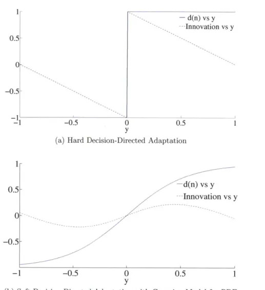
3-1 Plot of the "desired symbols" d(n) and innovation as a function of equalizer filter output y for BPSK system . . . . 45

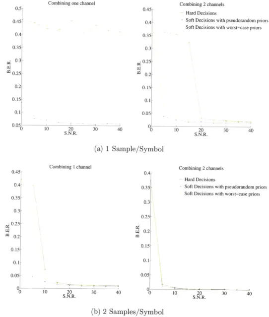
3-2 Results of Implementation of the Equalizer with Simulated Channel . 46 3-3 Equalizers Tested with SPACE08 Data . . . . 49

4-1 Simplified System Model for Analysis . . . . 52

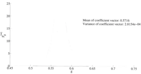
4-2 Distribution of the coefficient of a one-dimensional feedforward equal-izer equalizing a 2-tap channel, with A.W.G.N. . . . . 59

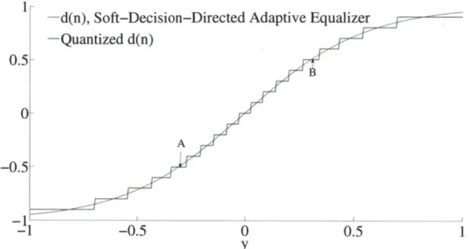
4-3 Plot of decision function and its quantized version for the soft-decision directed adaptive equalizer . . . . 64

4-4 1 tap equalizer for 2-tap channel under hard-decision directed adaptation 66 4-5 1-tap equalizer for 2-tap channel under soft-decision directed adaptation 68 4-6 Predicted Distribution of the Mean of the Coefficient Vector with 2 Feedforward Taps, Hard-Decision Directed Adaptation . . . . 69

4-7 Distribution of the Coefficient Vector from Simulation with 2 Feedfor-ward Taps, Hard-Decision Directed Adaptation . . . . 70

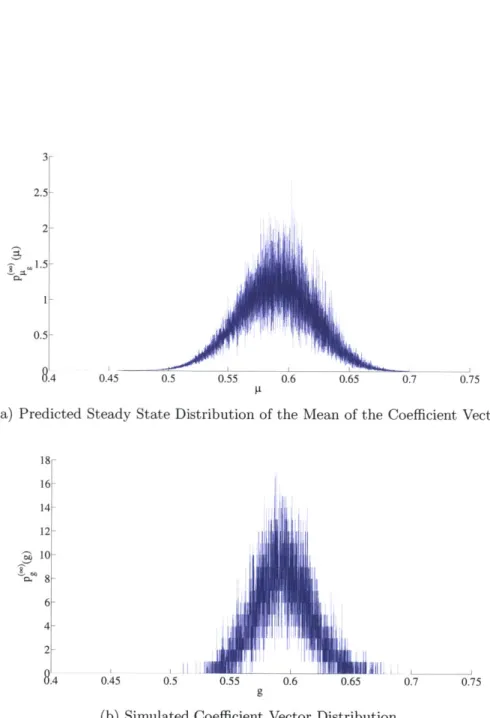
4-8 Predicted Distribution of the Mean of the Coefficient Vector with 2 Feedforward Taps, Soft-Decision Directed Adaptation . . . . 72

4-9 Distribution of the Coefficient Vector from Simulation with 2

Feedfor-ward Taps, Soft-Decision Directed Adaptation . . . . 73

4-10 Predicted Distribution of the Mean of the Coefficient Vector of DFE with 1 feedforward and 1 feedback tap, Hard-Decision Directed Adap-tation. Showing Failure Mode . . . . 77

4-11 Simulated Distribution of the Coefficient Vector of DFE with 1 feedfor-ward and 1 feedback tap, Hard-Decision Directed Adaptation. Showing Failure M ode . . . . 78

4-12 Predicted Distribution of the Mean of the Coefficient Vector of DFE with 1 feedforward and 1 feedback tap, Soft-Decision Directed Adap-tation. Showing Failure Mode . . . . 80

4-13 Simulated Distribution of the Coefficient Vector of DFE with 1 feed-forward and 1 feedback tap, Hard-Decision Directed Adaptation. Does not Fail Catastrophically . . . . 81

4-14 Plot of Probability of Catastrophic Failure in 7500 Symbols at Various SNRs... ... 82

4-15 Plot of Statistics of Equalizer Output Conditioned on s(n) = 1 . . . . 85

5-1 Turbo Equalizer- a High-Level Block Diagram . . . . 90

5-2 The Original Turbo Equalizer [11] . . . . 92

5-3 Turbo Equalizer- Transmitter . . . . 98

5-4 Turbo Equalizer- Receiver . . . . 98

5-5 Turbo Equalizer from [7]: Soft-Iterative DFE . . . . 100

5-6 Turbo Equalizer from [8]: Soft Information in Feedback Only . . . . . 101

6-1 KAM11 Mooring Positions Showing Locations of Transmitter and Re-ceiver . . . . 104

6-2 The Effect of Interelement Spacing on Performance, Training Mode Equalizer . . . . 105

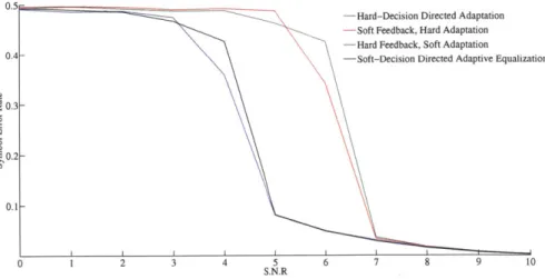
6-2 Plot of Mean Square Error of the Equalizer Output as a Function of Iteration at Various SNRs and for Different Turbo Schemes . . . . 114

6-3 Plot of Bit Error Rate of the Decoder Output as a Function of Iteration at Various SNRs for Various Soft Adaptation Based Turbo Schemes . 119 6-4 Results for Soft-Adaptive Turbo Equalizer, Soft-Adaptive Turbo

Equal-izer with Estimated Means and Soft-Iterative DFE at 24dB . . . . 123 6-5 Results for Soft-Adaptive Turbo Equalizer, Soft-Adaptive Turbo

Equal-izer with Estimated Means and Soft-Iterative DFE at 21dB . . . . 124 6-6 Results for Soft-Adaptive Turbo Equalizer, Soft-Adaptive Turbo

Equal-izer with Estimated Means and Soft-Iterative DFE at 18dB . . . . 125 6-7 Results for Soft-Adaptive Turbo Equalizer, Soft-Adaptive Turbo

Equal-izer with Estimated Means and Soft-Iterative DFE at 15dB . . . . 126 6-8 Results for Soft-Adaptive Turbo Equalizer, Soft-Adaptive Turbo

Equal-izer with Estimated Means and Soft-Iterative DFE at 12dB . . . . 127 6-9 Results for Soft-Adaptive Turbo Equalizer, Soft-Adaptive Turbo

Chapter 1

Introduction

Blue, green, grey, white, or black; smooth, ruffled, or mountainous; that ocean is not silent.

-H.P. Lovecroft Oceanography is a science born out of human desire to understand that important part of our world- the oceans. The oceans are where life on earth began, and they

hold secrets that continue to influence the course of human history.

In today's world, communication in any environment is an integral part of being able to understand and exploit it. The oceans are no exception. From submarines to undersea robotics, from fisheries to oil exploration- many problems in oceanography are dependent on the ability to perform underwater wireless communications over a range of distances.

This thesis explores one major aspect of wireless underwater communication sys-tems: adaptation algorithms for channel equalization. Adaptation algorithms are an important part of modern signal processing, and find applications in various fields, particularly in systems designed to handle time-variability. The primary objective of this thesis is to develop methods for the design and analysis of adaptation algo-rithms for practical communication systems, with the emphasis being laid on channel equalization for wireless underwater communication.

address with this work. We then present a bird's eye view of the traditional approaches to the design of systems for underwater communication. The chapter concludes with

an overview of the organization of the thesis.

1.1

The Challenges of Underwater

Communica-tion

The objective of underwater communication is to transmit data wirelessly over ranges of a few hundred meters to a few tens of kilometers. The range of electromagnetic waves underwater, however, is only a few meters. Therefore, RF communication is infeasible in the ocean environment. Optical communications are similarly only feasible up to a few hundred meters in clear water, and the ranges diminishes in turbid water.

The typical medium of communication underwater is acoustic waves, which propa-gate over the ranges of interest with reasonable signal levels. The underwater acoustic channel, however, is fraught with difficulties [53]. The channel impulse response is typically long and has multipath. As a result, it is subject to time varying Inter-Symbol Interference (ISI) and Doppler effects [38].

A sample channel impulse is shown in Figure 1-1. This was collected on Ju-lian Date 178, 2011 as part of the KAM11 Experiment off the coast of Kauai Island, Hawaii. This impulse response shows a long, time-varying channel. However, the spe-cific environmental conditions have a profound impact on the channel characteristics, making it hard to explicitly model such a channel.

1.1.1

The Need for Adaptive Equalization

Evidently, with such a long impulse response channel, we expect ISI to be a challenge at the receiver. We hence require an equalizer to be part of our receiver set up. An equalizer is a system of filters which is used to invert the response of a noisy channel in order to recover the symbols transmitted through the channel without blowing up

80 60 40 20 00 5 10 15 20 25 30 35 40 45 50 20 15 E 10 5 0 5 10 15 20 25 30 35 40 45 50 Time (s)

Figure 1-1: Channel delay spread- KAM11, Julian Date 178 at 1855

the noise (this is not a strict inversion, of course- it is implemented as an MMSE or Least Squares processor.

In a time-varying environment, the coefficients of the filter need to be varied with time. This is true also of a variety of environments including underwater communica-tion, mobile radio [40] and magnetic disk recording technology [9], for instance. The adaptation of these filters in practical environments and understanding the behaviour of the adaptation algorithms is the subject of this thesis. We begin with a study of history- by looking at the prior appoaches to underwater communication systems and how they tie in with the work presented here.

1.2

An Overview of Underwater Communication

Systems

A modern history of underwater communication systems probably begins with the 2nd World War. Advances in signal processing techniques have made it possible to

significantly improve the data rates, by implementing sophisticated signal processing algorithms at the receiver of the system.

We look at the various kinds of communication and signal processing algorithms and techniques that have been employed. This is necessarily a very brief and informal review. A much more complete review may be found in

[501.

We focus on the specific receiver structures that are relevant to the work presented here.

The major issue has been how we should design the system to combat the effects of time-varying multipath dispersion. Phase coherant techniques are required for reasonable data rates, but they are even further subject to these effects. So an array of sensors is used to allow for diversity to combat the multipath. The starting point, therefore is an array processor to mitigate the multipath dispersion. The resulting signal is treated as though it comes from a single ISI channel and is equalized. The optimal algorithms for such a structure are described in

[52].

The beamformer is typically followed by an adaptive equalizer. Due to its low com-plexity, reasonable convergence and tracking properties, the Recursive Least Squares (RLS) algorithm is known to be a good choice of adaptation algorithm [23]. The adaptation algorithm is usually trained with some known data, and then used in decision directed mode.

We distinguish between 2 kinds of equalization - channel estimation based equal-ization and the so called direct-form equalequal-ization. In channel estimation based adap-tive equalization, the channel impulse response is explicitly estimated. Using the channel impulse response, an optimal equalizer can be formulated based on any one of a number of criteria [20].

On the other hand, in direct-form equalization, the equalizer coefficients are di-rectly computed from the output of the channel. The emphasis of this thesis is on this form of equalization. This form of filter is preferred due to ease of implementation and low complexity. However, the algorithms for adaptation and methods of analysis that we will present can be used for channel estimation type approaches as well, with some modifications.

Fre-:1 1 ! 1: ~i 111 IClia % 1 1:1cl II I nel earnorme Adaptive D c dn

Data Coding Modulation Channel Beamforme Decoding Received Data

JNoise

(a) Basic Block Diagram

D Coding Modulation Channel Beamioer J Apiv te R edoding

Data IC ~ Equalizer oDReceived Data

+ Infonnation

Noise

(b) Turbo-Equalizer Block Diagram

Figure 1-2: Block Diagrams of Communication System

quency Division Multiplexing (OFDM) [51]. While this has a lower cost of complexity of equalization, OFDM receivers are subject to severe Doppler effects. We will not focus on this technology in this thesis, but they have been the subject of research in the underwater acoustics community in recent times. (See, for instance, [29] and [25]).

In general, forward error correction coding is applied to the data before transmis-sion. This adds redundancy and enables us to further improve the performance of the communication link. The standard block diagram in Figure 1-2a of the commu-nication system, which shows how these components fit together.

The advances in the subject of near capacity achieving codes have led to the development of sophisticated turbo codes [19]. It was realized that a similar concept could be applied to equalization, where the equalizer was treated as a kind of decoder. This led to the principle of turbo equalization [27], depicted in Figure 1-2b. Here, the equalizer and decoder iterate and exchange the so-called soft information. This information is used by the other block in the next iteration. For a more detailed exposition of turbo equalization, see [26]. Turbo equalization has been applied to the underwater communication in [48], [8], among others. We will show that the algorithm we derive has application as an adaptive turbo equalizer, and will very naturally fit into the turbo framework.

We conclude this section with a note on Faster-than-Nyquist (FTN) signaling, which was originally introduced in [32]. This technique has recently found application to the channels of our interest [13]. It can increase the data rate without increasing

the bandwidth. However, this is at the expense of lengthening the channel impulse response, increasing the amount of ISI in the channel. Therefore, we require a good adaptive equalizer to take advantage of this method. This is another use of the improved equalizer that we present here.

1.3

Thesis Organization

This thesis is organized as follows: in Chapter 2, we provide a detailed introduction to the system layout and the RLS Algorithm. We formally describe the problem that we will attempt to solve in the thesis.

Chapter 3 contains the derivation of the soft-decision directed RLS adaptation algorithm from the EM Algorithm. In this chapter, we also build connections to blind equalization techniques which are prevalent in literature and show how the algorithm bridges the gap between the maximum likelihood based EM Algorithm and these practical approaches.

In Chapter 4, we analyze the performance of adaptive equalizers under decision directed adaptation. We also analyze the performance of the algorithm that we derive and show why we expect this to do better. This chapter also explains what insights the analysis holds for further development of the algorithm.

Chapter 5 considers a practical implementation of a turbo-equalizer system based on the soft-decision directed RLS algorithm. We demonstrate how this compares to existing turbo equalization approaches, and the choices of what kinds of codes to use in the turbo equalizer.

We then demonstrate the practical applicability of the system in Chapter 6 by testing it with actual data from the KAM11 Acoustic Experiments. The experimen-tal setup and transmitted signals are presented in detail, and a comparison of the

algorithm against the existing algorithms in the field is carried out.

Finally, Chapter 7 summarizes the results presented in the thesis, and suggests possible directions for future work.

Chapter 2

Preliminaries

2.1

Notation

Table 2.1 contains the notations that are used in the rest of the thesis without redef-inition.

2.2

System Model

The block diagram of the system of interest is shown in Figure 2-1. This is the diagram of the channel and an adaptive decision feedback equalizer. In this section we describe how the different blocks operate and the mathematical models that we use for the system. The thin solid lines represent the flow of data in the equalizer and the dotted lines represent the flow of information to and from the adaptation algorithm used to adapt the coefficients of the filter. We will modify the system model as required in later chapters. A few points are worth mentioning at this stage. This diagram is incomplete in the sense that it does not include a turbo loop (a feedback loop from the decoder to the equalizer). This is done for clarity's sake. We will describe the turbo structure more in Chapter 5, and will introduce the feedback loop at that juncture.

Also with reference to Figure 1-2a, we note that we have not included a beam-former or array processor explicitly in Figure 2-1. This is because practically, we

Symbol Type

x (non-boldface math symbol) u (boldface, lowercase symbol) A (boldface, uppercase symbol)

IN

p(

-)

IP'(-) * T H

Scalar constant or variable

Column vector (size inferred from context) Matrix

N x N identity matrix (without subscript, size inferred from context)

probability distribution function, semi-colon indicates parametrization by a deter-ministic, but unknown quantity following the semicolon.

probability distribution function, pipe op-erator I indicates conditioning.

P.D.F. of Multivariate Normal Distribu-tion with mean y and covariance matrix Indicates distribution of random variable, eg., x ~ .N(O, 1) means random variable x is distributed as a standard normal vari-able.

Expectation of the quantity in the square brackets with respect to the p.d.f. specified in the subscript

Probability of the event in brackets Complex Conjugate

Matrix Transpose Matrix Hermitian

Table 2.1: Notations used in the thesis

Adaptation

Channel +

s (n) h, (-)

.(n)

Figure 2-1: Block Diagram of Direct-Form Adaptation Equalizer Meaning

can implement the multichannel processor by stacking up the inputs from different channels into an equivalent feedforward input vector. The beamforming then happens implicitly within the equalizer.

2.2.1

The Channel

At the transmitter end, we define s(n) as the symbol transmitted at time n. The symbol passes through a channel, which introduces ISI. The channel also introduces random noise, represented by v(n) at time n. Thus, corresponding to the symbol transmitted at time n, we have a received signal at the output of the channel, which we denote by x(n). M is the length of the channel response. This means that the output of the channel at time n depends on symbols s(n), s(n - 1), . . ., s(n - M - 1). If h (-) is the channel response at time n, then we write

z(n) = hn(s(n), s(n - 1,...,s(n - M - 1)) + v(n) (2.1)

Note that we assume that the channel response is causal. We may do this with no loss of generality, because all we would need to do is introduce a suitable delay into the receiver if it is not. We will assume a linear (but time-varying) channel, so we can write the channel filter coefficients hk(n), k = 0, 1, ... , M - 1 as channel coefficients at time n. The channel output is then a convolution, given by

M-1

x(n) = h*(n)s(n - k) + v(n) (2.2)

k=O

We define the channel vector, h(n), as:

h(n) = ho(n) ... hM-1 (n)] (23)

2.2.2

The Equalizer Filters

The receiver end is a Decision Feedback Filter (DFE), which has 2 filters: a feed-forward filter gf of length Nf and a feedback filter g of length Nb. The purpose

of the feedforward filter is to invert a portion of the channel impulse response while ensuring that it does not blow up the noise that is present in the received signal. The feedback filter cancels out residual ISI by subtracting out past symbols (or decisions) from the output of the feedforward section. Intuitively, the feedforward filter inverts the channel, and the feedback filter subtracts out the remaining ISI. We define the total equalizer dimension as N - Nf + Nb.

The input to the feedforward filter at any time n is the past Nf symbols at the output of the channel, which we denote by x(n)

x(n) = x(n) x(n - 1) -.-. x(n - Nf - 1)] (2.4) Similarly, we denote by d(n) the decision made by the system at time n. This is an estimate, in some sense, of the transmitted symbol. We shall discuss what we mean by estimate in this context more in detail later. The input to the feedback filter at time n can thus be denoted by z(n), where

z(n) = [z(n - 1) z(n - 2) - z(n - Nb) (2.5)

As these filters are adaptively varied, we specify the time at which we are looking at the filter coefficients. We denote by gf(n In - 1) and gb(n n - 1) the respective

feedforward and feedback filters used to filter the data at time n, computed given all the data up to (and including) time n - 1. Then, the output of the equalizer at time n, which is denoted by y(n) is given by

y(n) = gfH(tn - 1)x(n) - gbH(nln - 1)z(n) (2.6)

We can significantly simplify notation by defining a consolidated "overall" filter coefficient vector, denoted simply as g(nln - 1) at time n, by

g(ngn - 1) = (2.7)

I)-Correspondingly, define the overall input vector to the equalizer u(n) as

u(n) =

]

(2.8)

z(n)-Then Equation 2.6 can be written more simply as

y(n) = gH(nn - )u(n) (2.9)

The form of the equalizer operation represented by Equations 2.7-2.9 allows for a great flexibility in choosing the form of equalizer. For instance, we need not treat linear feedforward equalizers any differently in the mathematical framework, as long as we make the right assumptions on the input vector.

2.2.3

The Channel Transfer Matrix

We also define a channel transfer matrix H(n) that relates the transmitted symbols to the overall input vector u(n). We note that x(n) depends on symbols s(n), s(n

1),. . ., s(n M 1), and x(n Nf 1) depends on symbols s(n Nf 1,..., s(n

-Nf - 1- M - 1). Also, assuming no error propagation, the feedback filter has symbols

s(n - 1), ... , s (n - Nb). Thus, the input depends on s(n), s(n - 1), ... , s(n - P), where P = max(Nf + M - 2, Nb). The P x N channel transfer matrix (with no error propagation in the feedback filter)

ho(n) 0 0 0

hi(n) ho(n - 1) 0 INb

. ho(n - (Nf - 1)) H(n) hM1(n) hM-2(n - 1) (2.10) 0 hm-1(n - 1) 0 0 . hM-1(n - (Nf - 1)) 0 0 0 - PxN

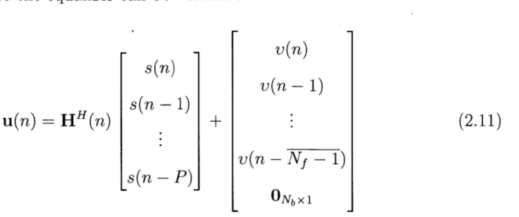
and the input to the equalizer can be written as v(n) s(n) v(n -1) s(n - 1) u(n) = H(n) (2.11) v(n - Nf - 1) -s(n P)

Note that if we assumed there was error propagation, i.e., the symbols in the

feedback filter were not perfect, there would be a complex, non-linear relationship

between the input to the feedback filter and the transmitted symbols, and the simple

matrix relations of Equations 2.10 and 2.11 would not be sufficient to describe it.

2.2.4

Outputs and Decisions

y(n) is mapped by the decision device into an estimate of the symbol used in the adaptation and feedback filters, which we denote as d(n). It is important to note that the estimate used for adaptation may not be the same as the one used for the feedback filter in general. By default, we will assume this, but it is not important to the derivations presented, as will become clear. In cases where it is important, it will explicitly be stated what assumptions are being made. Finally, y(n) is also mapped into an output decision based on what we need at the decoder or the next component of the system (or hard decisions if this is the final stage).

Table 2.2 summarizes the most important of the quantities which we have defined in this section. We now move to describing the purpose of the "Adaptation" block

and the algorithms used for it. This will lead us to describing the problem of interest.

2.3

The Adaptation Algorithm

Since the channel is time-variant, the equalizer coefficients must be varied with time.

Symbol Quantity Represented

Symbol transmitted at time n Channel Impulse Response length Feedforward filter length

Feedback filter length

Total filter length, Nf + Nb

Number of symbols on which equalizer input de-pends, given by P = max(Nf + M - 2, Nb)

Overall input to the equalizer

fil-ters corresponding to s(n), given by

[x(n)...(n-Nf- 1),z(n- 1)...z(n-Nb)] T

Overall coefficient vector to filter input at time n, computed given data up to (and including) time n - 1

Output of equalizer corresponding to s(n)

Estimate of s(n) used in feedback filter and adap-tation

Any general decision rule that is used to map y(n) into decisions used in the feedback filter and/or in adaptation, such that d(n) = T(y(n))

Table 2.2: Summary of Important Symbols Defined for the System s(n) M Nf Nb N P u(n) g(nln - 1) y(n) d(n) TW)

is what we will consider for the rest of the thesis.

Mathematically stated, the purpose of the adaptation algorithm is to adaptively choose a set of coefficients g(nn - 1) to filter the input signal u(n), based on a knowledge of the inputs u(1), u(2), . .. , u(n - 1), and a set of desired symbols

d(1), d(2),... d(n - 1). The desired symbols are the desired outputs of the adaptive

filter. In our case, therefore, they should theoritically be the transmitted symbols

s(1), s(2), ... , s(n - 1). We may, however, only have probabilistic information about

s(n). Traditionally, the symbols are assumed known at the receiver, and this is the context in which algorithms like RLS are usually implemented.

While a detailed account of the recursive algorithms used in many applications (including equalization) may be found in [20], [31] and [42], among many others , we consider one very important adaptation algorithm, called the Recursive Least Squares

(RLS) Algorithm.

2.3.1

Recursive Least Squares

One common approach to implementing equalizers is using the coefficients g(nIn - 1) that are optimal under the Least Squares criterion. This is because it is the Maximum-Likelihood estimator under a known transmitted signal and a Gaussian observation noise assumption for time-invariant channels. Possibly more importantly, it works very well in practice, and an efficient recursive solution exists [20].

The least squares approach is to estimate a system g(n + 1 In), given observations

u(1), . . . , u(n) and desired signals s(1), .. ., s(n) so that we minimize a cost criterion

given by:

n

Jn(g) = An ms(m) - gHU(m)1 2 (2.12)

M=1

where A < 1 is an exponential weighting factor, designed to give us tracking ability. More specifically, it limits the "averaging window" and thus allows the estimator to remain responsive to additional observations as they are received. A, therefore accounts for the time-variance of the system. A = 1 would imply infinite memory, and would be optimal for a time-invariant system. Any A < 1 lets us track a dynamic

system.

It may be shown that the coefficient vector that minimizes this is given by

g(n + 1|n) =Ru'(n) A n-mu(m)s*(n) (2.13)

where Ru(n) is the sample autocovariance matrix of the process, given by n

RS(n) = An-mu(m)uH(m) (2.14)

The RLS algorithm is a computationally efficient way to obtain the solution of

(2.13). At each time n the algorithm computes the new coefficient vector g(n) from

the previous coefficient vector as

g(n + 1|n) = g(nrn - 1) + k(n)(s(n) - gH(r n - 1)u(n))* (2.15)

k(n) is the Kalman Gain vector, defined by

k(n) = Rul(n)u(n) (2.16)

We define the term e(n) = s(n) - gH(n n - 1)u(n) = s(n) - y(n) as the innovation at time n.

2.3.2

Hard-Decision Directed Adaptation

It is evident from Equations 2.13 and 2.15 that the RLS adaptation procedure depends

on the transmitted symbols s(n). Most conventional adaptation algorithnms have this requirement. In communication systems, though, we cannot have access to this information.

Thus the usual procedure in such cases is to first transmit a sequence of symbols which is known at the receiver end. Such a sequence is called the training or pilot sequence. This is used to train the equalizer. Following this, the equalizer is switched

R(y) < 0 R(y) > 0

a(y) > 0

!a(y) > 0

R(y)

R(y) < 0 R(y) > 0

a(y) < 0 a(y) < 0

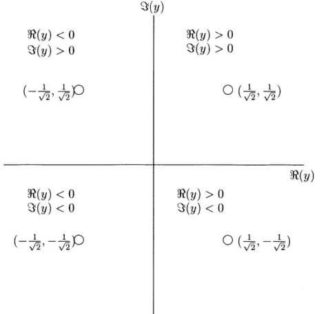
Figure 2-2: Q.P.S.K. Constellation and Output Decision Regions

into the so-called hard-decision directed mode.

In hard-decision directed mode, the equalizer maps the filter output y(n) to the nearest constellation point. For example, Figure 2-2 shows how this is done with a Q.P.S.K. constellation and the corresponding decision regions on y(n). This decision, which is denoted dh(n), is used in adaptation instead of the true transmitted symbol s(n). That is to say, Equation 2.15 now becomes

g(n + 1 |n) = g(n n - 1) + k(n)(4h(y(n)) - g - *

= g(nn -- 1) + k(n)(dh(n) -gH(m 1)u(n))* (2.17)

where Wh(-) represents the operation of the hard mapper. This is termed hard-decision directed adaptation, as the hard-decisions made to be used in the adaptation process are hard decisions on the symbols. However, this procedure is suboptimal. We will intuitively see this in the next section, which will lead us to the statement of

the problem we seek to address in this thesis.

2.3.3

Soft Information in Adaptation

Consider, with reference to the Q.P.S.K. constellation of Figure 2-2, the points y(n)

-(0.1, 0.1) and y(n) = (0.7, 0.7). Both of these in the hard-decision directed scheme would be mapped to the constellation point (1/.,1 /,). In fact, the innovation is larger in the first case and the algorithm makes a bigger correction to the coefficients.

However, there is larger likelihood that y(n) = (0.1, 0.1) is a result of an error made in the filter output due to noise than the second case of (0.7, 0.7). This would mean that we would be adapting to the wrong symbol, and as we make a bigger correction, we would be introducing a larger error into the coefficients computed for the next time instant. These errors are not correctible in the future, as we assume that the algorithm is purely recursive (i.e., we do not "go back in time" and correct errors). So in hard decision directed adaptation, we hope to make sufficiently small numbers of errors so that the coefficients are still reasonably correct.

It is evident, though, that we are losing information, so the question becomes whether there is a computationally efficient way of using that information in adapta-tion as well. We define as soft informaadapta-tion any probabilistic informaadapta-tion about the transmitted symbols that we can take advantage of in the adaptation process. The information about how likely it is that a particular filter output is due to an error is considered soft information. We will also interpret the definition to include priors or other information on the symbols that we may have available as a result of other components of the system.

2.4

The Problem Statement

We state the problems of interest in this thesis as follows:

e What adaptation process can take advantage of the soft information available to it? This question can be posed in 2 cases

- When the equalizer is being run with no prior information about the sym-bols, i.e., the soft information consists only of quantities that can be com-puted from the filter output.

- When some prior information is available to the equalizer about the trans-mitted symbols

" How much performance do we lose when we adapt in hard-decision directed mode, as opposed to adapting with known symbols? And how much can we improve this by a different algorithm?

" How do we design a practical turbo-type system from this algorithm using the priors that are always available in such a system?

In the following chapters, we address each of these issues. First we derive an adaptation algorithm that can utilize soft information, and show it to be optimal in an Expectation Maximization sense. We then analyse the performance of equalizers under hard-decision directed adaptation and the algorithm that we derive and develop understanding into their operation. Finally, we design and demostrate practical sys-tems using this algorithm. In particular we design a turbo equalizer, which we have not introduced in this chapter. We will do so in Chapter 5.

Note that we thus focus on the effect of the adaptation algorithm on the perfor-mance of practical systems in which adaptation is required. While we attempt to keep the discussions as general as possible, we will specifically refer to the equaliza-tion setup during the derivaequaliza-tions. We also do not focus on the effect of errors in other components of the system (specifically, the feedback filter. Error propagation in the feedback filter has been an emphasis of prior research- see, for instance,

[14],

[44] and [46]).

Chapter 3

The Recursive Expected Least

Squares Algorithm

We introduced the problem of reliable adaptation when we do not know the transmit-ted symbols in section 2.4. In this chapter, we derive a recursive procedure, relatransmit-ted to the RLS algorithm, which is specifically designed to perform adaptation under this constraint. This procedure will be designed to take advantage of whatever infor-mation is available at the receiver output, and is thus inherently more reliable than hard-decision directed equalization. The derivation will take the following steps

[59]:

first we look at how the problem of adaptation without knowledge of the transmit-ted signals can be viewed as an Expectation-Maximization type problem. This, along with analogies to the least-squares approach, will let us define a suitable cost criterion that does not depend directly on the tranmitted signals. Then we can approximate the solution to this cost criterion by a purely recursive algorithm, which will let us im-plement this algorithm practically with a small price to pay in terms of computational efficiency over conventional RLS.

3.1

The First Step: the Expectation-Maximization

Algorithm

The Expectation Maximization (EM) Algorithm [10] is a powerful algorithm for per-forming Maximum-Likelihood (ML) Estimation of the parameters of a system when all the data about the system is not available. We will start from an ML frame-work, as this is easiest in the context of the EM algorithm, and relate this to a more computationally efficient least squares framework later.

What, however, does parameter estimation have to do with this system? At any time n, we could treat g(n + 1 n) as a parameter of our system which maps u(n) into y(n), an estimate of s(n). The key insight here is that we can treat s(n) as a random variable. This is a common approach in Bayesian estimation [28]. Thus, when we don't have access to s(n), we have an incomplete set of observations, and wish to perform parameter estimation! This leads us to the intuition that we could somehow set up this problem in an EM framework.

We start by assuming that g(n

+

1|n) can be treated as a time-varying, determin-istic (but unknown) parameter of a system characterized by a full set of observations

y(n) = [y(n) y(n - 1) - -- y(1)1 and s(n) = [s(n) s(n - 1) ... s(1)1. We note

at this stage that the actual set of observations is u(n), u(n - 1),... , _{u(1) and s(n),}

and using y(n) in the place of the u(n) vectors may lead to a loss of information, as the mapping between u(n) and y(n) is not necessarily one-to-one. However, the structure of the direct adaptation equalizer is such that u(n) depends linearly on the channel coefficients, as opposed to the equalizer coefficients. The relationship be-tween the equalizer coefficients and the channel coefficients is non-linear, even when the equalizer is optimal [38].

Hence, characterizing u(n) in terms of the parameter of interest g(n+1|n) is hard, making u(n) infeasible to work with. But why is working with y(n) easier? This is an idea that falls out of our understanding of the EM procedure. With a knowledge of how the observed data depends on the parameter which we are trying to estimate, and a guess of the parameter, EM generates guesses about the data which is hidden.

The output of the equalizer itself is related to the transmitted signal s(n) in a probabilistic manner, where the probabilities depend on the "parameter"- the equal-izer coefficients. Using the current estimate of the parameter, g(nIn - 1), we can generate the "observable data", y(n), and use that in some probabilistic sense to generate estimates of the "hidden data", s(n). This can then be used to compute a new estimate for the parameter, g(n

+

1|n).

To recap, therefore, the reason for using y(n) rather than the true observed data u(n) is that we have a simple relationship between y(n) and the parameter that we are trying to estimate. A similar relationship is not easy to find between u(n) and the equalizer coefficients. Thus, we allow the many-to-one transformation which depends on the coefficient vector, and use its output as the observed data. Note, however, that we do still have access to the equalizer input.

The procedure that we discussed sounds almost exactly like conventional EM, except that now the data and the parameters are all time-varying and we want to keep complexity low. We thus start the derivation by following a procedure similar to the derivation of the EM algorithm in [24]. The maximum likelihood estimate of the parameter g(n

+

1 n) at time n, given the complete data (y(n) and s(n)) up to time n, would be given by

gML, complete(n + 1 n) arg max [log p(s(n), y(n); g) g

- arg max In(g) (3.1)

g

When we do not observe any of the symbols s(n), a reasonable objective is to maximize the log-likelihood of the data we have, which is simply y(n). So we want to determine the maximum likelihood estimate of the parameters given the (incomplete) data, i.e.,

gML, incomplete(n + 1 n) = arg max [log p(y(n); g)

g

arg max In(g) (3.2)

While directly computing this is hard, we observe that:

I,(g)

= log p(y (n); g)

- log 1 p(y(n), s(n); g)

s(n)

- loge p(y(n), s(n); g)q(s(n) y(n))

q (s(n)| y(n))

s(n)

> 1 q~ (n Iy ()) ogp (y (n), s (n); g) S2 n q n))yIn))log (s

En (q(s (n)|Iy (n)), g) (3.3)

where q(s(n)|y(n)) is any valid probability distribution function , which we use for averaging. The function En(q(s(n) y(n)), g) is called the auxilliary function for the data up to time n. This is a standard definition in the derivation of the EM Algorithm (see, specifically, [24]).

The inequality in Equation 3.3 follows directly from the measure-theoritic form of Jensen's Inequality for concave functions, and it shows that the auxilliary function lower bounds the function we want to maximize. Now, like we do with the iterative EM algorithm, we can define a 2 stage process everytime we receive new data, as

follows:

Q(s(n)|y(n)) = arg max En(q(s(n) y(n)), g(nIn - 1)) E-Step (3.4)

q(.I-)

g(n + 1|n) = arg max L4( (s(n) y(n), g) M-Step (3.5)

g

At this stage we note the difference between the conventional EM algorithm and the procedure defined in Equations 3.4 and 3.5, which we call the Recursive EM procedure. In conventional EM, we have a single dataset. We repeatedly perform the E-step and M-step on the same dataset and it can be shown that the procedure converges to a local maximum of the auxilliary function [58].

However, the procedure we are defining as recursive EM operates only once on

new data received at time n

+

1. That is, at each time n, we run the E-step and M-step once each, and call that our new estimate. Put another way, our time index is also our iteration index. The conventional EM algorithm, on the other hand only has an iteration index.

Note that there is nothing to stop us from performing multiple iterations at each time until convergence occurs. We choose not to do so for computational reasons, but we do not guarantee that the algorithm converges at each time.

Back to the derivation. To solve Equation 3.4, substitute

q(s(n) y(n)) = p(s(n) y(n); g(nln - 1)) (3.6)

into Equation 3.3 . Then,

ECn(p(s(n)ly (n)), g(n In - 1))

p(y (n), s(n); g(n n - 1))

Z

p(s(n) y(n); g(nn - 1)) log p(s(n) y(n); g(nln -1))

s(n) p(s(n)|y(n); g(nln - 1))

= p(s(n)|y(n); g(nn - 1)) -log p(y(n); g(nln - 1))

s(n)

log p(y(n); g(nln - 1)) -, p(s(n) y(n); g(nn - 1))

s(n)

=log p(y(n); g(nln - 1))

ln(g(nln - 1)) (3.7)

But Equation 3.3 shows that for any (q(..), g) pair, En(q(s(n) y(n)), g) < In(g). The probability distribution used in Equation 3.7 causes equality to hold, implying that for g = g(nln - 1), the probability distribution that maximizes the auxilliary function and hence solves Equation 3.4 is given by:

q(s(n)|y(n)) = argmaxEn(q(s(n) y(n)), g(nln - 1))

q(.I)

Finally, Equation 3.5 can be replaced by a maximization of an expectation with respect to q(.|) of the complete log-likelihood instead of C(-,-) for any q(-), as shown below,

arg max E(q(s(n)|y(n)), g)

g

arg max q(s(n)y(n)) log s(n);g)

g s(n) q(s(n)|y(n))

arg max 13 q(s(n) y(n)) log p(y(n), s(n); g)

g s(n)

- q(s(n)Iy(n)) log q(s(n) y(n))

s(n)

= arg max 1 q(s(n) y(n)) log p(y(n), s(n); g)

g s(n)

= arg max Eq(s(n)|y(n)) [log p(y(n), s(n); g)] (3.9)

g

Combining Equations 3.8 and 3.9, we have a single equation that captures the results of the derivation so far:

g(n + 1| n) = arg max Ep(s(n)ly(n);g(njn- 1)) [log p(y(n), s(n); g)] (3.10)

g

To summarize, at each time n when a new input vector u(n) is received, we map it into a new observed data point y(n) for the recursive EM algorithm using the current estimate of the parameter. Then, using the probability density function of the hidden data s(n) conditioned on y(n) and parametrized by the current coefficient vector, we find the expected log-likelihood of the complete data. Then, we perform one

maximization of this over the parameter space to form the new estimate g(n + 1|n), and then stop and wait for more data. Observe that this in itself is a partly recursive solution, because we update the estimate only when we get new data.

However, while we have defined what to maximize (and why) we have said nothing about how. Maximizing the expected log-likelihood in Equation 3.10 could be quite computationally intensive. Thus, we first change the log-likelihood based criterion

above to a least-squares type criterion. We can then derive a solution for it, which can be simplified to be recursive and causal.

3.2

The Expected Least Squares Cost Criterion

One possible way to think about the Least Squares Cost Criterion defined by Equation 2.12 is that it is Maximum Likelihood Estimation for Gaussian variables [28,31]. Put another way, the least squares sum is a sufficient statistic for parameter estimation with Gaussian variables in a fully observed system.

To see this, consider a time-invariant fully observed system (i.e. we observe both u(n) and s(n). Assume y(n) = s(n) + y(n), where 77(n) represents all the residual interference at the output of the equalizer, and q(n) is Gaussian with mean 0 and variance or. Then,

nsm - gH U(n12

gML,Gaussian= arg max exp

(-

s(m) 2um2

-9 (m=1

n

= arg min

Is(m)

- gIu(m)12]

9 m=1

= gLeast Squares (3.11)

Now suppose that s(n) does not depend on g(n

+

1|n) (which is reasonable), and that y(n) is Gaussian given s(n) (which, as we will see later is not a perfect assumption). Then it is evident that we can write Equation 3.10 as

g(n + 1|n) = arg max [Ep(s(n)1y(n);g(nIn- ₁))[log p(y(n), s (n); g)]

n

= arg min Ep(s(n)ly(n);g(nln-1)) s(m)

-

gu )12 (3.12)

9 _n=1

We now choose this as our cost criterion, i.e., rather than using the expected log-likelihood, we shall henceforth use the expected least squares criterion. This is our cost criterion whether or not the distributions are Gaussians. We merely use

Gaussianity to justify the least-squares approximation.

However, we make one modification to the cost criterion in Equation 3.12. As is usually done with least-squares for time-variant systems (see [20]) we introduce an exponential weighting factor A < 1 to allow tracking of the time-variant features of the system (section 2.3.1). So the cost criterion we finally work with, which we term the Expected Least Squares cost criterion, is defined by

Jn(g) = Ep(s(n)|y(n);g(nn1)) A" ,|s(m) - gHu(m)12 _m=1

We assume henceforth that the expectation is with respect to the distribution p(s(n) y(n); g(nn - 1)) unless otherwise mentioned, and drop the subscript.

3.2.1

Solving the Expected Least Squares Criterion

A closed form solution exists for the minimum of in(g). To start with,

Jn(g) = E An-s(m) - gHU(M)2 _m=1 = A -m_IE[Is(m) - gHu(m)121 m=1 n

= A n-mE[(s(m) - gHU(m))(*(m) -u(m)g)] _(3.14) rn-i

To determine the minimum point of this function, one method we can use is to treat g and its Hermitian, gH, as 2 different variables. Then, we can write Jn(g)

in(g, gH), and it can be shown that the minimum of this function with respect to g

occurs at the point such that its partial differential with respect to gH is 0 (details of this may be found in Appendix B of [20]). As u(m) is known for all m, we can simplify Equation 3.14 as follows:

8JA(H gH m i n-mE[u(m)(s*(m) - uH(m)g)] = 0 (3.15)

Now, we pretended that the data for the recursive EM procedure was y(n) rather than u(n) vectors, in order to be able to parametrize easily. However, we know the value of u(m) for all m- it is just the input to the equalizer. So there's no need to take an expectation on this- we're essentially conditioning on it here- so that the above becomes: n

S

A n-,(u(m)d*(mln) - u(m)uH(m)g) = 0 (3.16) where d(mnl) = Ep(s(n)ly(n);g(nn-1))[s(m)1 = s(m)p(s(n)|y(n); g(nn - 1)) s(n) = s(m) p(s(m), s(n)\{s(m)}|y(n); g(nln - 1) s(m) s(n)\{s(m)} = s(m)p(s(m)|y(n);g(nrn - 1)) s(m) -E[s(m)|y(n); g(nln - 1)] (3.17)

Rearranging Equation 3.16, we can write the closed form minimization to the ELS cost function as

g(n + 1|n)= RU(n) An-mu(m)d*(mn) (3.18)

where Ru(n) is defined in Equation 2.14.

3.3

A Purely Recursive Approximation

The solution which is defined in Equation 3.18 cannot directly be written in a recursive form. This is because at each time n we need to compute the expectation of each of the past symbols given all the data upto and including n. When we get new data, therefore, we need to go back and update all the past "desired" values, d(mln), m < n. However, if we now constrain the system to be causal, so that we do not go back

and update the expectations of the past symbols, we have g(n

+

1|n) given by:

g(n + 1|In) = R-1(n) A- m_{u(m)E[s(m) y(m); g(mlm - 1)]*}

rn-i

= R- 1_{(n) A -mu(m)d*(m) (3.19)}

where d(m) is now defined by

d(m) = E[s(m) y(m); g(mlm - 1)] (3.20)

This is a sub-optimal approximation to Equation 3.18. However, the sequence d(n) is causal. From a comparison of Equation 3.19 with Equations 2.13 and 2.15, it is then clear we can define a recursive solution like Equation 2.15 by replacing s(n) with d(n), and treating this as the new "desired sequence" of symbols. Hence, a recursive algorithm, for which we don't need to go back and update or perform matrix inversions is obtained, which we call the Recursive Expected Least Squares (RELS) Algorithm.

g(n + 1|n) = g(nn - 1) + k(n)(d(n) - gH( H i - 1)u(m))* (3.21)

From a system point of view, this amounts to changing the decision device T(-) of Figure 2-1 from a hard slicer to d(n). But notice that d(n) is simply the Bayes Least Squares estimate of s(n) given the data y(n), parametrized by the current estimate of the underlying parameter of the distribution relating the symbol to the data g(njn - 1). This is an intuitively pleasing result, because it means replacing the unknown symbol with the statistically optimum estimate of s(n) given the data and the current parameter estimate.

While the decision device has this satisfying result, we emphasize that it is not the output of the decision device itself that is of primary interest. We are concerned rather with what effect this has on the adaptation process. Our derivation has given us one possible way to perform this adaptation in the absence of s(n).

3.4

Modelling the Probability Density Function

At the very outset, we note that computation of d(n) may not be trivial. In the most general case, we would have to implement some form of MAP estimator to compute the value of d(n) from the data, which itself might be computationally intensive. So let us look at the computation in more detail and attempt to simplify the computation. Define a dummy variable s'(n) which is distributed as s(n).

d(n) = E[s(n) y(n); g(nn - 1)] = s(n)p(s(n) y(n); g(nn - 1)) s(n) s (n) Z s'(n) P (y (n) Is'(n); g (njIn - 1)) p(s'(n)) YZ(n) (n) p(y(n) s(n); g(n n - 1))p(s(n)) Zs(n) p(y(n) s(n); g(n I - 1))p(s(n))

We assumed in Equation 3.22 that the symbol probabilities don't depend on the

system parameters. Further, we assumed in section 2.2 that the system is causal, so the data at times m < n is independent of s(n). Then,

p(y(n)|s(n); g(nn - 1)) = p(y(n),y(n - 1)|s(n); g(n~n - 1)) = p(y(n) y(n - 1), s(n); g(n~n - 1)) x

x p(y(n - 1) s(n); g(nIn - 1))

= p(y(n) y(n - 1), s(n); g(nIn - 1))p(y(n - 1); g(nn - 1))

(3.23)

Substituting equation 3.23 in equation 3.22, and observing that the second term does not depend on s(n), we have

Zs(n) s(n)p(y(n) y(n - 1), s(n); g(rI - 1))p(s(n)) (3.24)

d(n) =(.4

Es(n) p(y(n)ly(n - 1), s(n); g(n n - 1))p(s(n))