-1
The Directed Steiner Network Problem is
Tractable for a Constant Number of Terminals
by
Jon Feldman
Submitted to the Department of Electrical Engineering and Computer
Science
in partial fulfillment of the requirements for the degree of
Master of Science
at the
MASSACHUSETTS INSTITUTE OF TECHNOLOGY
June 2000
@
Massachusetts Institute of Technology 2000. All rights reserved.
A uthor ... . .-. ... .. ...
Dep rtment of Electrical Engineering and Computer Science
May 19, 2000
....Certified by
David R. Karger
Associate Professor
Thesis Supervisor
/Accepted by...
Arthur C. Smith
Chairman, Department Committee on Graduate Students
MASSACHUSETTS INSTITUTE OF TECHNOLOGY
The Directed Steiner Network Problem is Tractable for a
Constant Number of Terminals
by
Jon Feldman
Submitted to the Department of Electrical Engineering and Computer Science on May 19, 2000, in partial fulfillment of the
requirements for the degree of Master of Science
Abstract
We consider the DIRECTED STEINER NETWORK problem, or the POINT-TO-POINT
CONNECTION problem. Given a directed graph G and p pairs {(si, ti), .. ., (s,, tp)} of
nodes in the graph, one has to find the smallest subgraph H of G that contains paths from si to tj for all i. The problem is NP-hard for general p, since the DIRECTED STEINER TREE problem is a special case. Until now, the complexity was unknown for constant p > 3. We prove that the problem is polynomially solvable if p is any constant number, even if nodes and edges in G are weighted and the goal is to minimize the total weight of the subgraph H. In addition, we give an efficient algorithm for
the STRONGLY CONNECTED STEINER SUBGRAPH problem for any constant p, where given a directed graph and p nodes in the graph, one has to compute the smallest strongly connected subgraph containing the p nodes.
Thesis Supervisor: David R. Karger Title: Associate Professor
Acknowledgments
I would like to thank Matthias Ruhl for working with me on this result. We would like to thank David Karger for helpful suggestions, and Andras Frank for asking about the 2-SCSS problem, which started our research on this topic. We also thank Marshall Bern, Yevgeniy Dodis, John Dunagan and Matt Levine for their comments.
Chapter 1
Introduction
The Steiner Problem is one of the classic problems of computational geometry and theoretical computer science, and is fundamental to the study of network design. The basic problem is very simple to state: given a set of points, what is the most efficient way to connect them? However, the problem is not as simple to solve. In fact, the different varieties of Steiner problems have generated volumes of work over the years. The Euclidean Steiner Problem is the oldest problem in this family. In fact, Fermat (1601 - 1665) asked the question: given three points on the plane, find the point from which the sum of the distances to the three points is minimum. In 1934, Jarnik and K6ssler [JK34] first posed the Euclidean Steiner Problem: given n points in the plane, find the smallest network which connects them, using new points if you wish. Courant and Robbins [CR41] also posed the problem in their book "What is Mathematics?" and referred to it as the Steiner Problem, after the mathematician J. Steiner, who was interested in the problem. According to the survey by Hwang, Richards and Winter [HRW92], the popularity of this book was the reason that this family of network problems still bears his name.
We will focus our study on a more combinatorial version of Steiner's problem. In the first volume of the journal Networks in 1971, Hakimi [Hak7l] gave this graph-theoretic version (independently posed by Levin [Lev7l]):
STEINER TREE (ST): Given an undirected graph G = (V, E), with weights on the edges, and a subset of terminals T C V, find a minimum weight connected subgraph
H of G that contains the terminals.
It's not hard to see that this subgraph will form a tree; if there was a cycle, then one of the edges in the cycle could be removed, and all the terminals would still be connected. Thus this problem is referred to as the Steiner Tree problem in graphs. This formulation predated the theory of NP-completeness, but Hakimi's paper stated that instances of CLIQUE could be reduced to the Steiner Tree Problem. So, when the theory emerged, the Steiner Tree Problem in Graphs was among the first identified as NP-hard.
STEINER EQUIVALENT NETWORK (SEN): Given a directed graph G = (V, E), with
weights on the edges, and a set of terminals T C V, find a minimum weight subgraph H of G that includes paths between every pair of terminals, provided such a path
exists in G.
This is more general than the Steiner Tree Problem in undirected graphs, since an instance of ST can be modeled by an instance of SEN by turning the undirected edges into two directed edges with the same weight. However, this is not as general as it gets. In this thesis we address one of the most general Steiner problems, the DIRECTED STEINER NETWORK problem, also called the POINT-TO-POINT CON-NECTION problem.
DIRECTED STEINER NETWORK (p-DSN): Given a directed graph G = (V, E), with
weights on the edges, and p pairs of nodes in the graph {(si, t1), ... , (s, tp)}, find the
minimum weight subgraph H of G that contains paths from si to ti for 1 < i < p.
Clearly this problem is more general than Hakimi's STEINER EQUIVALENT NET-WORK (SEN) problem. Given an instance G of SEN, we simply make every connected pair of nodes (s, t) in G into a terminal pair (s, t).
There are two parameters indicating the "size" of a p-DSN instance. The first parameter is n, the size of the input graph G. The second parameter is p, the number of terminal pairs. When p is allowed to an arbitrary quantity, this problem is NP-hard, since it is more general than STEINER TREE. The case p = 2 was solved in 1992
by Li, McCormick and Simchi-Levi [LMS92]. However, when p is a fixed quantity
greater than two, the question of whether there exists a polynomial-time algorithm for p-DSN was open until now.
We can understand the difficulty of this question by looking at other parameter-ized problems. There are many parameterparameter-ized problems that yield polynomial-time algorithms when the parameter is two, but become NP-hard when the parameter becomes three. One classic example is k-SATISFIABILITY, where the parameter k is the number of literals in each clause of a boolean formula in conjunctive normal form
[GJ79]. Another example is CHROMATIC NUMBER, where the goal is to color each
vertex of an input graph using k different colors, such that no two vertices of the same color are adjacent. This problem is solvable in polynomial time if k = 2, but
NP-hard if k > 3 [GJ79]. On the other hand, there are some parameterized problems that yield simple polynomial-time algorithms when the parameter is any constant. A good example is k-CLIQUE, where looking for a constant-sized clique can be done
by simply trying all possibilities. The p-DSN problem does not immediately fit into
this category. Unlike CLIQUE, when the parameter p is constant, the solution does not necessarily have constant size; thus a brute-force algorithm does not solve p-DSN.
In this thesis, we give the first polynomial-time algorithm for the case where p is any fixed constant, resolving this open question. This result is joint work with
1.1
Equivalent Digraphs and Strongly Connected
Components
The STEINER EQUIVALENT NETWORK (SEN) problem posed by Hakimi has many connections to p-DSN. The most studied version of the problem is the case where T = V, where the problem becomes the following:
MINIMUM EQUIVALENT DIGRAPH (MED): Given a directed graph G = (V, E), with weights on the edges, find a minimum weight subgraph H of G that includes paths between every pair of nodes, provided such a path exists in G.
Moyles and Thompson [MT69] show that in any instance of MED the input graph G can be decomposed as follows. Take every strongly connected component, and contract it to a single vertex; what you are left with is a directed acyclic graph (dag) G'. Now find the MED of G', and of each of the contracted components. The resulting edge set will be an MED of G.
Finding an MED of a dag is simple [Hsu75]; it is the set of edges (u, v) for which there is no other path from u to v. However, finding an MED of a strongly connected component is NP-hard [GJ79], thus most of the difficulty of the MED problem is contained in the special case where G is strongly connected. Khuller, Raghavachari and Young [KRY95] use this decomposition to give an polynomial-time approximation algorithm for MED with a performance guarantee of about 1.64 and a linear time algorithm with a performance guarantee of 1.75.
We find that an analogous decomposition also applies to the DIRECTED STEIN-ER NETWORK problem, and this observation lies at the heart of our algorithm. As with MED, the difficulty of the p-DSN problem is contained within a special case of p-DSN for strongly connected components:
STRONGLY CONNECTED STEINER SUBGRAPH (p-SCSS): Given a directed graph G = (V, E), and p terminal vertices {s 1,... , sp} in V, find the smallest strongly
con-nected subgraph H of G that contains si, ... , s,.
In this thesis we also give the first polynomial-time algorithm for p-SCSS for any constant p, and use it as a subroutine in our algorithm for p-DSN.
1.2
Previous Results
Constant number of terminals When p = 1, there is only one terminal pair (s, t), so the solution is simply the shortest path from s to t. Finding a shortest path in a directed graph is well-known problem solvable in polynomial time [CLR92].
When p = 2, the problem becomes a bit more difficult, but yields a fairly simple solution. To motivate the solution for the general case, we present a solution for
[LMS92], who called the problem the POINT-To-POINT CONNECTION problem. The
running time of their algorithm is 0(n'). They also state the case for all p > 3 as an interesting open question.
Natu and Fang [NF95] [NF97] improved the running time for the case where p = 2 first to 0(n'), and then to 0(mn+n2
log n). They also present an algorithm for p = 3,
and conjecture that a variant for their algorithm works for all constant p. In Appendix
A.1 we provide what we believe to be a counterexample to the correctness of their
algorithm for p = 3, and thus to their conjecture.
Arbitrary Terminals There has been some work on the approximability of
p-DSN for arbitrary p. The best positive result obtained so far is by Charikar et al [CCC+98], who achieve an approximation ratio of 0(p2/3 logl/3 p) for any p. On the
negative side, Dodis and Khanna [DK99] prove that p-DSN is Q(21o'9'P)-hard; that is, unless P = NP, no algorithm exists for p-DSN that has an approximation ratio
of Q(21o9'gP).
The method of Charikar et al [CCC+98] seems to be fundamentally different than the method we give for the fixed-parameter version. Their algorithm is based on greedily finding low-cost 'bunches' of vertices that connect a certain subset of the terminal pairs. A bunch has a very simple structure; it consists of a path from a node
u to a node v, and shortest paths from each of the sources to u and from v to each
of the terminals. In this thesis, we show much more complex structural properties of optimal solutions of p-DSN than the bunches described above. These properties also exist for arbitrary p (but unfortunately cannot easily be found in polynomial time). It is our hope that the ideas presented here can be used to obtain a better approximation ratio for an arbitrary number of terminals.
1.3
Related Problems
1.3.1
Steiner Tree
The original STEINER TREE problem in undirected graphs has received the most at-tention among combinatorial versions of Steiner's problem. The problem is NP-hard, so work has focused on obtaining approximation algorithms with good performance guarantees. Hwang, Richards and Winter [HRW92] give a good summary of this work.
The fixed-parameter version of this problem, where the number of terminals p is constant, is easily solvable in polynomial time. This result was also published in the first volume of the journal Networks in 1971, by Dreyfus and Wagner [DW71], and discovered independently by Levin [Lev7l]. It turns out that a solution to to STEINER TREE can be described by the topology of the solution tree. By topology, we mean the relative order in which the paths between the terminals merge. After the topology of the tree is known, the solution can be obtained by shortest paths computations. When p is constant, we can try all possible topologies to obtain the
optimal solution in polynomial time.
For general p, many different methods yield an approximation ratio of 2- f (n), for some function
f
of n ([HRW92], page 173). This was the best known approximation ratio until Zelikovsky [Zel93] broke through this barrier and gave an algorithm with a performance guarantee of 11/6 ~ 1.833. He has since slowly been improving this ratio, with the latest result (with Robins) being a factor of 1 + '" 2 ~ 1.55 [RZOO]. The problem is Max SNP-hard [BP89], which means that there is some E for which there is no approximation algorithm with a ratio better than 1 + E, unless P = NP[ALM+92].
1.3.2
Generalized Steiner Network
The GENERALIZED STEINER NETWORK problem has also received some attention in recent years, since it is solved by a natural application of the Primal-Dual method of approximation [GW95]:
GENERALIZED STEINER NETWORK (GSN): Given an undirected graph G = (V, E),
with weights on the edges, and connectivity requirements rij for each pair of nodes
i and j, find a minimum weight subgraph H of G that includes r7j disjoint paths
between every pair of nodes.
The special case where rij E {0,1} is called the GENERALIZED STEINER TREE problem. A direct application of the Primal-Dual method gives a 2-approximation to this problem [GW95], which was first discovered by Agrawal, Klein and Ravi [AKR95]. An approximation algorithm for GENERALIZED STEINER NETWORK with a performance guarantee of 2 max rij was given by Williamson et al [WGMV95].
1.3.3
Directed Steiner Tree
The DIRECTED STEINER TREE problem is the simplest Steiner problem in directed graphs:
DIRECTED STEINER TREE (DST): Given a directed graph G = (V, E), with weights
on the edges, a set of p terminals T and a root vertex r, find a minimum weight subgraph H of G that includes paths from every terminal to the root.
As in STEINER TREE, a simple brute-force search through tree topologies solves the fixed-parameter version of this problem (where the number of terminals p is fixed). This cannot be done for p-DSN, since the paths from the source terminals to their destinations may overlap repeatedly; this makes the number of possible topologies exponential, even though the number of terminals is constant.
The only known approximation algorithm for DST was for the case where G is acyclic [Zel97] until Charikar et al [CCC+98] achieved an approximation ratio of
[Fei98] shows that there is no approximation with a ratio better than lnp unless
NP C DTIME(no(lo log n)).
1.3.4
Disjoint Paths
The p-DSN problem becomes much harder if the p paths between the si and ti are required to be edge-disjoint (or node-disjoint). Under that restriction, the problem is NP-complete already for p = 2 [FHW80]. More precisely, it is NP-hard even to determine whether any feasible solution H exists.
1.4
Applications
Algorithms for Steiner problems are fundamental tools used to design networks [MW84]. When many points in a network need to be connected, and there is a cost associated with connecting them, the minimum Steiner tree between the points represents the cheapest way of building the network. Examples of such networks include transporta-tion, communication or shipping. Leung, Magnati and Singhal [LMS88] give some examples and heuristics.
Until recently, the directed version of Steiner's problem was of mostly theoretical interest, since networks were usually symmetric. However, with the increasing diversi-ty of network links such as satellite and radio, link costs are becoming less symmetric [Ram96]. Therefore, the proper model for designing some types of networks is one where the underlying graph is directed [SRV97].
The problem of Multicast Tree generation is one example of the use of directed Steiner problems in network design that has received some attention recently [SRV97] [Ram96]. A Multicast Tree is used for point-to-multipoint communication in high-bandwidth applications. For example, in video-conferencing, a single source must be broadcast to many different destinations. The routes taken to each destination are encoded in the Multicast Tree. Finding a low-cost Multicast Tree makes for more efficient use of resources. Ramanathan [Ram96] uses the DIRECTED STEINER TREE
problem to find low-cost Multicast Trees.
1.5
Our Contribution
In this paper, we give an exact algorithm for p-DSN for any constant p with a running time of 09(nP), where n = IVI and m = IE1. We also give an exact algorithm for p-SCSS for any constant p with a running time of O(n2 -1). In fact, for the unweighted
case, and for sparse graphs (m = O(n log n)), we give slightly improved bounds. For details, see Appendix A.2.
For clarity, we present an algorithm for a version of p-DSN where there are no weights, and the goal is to minimize the number of nodes in the subgraph H. Section 4.3 shows how to generalize our algorithm to weights and edge-minimization through simple modifications.
Our algorithm for p-DSN can best be understood in terms of a game, where a player moves tokens around the graph. Initially, p tokens are placed on the starting
nodes si,..., sp, one token per node. The player is then allowed to make certain
types of moves with the tokens, and his goal is to perform a series of these moves to get the tokens to their respective destinations t,... , t, (the token from si to t1, the
token from s2 to t2, etc).
Every possible move has a cost associated with it: the number of nodes that are visited by the moving tokens. We define the moves carefully so that the lowest cost
move sequence to get the tokens from si, . . . , s, to t, . . ., t, will only visit nodes from
the optimal subgraph H, and will visit each node in H exactly once. The difficulty of the construction is to ensure that such a sequence exists for every optimal H. For
p = 2 this is easy to do, since the two involved paths can only share vertices in a very restricted manner. However for p > 3 the relationships between the paths become significantly more complex. Critical to our argument is a structural lemma analyzing how these paths may overlap.
Overview In Chapter 2, we give a simple algorithm that solves p-SCSS for p = 2, while also defining the token game in more detail. We generalize this approach to any constant p and state the algorithm solving p-SCSS in Chapter 3, making use of a token game similar to the one described above. The correctness proof is given in Sections 3.4 and 3.5.
Using the algorithm for p-SCSS, we then in Chapter 4 give the algorithm for the p-DSN problem and prove its correctness. We conclude the paper by summarizing
Chapter 2
A Solution for
2-SCSS
We begin by solving unweighted 2-SC S S, the problem of finding a minimum (in terms of the number of nodes) strongly connected subgraph H of a graph G = (V, E) that includes two specified nodes s and t. This is equivalent to finding the smallest H that contains paths from s to t and from t to s. Considering this simple problem allows us to introduce the notation and methodology used in the following chapters. The algorithm described here is similar to the one given by Natu and Fang [NF97].
X _ _ _:' X _- _ 4 _ ' RX
S X7 X9
X --- X
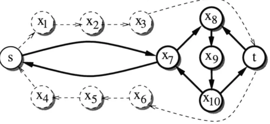
Figure 2-1: A sample graph for 2-SCSS, with terminals s and t. The optimal subgraph is in solid lines.
Figure 2-1 illustrates some of the difficulties of this problem. Let s, t be our
terminals. The optimal subgraph consists of the six nodes sX 7, , x8 9, xio, t. The
paths from s to t and t to s share vertex x7, and share the vertex sequence x8 -+
-g - x1o. Note that the optimal subgraph includes neither the shortest path from s
2.1
The token game
To compute the optimal subgraph H, we will place two tokens, called
f
and b, on vertex s. We then move the tokens along edges,f
moving forward along edges, and b moving backwards along edges, until they both reach t. Then the set of nodes visitedduring the sequence of moves will contain paths s --+ t and t -~> s.
To find the smallest subgraph H containing those paths, we will charge for the moves. The cost of a move will be the number of new vertices entered by the tokens during that move. Clearly we could never find a move sequence that gets both tokens from s to t with cost lower than HJ - 1, the size of the optimal solution H minus one
(since we never charge for s). In fact, we will show that the lowest cost move sequence to get the tokens from s to t will have cost exactly JH - 1, and thus corresponds to an optimal solution.
The three kinds of moves we allow are given below. The notation (x, y) refers to the situation where token
f
is on vertex x, and token b is on vertex y. The expression"(x1, Y1) 4 (x2, Y2)" means that it is legal to move token
f
from x1 to x2, and tokenb from yi to Y2 (at the same time), and that this move has cost c. We want to find a move sequence from (s, s) to (t, t) with minimal cost.
(i) Token
f
moving forward: For every edge (u, v) E E and all x E V, we allow(a) the move (u, x)
-4
(v, x), and(b) the move (u, v) + (v, v).
(ii) Token b moving backward: For every edge (u, v) E E and all x E V, we allow (a) the move (x, v) + (x, u), and
(b) the move (u, v)
-+
(u, ).(iii) Tokens switching places: For every pair of vertices a, b E V for which there is a path from a to b in G, we allow the move (a, b) 4 (b, a), where c is the length of the shortest path from a to b in G. By length we mean the number of vertices besides a and b on that path.
Type (i) and (ii) moves allow the tokens
f
and b to move forward along a single edge, and backward along an edge, respectively. Usually the cost is 1, accounting for the new vertex that the token visits. Only in the case where a token reaches a vertex with a token already on it, the cost is 0, since no 'new' vertices are visited.Type (iii) moves allow the two tokens to switch places. We call this type of move a "flip", and say that the vertices on the shortest path from a to b are implicitly traversed by the tokens. The cost c of the move accounts for all of these vertices.
lowest cost way to move both tokens from s to t is the following (we use subscripts to denote the type of the move).
(s, s)
-4
() (x7, s) (ii) 0 (x7, x7)-4
() (x8, x7)-4
(x8, xio)A
(X10,x8)4
(xio, t)A
(t, t)(ii) (iii) (ii) (W
The weight of this sequence is 5, which is JHJ - 1, and the nodes visited by the tokens are exactly the nodes in the optimal solution H.
2.2
The Algorithm
Let us phrase the preceding discussion in an algorithmic form. To compute H, we first construct a 'game-graph' G. The nodes of the graph correspond to token positions (x, y), the edges to legal moves between positions. In our case, the nodes are just
V x V, and the edges are the ones given above as legal moves.
Finding H is done by computing a lowest cost path from (s, s) to (t, t) in G. The graph H then consists of all the vertices from V that are mentioned along that path, including the vertices that are implied by type (iii) moves.
Running time: Clearly, this game-graph can be computed in polynomial time. First, we do an all-pairs-shortest-paths computation on G to obtain the information we need to set up the type (iii) moves. This takes time O(mn) using breadth-first search, where n and m are the number of vertices and edges in the original graph
G. Then, we add to G all the edges corresponding to legal moves one at a time.
The number of vertices in G is O(n2). The number of type (i) and type (ii) edges in
G is O(mn), since there is a type (i) and type (ii) move for every edge and vertex
combination in G. The number of type (iii) edges is O(n2) making the total time to compute G equal to O(mn).
Now we just have to perform a single-source shortest paths computation from (s, s) to obtain H. Since we now have weights on the type (iii) edges, we cannot use breadth-first search. For a simple implementation, we could use Dijkstra's algorithm (which
has a running time of O((V|2)), and achieve a running time of O(n'). Using Fibonacci
heaps [FT87], which performs single-source shortest paths in time ( E + IV log V),
we achieve a running time of O(mn + n2 log n).
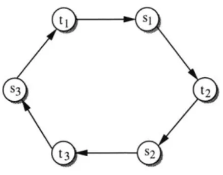
As an aside, this algorithm can also be used to solve 2-DSN. Given a graph G and two node-pairs (s, t,), (s2, t2), add two nodes s, t and edges s -+ si, ti -+ t, t -+ s2, t2 -+ s to the graph and solve 2-SCSS for the two terminals s, t. The solution for this problem is also an optimal solution for the original 2-DSN problem (if we omit s and t). This leads to a running time of ((mn + n2 log n) for 2-DSN, which is the same as the running time obtained by Natu and Fang [NF95].
In fact, we can do a little better for the unweighted case using more complicated shortest paths algorithms. For a more detailed analysis, see Appendix A.2.
2.3
Correctness
The proof that our algorithm actually solves 2-SCSS can be split into two claims. We provide a proof here that motivates the techniques used in the general case. An
alternate proof can be found in [NF95, NF97]. Claim 2.3.1
If there is a legal move sequence from (s, s) to (t, t) with cost c, then there is a
subgraph H of G of size < c + 1 that contains paths s -- t, and t - s.
If we follow a move sequence from (s, s) to (t, t), then f and b trace out paths
s ---* t and t -- s, and this becomes our solution H. Moreover the tokens traverse at
most c + 1 vertices, since each vertex (except s) that we visit adds one to the cost of the move sequence.E
Claim 2.3.2
Let H* be an optimal subgraph containing paths s -,-- t and t - s. Then there exists
a move sequence from (s, s) to (t, t) with total cost
IH*I
- 1.This is the more difficult part of the correctness proof. We can prove it by actually
constructing a move sequence (s, s) -+ (t, t), using H* as a 'map.'
When moving the tokens from (s, s) to (t, t), we 'pay' each time we reach a new vertex in H*. In order to achieve total cost IH*I - 1 we must make sure that we pay only once for each vertex in H*. To ensure this, we enforce one rule: after a token moves off a vertex, no other token will ever move to that vertex again. We say that a vertex becomes 'dead' once a token moves from it, so that tokens are only allowed to move to vertices in H* that are 'alive'. Note that the notion of dead and alive vertices is only used for the analysis, the algorithm itself never explicitly keeps track of them.
As we construct the move sequence, we maintain the invariant that there exist paths of 'alive' vertices from the position of token
f
to t, and from t to the position of token b. This will make sure that we do not have to violate our rule to proceed with the sequence. When we reach (t, t), we will have constructed a legal move sequence, and paid for each vertex inIH*
at most once. This will immediately imply the claim. We construct the sequence in a greedy fashion. We start at position (s, s), and perform the following steps:(a) Move token
f
with type (i) moves. Choose some path in H* from the position of tokenf
to t. We move tokenf
forward along edges in that path (killing vertices along the way) using type (i) moves, until we reach t, or we reach a node x where moving tokenf
would leave token b stranded; i.e., all paths of alive vertices from t to the position of token b go through x. We cannot move tokenf
off of x, otherwise we would kill x and lose our invariant that there is a path of alive vertices from t to the position of token b (see figure 2-2).(b) Move token b with type (ii) moves. Choose some path of alive vertices from t to the position of token b, and move the token b backwards along edges of that path towards t using type (ii) moves. We proceed until we reach t, x, or some node y
$
x that would leave the tokenf
stranded if we killed it (all paths from x to t go through y).If the tokens are both on t, we are done. If the tokens are now on the same node x, go back to step (a). Note that in both these cases the last move of token b was free. If token b reached some node y
$
x, we have a 'deadlock' (see figure 2-2). (c) Resolve the deadlock with a flip: a type (iii) move. To resolve thedead-lock, we will use a type (iii) move. We know that all paths from x to t go through y, so there must be two disjoint simple paths Px, and Pyt in H* (see figure 2-2). Also, since all paths from t to y go through x, there must be a simple path Px. Path Ptx must also be disjoint from Pxy, since if it were not, token b would be able to get from y to t without going through x.
We apply the type (iii) move (x, y) -+ (y, x). The cost of the move is at most the size of P y (not including x and y) and we only kill nodes on Pxy. Since Pxy is disjoint from both Ptx and Pyt, we maintain our invariant that there are paths of 'alive' vertices from the position of token
f
to t and from t to the position of token b. Go back to step (a).token f p token b
x t
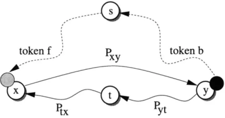
Figure 2-2: Deadlock in the construction of an optimal move sequence. Token
f
has moved forward onto node x, and token b has moved backward onto node y. All paths from x to tgo through y, and al paths from t to y go through x. Therefore, moving either one of the tokens individually would leave the other token stranded. We resolve this deadlock using a flip: a type (iii) move exchanging the positions of the tokens.
We never move a token onto a dead vertex, and each step maintains the invariant that there are paths of alive vertices from the position of token
f
to t and from t to the position of token b. Therefore both tokens reach t, and we only pay once for each vertex we visit. Since we only visit vertices in H*, and we don't pay for s, it must be the case that the cost of the move sequence is at mostIH*J
- 1.EThis claim immediately implies that the shortest path in d will correspond to an optimal solution, since by Claim 2.3.1 and the minimality of H* there are no paths
in G on length less than IH*| - 1.
The token movements for the p = 2 case essentially describe the way in which paths are shared in the optimal solution. Path sharing for p > 3 is more complex, so we will need a richer set of token moves, and a much more involved proof.
Chapter 3
Strongly Connected Steiner
Subgraphs
In this chapter we give an algorithm for p-SCSS, which is a generalization of the algorithm for 2-SCSS given in the previous chapter.
Again we will use token movements to trace out the solution H. The way the tokens move is motivated by the following observation. Consider any strongly con-nected H containing
{s,...
,s1,}. This H will contain paths from each s1,... 7sP1to sp, and these paths can be chosen to form a tree rooted at sp; we will call this tree the forward tree. The graph H will also contain paths from s, to each s,...s_1 forming what we call the backward tree. Moreover, every H that is the union of two such trees is a feasible solution to our p-SCSS instance.
For ease of notation, we set q := p - 1 for the remainder of this chapter, and let r := s,, as s, plays the special role of 'root' in the two trees.
3.1
Token moves for p-SCSS
To trace out the two trees, we will have q "F-tokens" moving forward along edges in the forward tree from {s1,..., Sq} to r, and q "B-tokens" moving backward along
edges from {s1,..., Sq} to r. Given a set of legal moves, we will again look for the
lowest cost move sequence that moves all tokens to r. This will then correspond to
the smallest subgraph containing paths si --+ r and r -* si for all i < q, which is the
graph we are looking for.
Since both sets of tokens trace out a tree, once two tokens of the same kind reach a vertex, they will travel the same way to the root. In that case, we will simply merge them into one token. It is therefore enough to describe the positions of the tokens by a pair of sets (F, B), where F and B are the sets of nodes currently occupied by the F- and B-tokens.
Again, we have three types of legal token moves. Type (i) moves correspond to F-tokens moving forward along an edge, and type (ii) moves correspond to B-tokens moving backward along an edge. We do not charge for entering a vertex if another token is already on it.
F' B F' F'
B b
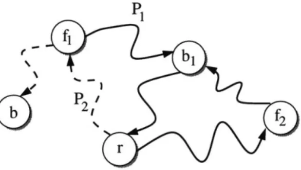
Figure 3-1: Flipping f and b, with tokens F' and B' that need to be "picked up." The black nodes are the set M.
Since there are are at most q tokens of each type, the possible token positions for a particular type are the subsets of V of size at most q. So, let Pq(V) be the set of subsets of V of size at most q.
(i) Single moves for F-tokens: For every edge (u, v) E E, and all token sets F E Pq(V), B E Pq(V), such that u E F, the following is a legal move:
(F, B) 4 ((F \ {u}) U {v}, B)
where the cost c of the move is 1 if v V F U B, and 0 otherwise.
(ii) Single moves for B-tokens: For every edge (u, v) E E, and all token sets F E
Pq(V), B E Pq(V), such that v E B, the following is a legal move:
(F, B) 4 (F, (B \ {v}) U {u})
where the cost c of the move is 1 if u V F U B, and 0 otherwise.
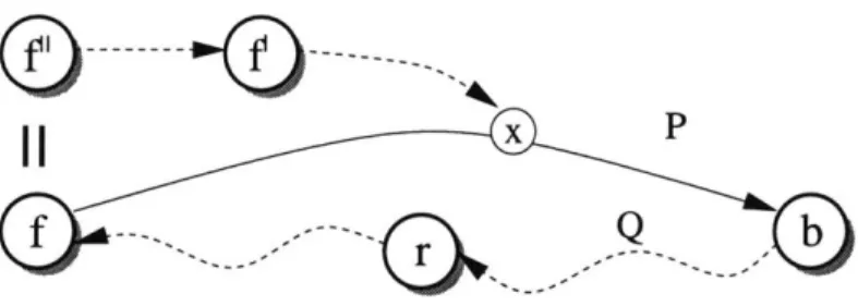
Type (iii) moves allow tokens to pass each other, similar to the type (iii) moves in the previous chapter, except that this time the "flip" is more complex (see figure
3-1). We have two 'outer' tokens,
f
and b, trying to pass each other. Betweenf
andb there are other F-tokens moving forward and trying to pass b, and B-tokens moving
backward and trying to pass
f.
These tokens, sitting on node sets F' and B', are 'picked up' during the flip.(iii) Flipping: For every pair of vertices
f,
b, vertex sets F, B, F' c F, B' c B, suchthat:
" f E F E Pq(V)
*
f E B C Pq(V)" there is a path in G from f ---> b going through all vertices in F' U B'
the following is a legal token move:
(F, B) ((F
\ {f} \
F') U {b}, (B\
{b}\
B') U{f})
where M is the set of vertices on a shortest path from
f
to b in G going through all vertices in F' U B', besides f,b and the vertices in F' U B'.3.2
The algorithm for p-SCSS
We can now state the algorithm for p-SCSS:1. Construct a game-graph d = (V, E) from G = (V, E). Set V := Pq(V) x Pq(V), the possible positions of the token sets, and F := all legal token moves defined above.
2. Find a shortest path P in d from ({s1,... , },{S1,..., Sq}) to ({r}, {r}).
3. Let H be the union of {s,..., s, r} and all nodes given by P (including those in sets M for type (iii) moves).
The difficult part of constructing the game-graph d is computing the costs for the type (iii) moves that flip
f
and b. We need to know the size of shortest path betweenf
to b in G going through all vertices in F'UB'. Note that we do not require this path to be simple. So, if we knew the order in which the vertices in F' and B' occurred on the path, computing the shortest path becomes easy: it is just the union of the shortest paths between consecutive nodes in that order. Since the number of tokens in F'U B' is bounded by 2(q - 1), which is a constant, we can simply try all possible permutations of the nodes in F' U B'.The total running time of the algorithm is O(n2p-). This can be improved slightly
if the graph is sparse (m = O(n log n)). For more details on the running time, see appendix A.2.
3.3
Example
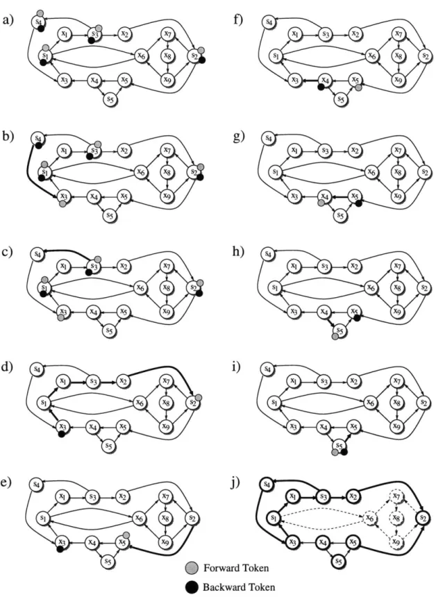
As an example we look at how the token game works on the graph in figure 3-2. Our terminals are si, s2, s3, s4, S5, and so we set s5 to be the root vertex, and put a forward
and backward token on each of the other terminals (figure 3-2(a)). In figures 3-2(b-i) we see the following move sequence:
{si, s2, s3, .S4}, {S1, S2, s3, 84})
-4
({s, S2, S, X3}, {1 , 82, S3, S4}) (i)4
({sI, s2, s3, X3}, {si, 82, S3}) ({S2}, {x 3}) () (iii)4
({X5}, {X3} h1 ({xo}, {x34}4
({X4}, {XS})4
({s5}, {Xs})4
({ss}, {ss}). (i) (ii)The total cost of the moves is 6, and therefore equal to Hj - q = 10 - 4 = 6, as
XI s{ X2 X7 S1x6 X8 s2 X3 X4 X5 X9 s5 XI s3 X2 X7 si 6 X8 X3 4 X5 X9 S5 X1 s3® X2 X7 s1 x6 X8 X3 4 X5 X9 S5 XI s3 X2 X7 X3 4 X5 X9 s5 e) Dn ~orw f) S4 X1 S3 X2 X7 X3 4 X5 X9 S5 g) S4 XI s3 X2 X7 s1 x6 X8 s2 X3 4 X5 X9 S5
h)
s4 XI s3 X2 X7 s1 x6 X8 s2 X3 X4 X9 S5 XI s3 X2 X7 s1 x6 X8 S2 X3 X4 X5 X9 XI S3 2 4 X7 X3 X4 59 * Backward TokenFigure 3-2: An example for the p-SCSS algorithm. Bold lines indicate the path of the last token move.
of the terminals {si, S2, S3, 84, 5}, the nodes {x3, x4, x5} mentioned in the sequence
of moves, and the nodes {x1, X2} in the set M for the first type (iii) move. This is
optimal.
3.4
Correctness of the p-SCSS algorithm
The correctness proof for our p-SCSS algorithm can be split into the same two parts we used for 2-SCSS.
Lemma 3.4.1
Suppose there is a move sequence from ({si, . . , sq}, {si,... , Sq}) to ({r}, {r}) with
total cost c. Then there exists a solution H to this p-SCSS instance of size < c + q. Moreover, given the move sequence, it is easy to construct such an H.
Proof: This follows directly from the definition of the moves. The cost of any move sequence is an upper bound on the number of vertices traversed by that sequence. Given the constructive nature of the moves, it is also easy to actually find H. U
Together with the following, much more involved lemma, the correctness of the algorithm is proved.
Lemma 3.4.2
Suppose H* = (V*, E*) is any minimum cardinality feasible solution. Then there is a move sequence from ({si, ... ,sq}, {8i,... , Sq}) to ({r}, {r}) with weight equal to
|H*| - q.
Proof: To prove this lemma, we will effectively construct such a move sequence, where all intermediate positions of the tokens will be in H*.
When moving the F- and B-tokens from {si,..., Sq} to r, we 'pay' each time we
reach a new vertex. To account for each move, and achieve total cost
|H*
- q, we will use the same method as we used for 2-SCSS. We enforce the same rule: after a token moves off a vertex, no other token will ever move to that vertex again. As before, we say that a vertex becomes 'dead' once a token moves from it, so that tokens are only allowed to move to vertices in H* that are 'alive'. This also makes sure that our move sequence will be finite, since no token can return to a vertex it has already visited.We say that a token t requires a vertex v E V* if all legal paths for t to get to r pass through v. By 'legal paths' we mean paths that are within H*, go in the appropriate direction for the token t, and do not include any dead vertices. We will sometimes speak of tokens requiring tokens; in this case we mean that the first token requires the vertex on which the second token is sitting. Note that the requirement relation among tokens moving in the same direction is transitive, i.e. if fi requires
f2, and f2 requires x, then fi also requires x.
We will construct our move sequence in a greedy fashion. That is, we will move tokens towards r using type (i) and (ii) moves, until each token sits on a vertex that is required by some other token to get to r. In this case we cannot apply any more type
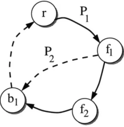
Figure 3-3: Showing Claim 3.4.4, that all tokens that require a vertex on P are on P themselves.
(i) or (ii) moves - doing so would leave another token stranded as it is not allowed to move onto the then dead vertex.
In this case we need to use a type (iii) move to resolve the deadlock. Showing that this is always possible is the core of the correctness proof, the 'flip lemma' shown in Section 3.5. To state this lemma and see how it implies the correctness of the algorithm, we have to introduce some additional notation.
Let the 'Fo-tokens' be the F-tokens that are not required by any other F-token. Similarly, let the 'Bo-tokens' be the B-tokens that are not required by any other B-token.
Lemma 3.4.3 (The Flip Lemma)
Suppose every token is required by some other token. Then there is an FO-token f and a BO-token b such that
*
f requires b, and no other FO-token requires b,* b requires f, and no other BO-token requires f. El
We will prove this lemma in the next section. Let us now see how it concludes the proof of Lemma 3.4.2.
Let
f
and b be chosen according to the Flip Lemma. Fix any simple path from f to r that uses only live vertices. Call P the portion of this path betweenf
and b, andQ
the portion between b and r (see figure 3-3). By definition, P andQ
are disjoint. Claim 3.4.4All tokens that require a vertex on P are on P themselves.
Proof: We prove the claim for F-tokens; a symmetric argument applies to B-tokens. Suppose some F-token
f' $ f
requires a vertex x on P. Every path x -+ r mustinclude b, otherwise
f
could move to x, and then to r, without visiting b. Therefore,f'
also requires b (see figure 3-3). The tokenf'
cannot be an FO-token, since the Flip Lemma tells us thatf
is the only Fo-token that requires b. Note that due to transitivity, every F-token is either an FO-token, or required by some FO-token, sof
must be required by some FO tokenf".
By transitivity,f"
requires b, and so f" = ,by the Flip Lemma.
---Since
f
=f"
requires f', the tokenf'
is either on P orQ.
Iff'
is onQ,
then x is also onQ,
since f' requires x. This contradicts the fact that P andQ
are disjoint, and sof'
must be on P. ULet F' be the set of F-tokens that are on the path P, and B' be the set of B-tokens on P. We can apply a type (iii) move that switches
f
and b, and picks up F' and B' along the way. All vertices on P become dead. No token is stranded, since by Claim 3.4.4, all tokens that required a vertex on P were on P, and therefore were picked up by the flip.We have shown, pending the Flip Lemma, that each step of the construction of our move sequence preserves paths of 'alive' vertices from the F-tokens to r and from
r to the B-tokens, and never moves a token onto a dead vertex. This shows that we can always continue the construction of our move sequence until all tokens reach r,
and that the cost of the move sequence will be no more than IH*| - q. U
3.5
The Flip Lemma
To complete the proof of correctness, it remains to show Lemma 3.4.3, the Flip Lem-ma. We prove the Flip Lemma by making a graph out of the requirement relationships between the FO and BO tokens. We show that there is a two-cycle in this graph, con-sisting of an FO and a BO token, that does not have any other incoming requirements. This proves the lemma.
During the discussion, keep in mind that transitivity only holds among require-ments for the same type of token; if an F-token
f
requires a node (or a token) x, and some F-tokenf'
requiresf,
then f' requires x. However, if some B-token b requiresf,
it is not necessarily the case that b requires x, since b is moving backwards along edges. Proof of Lemma 3.4.3 (The Flip Lemma):The requirement graph Greq. Let Greq = (Vreq, Ereq) be a new directed graph,
whose nodes are the FO and BO-tokens. The edges in Ereq correspond to requirements:
Greq has an edge x -+ y iff the token x requires the token y.
This graph has a lot of structure. First of all, Greq is bipartite, since no two FO-tokens (and no two Bo-tokens) require each other (by the definition of an Fo- and Bo-token). For the remainder of the discussion, we will use
f
to denote a node on the FO side of the bipartition, and b to denote a node on the BO side.By assumption (every token is required by some other token) and by definition (an FO-token is not required by any F-token), we know that every FO-token is required by at least one B-token. We know that either that B-token is a BO-token, or there is another BO-token that requires that B-token. Therefore, by transitivity for B-tokens, every FO-token is required by at least one BO-token. By symmetry, every Bo-token
is required by at least one FO-token. Therefore, every node in Greq has at least one incoming edge.
We want to find a two-cycle in Gre, with no incoming edges, since two tokens in a such a cycle would require each other, but would be required by no other tokens, and the lemma would be proven. We can view Geq as a dag (directed acyclic graph) of strongly connected components, and sort the strongly connected components topo-logically. Let C be the first component in that ordering. This means that no token outside of C requires any token in C. Furthermore, C cannot consist of only one node, since then that token would be required by no other token, in contradiction to our assumption that every token is required by at least one token. If C contains exactly two nodes, we have found our two-cycle.
We will prove that C cannot consist of more than two nodes, which will imply the Flip Lemma, and the correctness of our algorithm. The proof rests on the observation that Geq satisfies a kind of transitivity, which we call the projection property. After showing his property, we prove the claim by contradiction by applying the projection property across the requirement graph.
Claim 3.5.1
Projection: Suppose for three nodes f1, f2, b1 (f1
#
f2) in Gre, we have edges f1 - b1and b1 -+ f2 in Greq. Then the following holds: all nodes b that have an edge b -+ f1
also have an edge b -+ f2.
e b,
r
Figure 3-4: Proving the projection property in Greq. The solid lines are paths in H* corresponding to edges fi -+ b1 and b1 -+ f2 in Greq, the dashed line to the edge b -+
fi.
Proof: By definition of FO, there is a legal path in H* from fi to r avoiding f2. Since
fi
requires bl, this path goes through bi. Therefore, there is a path P from fi to b1avoiding f2 (see figure 3-4).
Suppose that some node b in Geq has an edge b -+ fi. We show that b -+ f2 is
also in Gre, by contradiction. If b -+ f2 is not in the requirement graph, then there is
a legal path in H* from r to b avoiding f2. Since b requires fi, this path goes through
fi.
Therefore, there is a path P2 in H* from r to fi avoiding f2. Combining P2 and P1, we obtain a path from r to b, that does not visit f2 in contradiction to b1 -+ f2A symmetric property holds by exchanging f's and b's, i.e. for any triple fi, bl, b2,
if there are edges b1 -+ fi and fi -+ b2 in Greq, then for every node f in Greq, if there is an edge
f
-+ bi, then there must also be an edgef
-+ b2-The projection property has a profound effect on the structure of Greq. In fact, it shows that if there is a path in Geq from a node b to a node
f,
then there is an edge from b tof.
To see this, consider the last four nodes on the path from b tof
in Greq,b" -+
f'
-+ b' -f.
By projection, there must be an edge b" -+f.
This shortens thepath by two. This argument can be continued up the path until it shows that there
must be an edge b -+
f.
A symmetric argument (using the symmetric projection property) shows that if there is a path in Geq from a node f to a node b, then there is an edge from f to b. We further conclude that every strongly connected component in Greq is a complete bipartite graph (every pair of nodes on opposite sides of the bipartition is connected in both directions). Now we are ready to finish the Flip Lemma.
Claim 3.5.2
No strongly connected component C of Greq has more than 2 nodes.
Proof: We prove the claim by contradiction. Assume that a strongly connected component C in Greq has at least three elements. Either there are two FO nodes in
C, or two BO nodes in C. We assume there are two FO nodes (a symmetric argument
shows the other case). Since C is a complete bipartite graph, there must be a complete bipartite subgraph of C consisting of nodes fi,bi,f2.
r P1
P fi
2
,.-22
Figure 3-5: Components with more than 2 elements are impossible
We turn back to H* to show that this structure cannot exist. Since b1 requires
both fi and f2, there is a legal path in H* from r to b1 that visits both fi and f2
(solid lines in figure 3-5). Without loss of generality assume that fi is the first node on that path, so that there is a path P from r to fi that avoids f2. Since fi requires
bi, but fi does not require f2, there must also be a path P2 from fi to b1 that avoids
f2 (dashed lines in figure 3-5). Combining P and P2, we obtain a legal path in H*
from r to b1 that avoids f2, in contradiction to the fact that b1 requires f2.
Chapter 4
The Directed Steiner Network
problem
4.1
The Algorithm
In this chapter we show how to apply the algorithm developed in the previous chapter
to solve DIRECTED STEINER NETWORK problem (p-DSN), for any constant p.
DIRECTED STEINER NETWORK (p-DSN) (unweighted, node-minimizing): Given a
directed graph G = (V, E), and p pairs of nodes in the graph {(Si, ti),..., (s, tp)}, find the subgraph H of G with the fewest number of nodes that contains paths from si to tj for 1 < i < p.
We use the same general model of a token game, but now we have tokens moving from each source si to its destination ti. This time, we have no backwards moving tokens, and also tokens do not merge when they reach the same node. We describe
the positions of the tokens by a p-tuple (fi, f2, ... , f,). We have two kinds of moves
for the tokens. The first kind of move allows a single token to move one step along an edge.
(i) For each edge (u, v) we include the moves (-, u, -) - (-, v, -), meaning that one token moves from u to v, and all others remain where they are. The cost c of the move is 0 if v already has a token on it, and 1 otherwise.
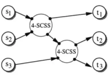
We also allow a group of tokens to move through a strongly connected component all at once. To see why this is useful, consider the optimal solution to p-DSN and contract every strongly connected component into a single node; the resulting graph is a dag (see figure 4-1). Each contracted component has at most p tokens entering, and at most p tokens exiting. We can compute the best way for some group of k tokens (k < p) to move from any k or fewer specific entrance points to any k or fewer specific exit points in a strongly connected component by solving an instance of 2k-SCSS.
4-SCSS
S2 t2
4-SCSS s3
Figure 4-1: A solution to p-DSN is a dag of strongly connected components
(ii) For all k < p, and for every set of k node-pairs {(fi, x1), (f2, x2), .- -, (fk, Xk)},
for which there is a strongly connected subgraph of G containing all of the nodes in the pairs, we allow the move
( f-f2--.- -fk-)
4 (- 1- -2 ..
-Xk-)-The cost c of this move is the size of the smallest strongly connected component
containing the vertices {fi, f2, ...
f,
kX 1, X2, ... , Xk} minus the size of the set {fi, ... , fk}. We can use the the algorithm developed in Chapter 3 to computethis cost.
Similar in structure to our algorithm for p-SCSS in Chapter 3, the algorithm for
p-DSN consists of the following steps.
1. Compute the game-graph g, where the vertices in g are p-tuples of vertices in the input graph G, and edges are included for each legal token move.
2. Find the minimum-weight path P in g from (si, ... , s,) to (ti,..., t,). 3. Output the subgraph H of G induced by P, i.e. the subgraph containing
" all vertices of G explicitly 'mentioned' by vertices in P, and
" for all type (ii) moves used in P, all the vertices making up the smallest
strongly connected component containing the fi's and xi's used to define that move.
4.2
Correctness
As for the previous algorithms, it is easy to see that for any move sequence from
(Si,... , s,) to (ti, ... , t,) of cost c, there is a feasible solution H of size at most
c + 1{s1,... , sp}1. It is also easy to find this H, given the move sequence. The