Raindrop size distributions and radar reflectivity?rain rate relationships for radar hydrology

HAL Id: hal-00304636

https://hal.archives-ouvertes.fr/hal-00304636

Submitted on 1 Jan 2001

HAL is a multi-disciplinary open access archive for the deposit and dissemination of sci-entific research documents, whether they are pub-lished or not. The documents may come from teaching and research institutions in France or abroad, or from public or private research centers.

L’archive ouverte pluridisciplinaire HAL, est destinée au dépôt et à la diffusion de documents scientifiques de niveau recherche, publiés ou non, émanant des établissements d’enseignement et de recherche français ou étrangers, des laboratoires publics ou privés.

rate relationships for radar hydrology

R. Uijlenhoet, J. H. Pomeroy

To cite this version:

R. Uijlenhoet, J. H. Pomeroy. Raindrop size distributions and radar reflectivity?rain rate relationships for radar hydrology. Hydrology and Earth System Sciences Discussions, European Geosciences Union, 2001, 5 (4), pp.615-628. �hal-00304636�

Raindrop size distributions and radar reflectivity–rain rate

relationships for radar hydrology

*

Remko Uijlenhoet

1

Sub-department Water Resources, Department of Environmental Sciences, Wageningen University and Research Centre, Wageningen, The Netherlands; also Laboratoire d’étude des Transferts en Hydrologie et EnvironnementUMR 5564, CNRS-INPG-IRD-UJF, Grenoble, France

Email: [email protected]

Abstract

The conversion of the radar reflectivity factor Z (mm6 _m-3_{) to rain rate R (mm h}-1_{) is a crucial step in the hydrological application of weather}

radar measurements. It has been common practice for over 50 years now to take for this conversion a simple power law relationship between

Z and R. It is the purpose of this paper to explain that the fundamental reason for the existence of such power law relationships is the fact that Z and R are related to each other via the raindrop size distribution. To this end, the concept of the raindrop size distribution is first explained.

Then, it is demonstrated that there exist two fundamentally different forms of the raindrop size distribution, one corresponding to raindrops present in a volume of air and another corresponding to those arriving at a surface. It is explained how Z and R are defined in terms of both these forms. Using the classical exponential raindrop size distribution as an example, it is demonstrated (1) that the definitions of Z and R naturally lead to power law Z–R relationships, and (2) how the coefficients of such relationships are related to the parameters of the raindrop size distribution. Numerous empirical Z–R relationships are analysed to demonstrate that there exist systematic differences in the coefficients of these relationships and the corresponding parameters of the (exponential) raindrop size distribution between different types of rainfall. Finally, six consistent Z–R relationships are derived, based upon different assumptions regarding the rain rate dependence of the parameters of the (exponential) raindrop size distribution. An appendix shows that these relationships are in fact special cases of a general Z–R relationship that follows from a recently proposed scaling framework for describing raindrop size distributions and their properties.

Keywords: radar hydrology, raindrop size distribution, radar reflectivity–rain rate relationship

Introduction

Because rainfall constitutes the main source of water for the terrestrial hydrological processes, accurate measurement and prediction of the spatial and temporal distribution of rainfall is a basic issue in hydrology. As a result of the gradual development of radar technology over the past 50 years, ground-based weather radar is now finally becoming a tool for quantitative rainfall measurement instead of merely for qualitative rainfall estimation. Potential areas of application of ground-based weather radar systems in operational hydrology include storm hazard assessment and flood forecasting, warning, and control (Collier, 1989). The current attention for land surface hydrological processes in the climate system has stimulated research into the spatial

and temporal variability of rainfall as well. A potential area of application of ground-based weather radar in this context is the validation and verification of sub-grid rainfall parameterisations for atmospheric mesoscale models and general circulation models (Collier, 1993).

A fundamental problem before radar-derived rainfall amounts can be used for hydrological purposes is to make sure that they provide accurate and robust estimates of the spatially and temporally distributed rainfall amounts. The branch of hydrology dealing with this problem is now starting to be known as radar hydrology. The crucial step in tackling the so-called observer’s problem associated with radar remote sensing of rainfall is the conversion of the radar reflectivities measured aloft to rain rates at the ground. The exact manner in which this conversion is carried out will obviously affect the precision of the radar rainfall estimates so obtained. Various aspects of the associated assumptions, error sources and uncertainties are discussed by Zawadzki *This paper is based on a lecture presented at the CEC Advanced Study

Course Radar Hydrology for Real Time Flood Forecasting, held at the Water Management Research Centre, University of Bristol, UK, 23 June– 3 July 1998.

(1984), Andrieu et al. (1997), Creutin et al. (1997) and Wood

et al. (2000), among others.

At the heart of the problem of radar hydrology lies the conversion of the radar reflectivity factor Z (mm6 _m-3_{) to}

rain rate R (mm h-1_{). The former can, in principle, be inferred}

from conventional (so-called single-parameter) weather radar measurements, whereas the latter is the variable of interest to hydrologists. [Note: The treatment of multi-parameter (e.g. polarization diversity) weather radar is beyond the scope of this paper—see for example Illingworth

et al., 2000.] It has been common practice for over 50 years

now (Marshall and Palmer, 1948) to take a simple power law relationship between Z and R (see Smith and Krajewski (1993) for a recent perspective) for this conversion. It is the purpose of this paper to explain that the fundamental reason for the existence of such power law relationships is the fact that the radar reflectivity factor Z and the rain rate R are related to each other via the raindrop size distribution.

To this end, Z and R are first derived in terms of the raindrop size distribution. Subsequently, empirical Z–R relationships reported in the literature are discussed, followed by the parameterisation of two forms of the raindrop size distribution and the associated expressions for

Z and R. An interpretation of the coefficients of the resulting

power law Z–R relationships in terms of the parameters of the raindrop size distribution is provided after this. The same section also presents several concrete examples of consistent power law Z–R relationships. Concluding remarks are then presented. Finally, Appendix A is concerned with the implications of a recently proposed scaling framework to describe raindrop size distributions and their properties for the interpretation of the coefficients of Z–R relationships (Sempere Torres et al., 1994, 1998).

The definitions of radar reflectivity

and rain rate

RADAR REFLECTIVITY

The weather radar equation describes the relationship between the received power, the properties of the radar, the properties of the targets and the distance between the radar and the targets. In this treatment, the targets are assumed to be raindrops. At non-attenuated wavelengths, the weather radar equation becomes (e.g. Battan, 1973)

, 2 2 Z r K C Pr = (1)

where P (W) is the mean power received from raindrops_r

at range r (km), C is the so-called radar constant, K2 is a coefficient related to the dielectric constant of water (~ 0.93)

and Z (mm6 _m-3_{) is the radar reflectivity factor, hereafter}

simply referred to as radar reflectivity. All radar properties are contained in C, and all raindrop properties in K and2 Z. Z is related to the size distribution of the raindrops in the

radar sample volume according to (e.g. Battan, 1973)

( )

∫

∞ = 0 6_{N DdD,} D Z V (2)

where N_V

( )

DdD (the subscript V standing for volume) represents the mean number of raindrops with equivalent spherical diameters between D and D+dD (mm) present per unit volume of air. The corresponding units of NV

( )

D

are mm-1 _m-3_{. Hence, although Z is called the radar}

reflectivity factor, it is a purely meteorological quantity that is independent of any radar property. Because in practice the variations in radar reflectivity may span several orders of magnitude, it is often convenient to use a logarithmic scale. The logarithmic radar reflectivity is defined as

Z log

10 and is expressed in units of dBZ (e.g. Battan, 1973). Equation (1) can be used to convert weather radar measurements of the spatial and temporal distribution of the mean received power P to that of Z according tor

. 2 2 C K P r Z ₌ r (3)

Of course, estimates of Z obtained with this equation will only be perfect if the hypotheses on which it is based are satisfied. This implies among others a perfect radar calibration, Rayleigh scattering and the absence of attenuation, beam shielding and anomalous propagation. In reality, these conditions are hardly ever met, or one does not know definitely whether they are met. Therefore, in practice, one often speaks of the effective radar reflectivity factor Z_e in the context of Eqn. (3) (e.g. Battan, 1973). Nevertheless, even a perfect measurement of Z does not yet imply a perfect estimate of the rain rate R, as will be shown in the next section.

RAIN RATE

If the effects of wind (notably up and downdraughts), turbulence and raindrop interaction are neglected, the (stationary) rain rate R (in mm h-1_{) is related to the raindrop}

size distribution N_V

( )

D according to

( ) ( )

∫

∞ − × = 0 3 4 _, 10 6 D v D N DdD R π V (4)

where v

( )

D represents the functional relationship between the raindrop terminal fall speed in still air v (m s-1_{) and the}

equivalent spherical raindrop diameter D (mm). The simplest and most widely used form of the v

( )

D -relationship is the power law

( )

_D

_cD

γ

.

v

=

(5)

Atlas and Ulbrich (1977) demonstrated that Eqn. (5) with

778 . 3 =

c (if v is expressed in m s-1 _{and D in mm) and}

67 . 0 =

γ provides a close fit to the data of Gunn and Kinzer (1949) in the range 0.5≤ D≤5.0 mm (the diameter interval contributing most to rain rate). Although more sophisticated relationships have been proposed in the literature (e.g. Atlas

et al., 1973), it will be demonstrated later that the power

law form for the v

( )

D -relationship is the only functional form that is consistent with power law relationships between rainfall-related variables, notably between Z and R (Appendix A).

A comparison of Eqn. (4) with Eqn. (2) demonstrates that it is the raindrop size distribution N_V

( )

D (and to a lesser extent also the v

( )

D -relationship) that ties Z to R. This is why the analysis of raindrop size distributions and the associated Z–R relationships is of interest to hydrologists. In hydrological applications, it is clearly not the spatial and temporal distribution of Z that is of interest, but rather that of the rain rate R. A complicating factor is that the measurements of Z are made aloft, whereas estimates of R are generally at ground level. The difference between the value of Z aloft and that at the ground is determined by the

vertical profile of reflectivity (e.g. Andrieu and Creutin,

1995; Andrieu et al., 1995; Cluckie et al., 2000; Sanchez Diezma et al., 2000). Only at ranges close to the radar, where the height of the radar beam above the ground is small, can this factor be neglected. Even then, the time it takes the raindrops to fall from the radar sample volume down to the ground should often be taken into account.

Even if weather radar were to provide perfect measurements of the spatial and temporal distributions of Z at ground level, the radar rainfall measurement problem would not be solved completely. First of all, the relationship between the radar reflectivity factor Z and the rain rate R is generally not a unique relationship. Secondly, even if it were unique, it would generally be unknown. This fundamental uncertainty in the Z–R relationship provides a lower limit to the overall uncertainty associated with radar rainfall estimation. In the absence of any other error source affecting the radar estimation of Z, the rainfall measurement problem for single-parameter weather radar reduces therefore to optimally using the information Z is supplying about the raindrop size distribution for the estimation of R.

Empirical radar reflectivity-rain rate

relationships

On the basis of measurements of raindrop size distributions at the ground and an assumption about the v

( )

D -relationship (such as Eqn. (5)), it is possible to derive Z–R relationships (via regression analysis). There exists overwhelming empirical evidence (e.g. Battan, 1973) that such relationships generally follow power laws of the form

,

b

aR

Z

₌

(6)

where a and b are coefficients that may vary from one location to the next and from one season to the next, but that are independent of R itself. These coefficients will in some sense reflect the climatological character of a particular location or season, or more specifically the type of rainfall (e.g. stratiform, convective, orographic) for which they are derived.

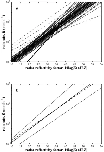
Battan’s (1973) standard treatise on radar meteorology quotes a list of 69 such empirical power law Z–R relationships derived for different climatic settings in various parts of the world (his Table 7.1, p. 90-92). Figure 1a provides all these relationships in one single plot. For reference, the linear Z–R relationship proposed by List (1988) for equilibrium rainfall conditions (which have been observed during ‘steady tropical rain’) is included as well. Figure 1b shows that, although there is an appreciable variability in the coefficients of these Z–R relationships associated with differences in rainfall climatologies, there seems to be a well-defined envelope comprising most relationships. A naive approach (taking the geometric mean of the individual prefactors a and the arithmetic mean of the exponents b – corresponding to averaging the linear

Z

log –log relationships) leads to the mean power lawR

relationship

. 238_R1.50

Z = (7)

Figure 1b compares this relationship with the most widely used Z–R relationship, 6 . 1 200R Z₌ (8)

(Marshall et al., 1955). The correspondence is close, particularly for rain rates between 1 and 50 mm h-1_{. This}

may be an explanation for the success of Eqn. (8) for many different types of rainfall in many parts of the world.

The question remains whether the coefficients a and b of the power law Z–R relationships are systematically different for different types of rainfall. Figure 2 shows a plot of b

versus a for Battan’s 69 Z–R relationships. On the basis of the remarks given by Battan (in his Table 7.1), it is possible to associate 25 of these Z–R relationships unambiguously with a particular type of rainfall. Using the same stratification as Ulbrich (1983), four of the relationships can be associated with ‘orographic’ rainfall, five with ‘thunderstorm’ rainfall, ten with ‘widespread’ or ‘stratiform’ rainfall, and six with ‘showers’. The remaining 44 relationships cannot be unambiguously associated with a particular type of rainfall, either because they correspond to mixtures of different rainfall types or because the rainfall type is not specified at all. Figure 2 provides some indication that the orographic and thunderstorm Z–R relationships form coherent groups in the

( )

a, -phase space. On average, orographic rainfallb

tends to be associated with smaller prefactors and larger

exponents, whereas for thunderstorm rainfall the opposite seems to be the case. For the Z–R relationships associated with the other rainfall types, it seems less obvious to make unambiguous statements about their positions in the

( )

a,b -phase space. A physical interpretation of the coefficients a and b in terms of the parameters of the corresponding raindrop size distributions may help to explain their variability.

Parameterisation of the raindrop size

distribution

THE EXPONENTIAL RAINDROP SIZE DISTRIBUTION

Since, according to Eqns. (2) and (4), both Z and R are related to the raindrop size distribution NV

( )

D , it should be possible to express a and b as functions of the parameters of N_V

( )

D . Although many different parameterisations for N_V

( )

D have been proposed in the literature, notably the gamma (Ulbrich, 1983) and lognormal (Feingold and Levin, 1986) forms, the exponential raindrop size distribution introduced by Marshall and Palmer (1948) has found the widest application. There exists empirical evidence showing that averaged raindrop size distributions indeed generally tend to the exponential form (Joss and Gori, 1978; Ulbrich and Atlas, 1998). Note that the exponential parameterisation will be used here merely as an example of a family of raindrop size distributions. A general approach to deriving Z–R

10 15 20 25 30 35 40 45 50 55 60 10−1 100 101 102 a

radar reflectivity factor, 10log(Z) (dBZ)

rain rate, R (mm h −1 ) 10 15 20 25 30 35 40 45 50 55 60 10−1 100 101 102 b

radar reflectivity factor, 10log(Z) (dBZ)

rain rate,

R

(mm h

−1

)

Fig. 1. (a) The 69 power law Z–R relationships Z = aRb _{quoted by}

Battan (1973, p. 90–92), including five deviating relationships (dashed lines), four of which have prefactors a significantly smaller than 100 and one of which has an exponent b as high as 2.87. The bold line indicates the linear relationship Z = 742R (List, 1988). (b) the mean of Battan’s relationships, Z = 238R1.50 _{(bold solid line),}

the reference relationship Z = 200R1.6 _{(Marshall et al., 1955, bold}

dashed line) and the envelope of 64 (the thin solid lines in (a)) of Battan’s 69 Z–R relationships (thin sold lines).

102 103 1 1.1 1.2 1.3 1.4 1.5 1.6 1.7 1.8 1.9 2 prefactor of Z−R relationship, a exponent of Z − R relationship, b

Fig. 2. The coefficients a and b of the 69 power law Z–R

relationships Z = aRb _{(with Z expressed in mm}6 _m-3 _{and R in mm h}-1₎

quoted by Battan (1973), stratified according to rainfall type: orographic (circles), thunderstorm (triangles), widespread/ stratiform (stars), showers (squares), no unambiguous identification possible (dots). The dashed line corresponds to the reference relationship Z = 200R1.6 _{(Marshall et al., 1955); the dash-dotted line}

corresponds to Marshall and Palmer’s (1948) relationship Z = 237R1.50_{, which almost equals the mean of Battan’s relationship, Z =}

relationships, independent of any assumption regarding the exact functional form of the raindrop size distribution, is presented in Appendix A.

In their classical paper, Marshall and Palmer (1948) proposed a simple negative exponential parameterisation for the raindrop size distribution NV

( )

D as a fit to filter-paper measurements of raindrop size spectra for rain rates between 1 and 23 mm h-1_,

( )

D N₀exp

(

D

)

,

N_V = −Λ (9)

where (mm-1 _m-3_{) is a shorthand notation for}

( )

₀

V

N and Λ (mm-1_{) is the slope of the N}

( )

_D

V -curve on a

semi-logarithmic plot. An alternative interpretation of Λ is the inverse of the mean diameter of raindrops present in a volume of air (Uijlenhoet and Stricker, 1999). Marshall and Palmer found that N was approximately constant for any₀

rain rate, , 10 0 . 8 3 0 = × N (10)

and that Λ decreased with increasing rain rate R (mm h-1₎

according to the power law . 1 . 4 −0.21 = Λ R (11)

Although the filter paper raindrop size measurements to which it was adjusted corresponded to rain rates not exceeding 23 mm h-1_{, the Marshall-Palmer parameterisation}

has been found to remain a realistic representation of averaged raindrop size distributions for much higher rain rates (e.g. Hall and Calder, 1993).

Marshall and Palmer’s exponential parameterisation for the raindrop size distribution bears a functional dependence on only one variable, namely the rain rate R. In accordance with the terminology introduced by Sempere Torres et al. (1994, 1998), this variable will be called the reference

variable. The fact that the effective number of degrees of

freedom of the raindrop size distribution equals one is fundamental to rainfall estimation using conventional (i.e. single-parameter) weather radar. If this were not the case then Z would never contain enough information about the raindrop size distribution to yield a one-to-one power law relationship with (i.e. a direct functional dependence on) R. For the concrete case of exponential raindrop size distributions of the form of Eqn. (9), the existence of such one-to-one power law Z–R relationships implies that either

0

N should be constant, or Λ should be constant, or both should be related to each other (or to R) via a power law. This point is elaborated further in Appendix A, where it is demonstrated that these considerations are not specific to

the assumption of an exponential raindrop size distribution, but in fact hold for any possible parameterisation. In the context of this paper, the exponential form is merely used as a convenient (and plausible) example.

AN ALTERNATIVE FORM OF THE RAINDROP SIZE DISTRIBUTION

The raindrop size distribution has been defined above as the mean number of raindrops in a particular diameter interval present per unit volume of air N_V

( )

D (mm-1 _m-3_).

However, there exists a second form of the raindrop size distribution, written here as NA

( )

D (the subscript A standing for area), which can be defined as the mean number of raindrops in a particular diameter interval arriving at a

surface per unit area and per unit time (Uijlenhoet and

Stricker, 1999). The corresponding units of NA

( )

D are

mm-1 _m-2 _s-1_{. The distinction between N}

( )

_D

V and NA

( )

D is

fundamental to a proper understanding of the concept of raindrop size distributions. Using the terminology of Smith (1993), NV

( )

D is the raindrop size distribution pertaining to the sample volume process and N_A

( )

D that pertaining to the raindrop arrival process.

If the effects of wind, turbulence and raindrop interaction are neglected, the relationship between N_A

( )

D and NV

( )

D in stationary rainfall becomes

( ) ( ) ( )

D vD N D,

NA = V (12)

or equivalently

( ) ( )

D vD N

( )

D

N_{V =} −1 _{A (13)}

(Uijlenhoet and Stricker, 1999). The fact that there exist two forms of the raindrop size distribution is recognized by anyone analysing raindrop size distributions measured with disdrometers or optical spectrometers. This is because what is measured by such ground-based devices is actually

( )

D

NA , whereas NV

( )

D is the traditionally desired form of

the raindrop size distribution. Hence, Eqn. (13) should be applied to convert the former to the latter.

In order to be able to derive the raindrop size distribution

( )

D

NA per unit area and per unit time corresponding to

Marshall and Palmer’s NV

( )

D -parameterisation, a

particular v

( )

D -relationship needs to be assumed. Substituting Eqns. (5) and (9) into (12) yields

( )

D cN₀D exp

(

D

)

.

N_A = γ −Λ (14)

0 N

As noted previously by Smith (1993), the original exponential distribution for the diameters of raindrops in a volume of air changes to a non-exponential gamma distribution for the diameters of raindrops arriving at a surface. At the same rain rate, the latter is shifted towards larger raindrop diameters with respect to the former (Uijlenhoet and Stricker, 1999).

RESULTING EXPRESSIONS FOR RADAR REFLECTIVITY AND RAIN RATE

A comparison of Eqns. (12) and (13) with Eqns. (2) and (4) shows that, in terms of the two forms of the raindrop size distribution discussed in the previous section, the definitions of the radar reflectivity factor Z and the rain rate R can be (re)written as

( )

∫

∞ = 0 6_{N DdD,} D Z V (15) and

( )

. 10 6 0 3 4 _{D N DdD} R

∫

A ∞ − × = π (16)

Hence, Z is most naturally defined in terms of NV

( )

D and

R in terms of NA

( )

D . This is because Z is a state variable and R is a flux variable (Uijlenhoet and Stricker, 1999). In general, state variables describe the amount of a certain raindrop property (in this case the 6th power of their diameter, proportional to the square of their volume) present per unit volume of air (i.e. they are concentrations). Flux variables describe the amount of a certain raindrop property (in this case their volume) arriving at a surface per unit area and per unit time (i.e. they are flux densities). State variables are scalar quantities, i.e. they do not have directions. Flux variables are vector quantities, i.e. they have directions (namely vertically downward in the absence of wind and turbulence).

For an exponential raindrop size distribution NV

( )

D in the air (Eqn. (9)) and the corresponding gamma raindrop size distribution NA

( )

D at the ground (Eqn. (14)), the definition of Z becomes

( )

7 7, 0Λ− Γ = N Z (17) and that of R

(

₄

)

( )_. 10 6 4 0 4

_γ

γ

π

_× − _{Γ + Λ}− + = c N R (18)

Here, Γ

()

⋅ denotes the gamma function (Γ

( )

7 =6!=720 and

(

4+

)

=14.78

Γ γ for γ =0.67). The raindrop diameter integration limits have been assumed to be zero and infinity, respectively. In other words, the effects of truncation of the raindrop size distribution (e.g. Ulbrich, 1985) have been disregarded.

Resulting power law relationships

INTERNAL CONSISTENCY OF PARAMETERI-SATIONS FOR RAINDROP SIZE DISTRIBUTION An important requirement of sets of power law relationships between rainfall-related variables is that they should be

consistent with each other. This means that power law

relationships between rainfall-related variables should satisfy the definitions of these variables in terms of the parameters of the raindrop size distribution. For example,

0

N –R and Λ–R relationships should, when substituted in the defining expression for R (Eqn. (18)), lead to R= R. This so-called self-consistency requirement has been considered explicitly by Bennett et al. (1984) and Uijlenhoet and Stricker (1999) for exponential raindrop size distributions, and in a much more general fashion, for any form of the raindrop size distribution, by Sempere Torres et

al. (1994, 1998). Appendix A provides a summary of the

latter approach. The derivation presented here follows the approach of Uijlenhoet and Stricker (1999).

In Marshall and Palmer’s (1948) parameterisation, N₀ is the constant 8.0 × 103 _mm-1 _m-3 _{(Eqn. (10)). Given values}

for the parameters c and γ, the only free variable left in Eqn. (18) is therefore Λ. This determines a particular Λ –R relationship and consequently an entire set of power law relationships between any pair of rainfall-related variables. The widely used Λ–R relationship proposed by Marshall and Palmer is Λ = 4.1R–0.21_{(Eqn. (11)). Does this power law}

relationship satisfy the self-consistency requirement? In other words, to what extent is it consistent with the definition of R in terms of N₀ and Λ (Eqn. (18)), and for which values of the parameters c and γ ?

Equation (18) can be inverted to yield an expression for Λ explicitly in terms of c, γ, N , and R. This yields0

(

)

[

_{6 10 4}

]

( ) 1/(4 ) 1/(4 )_, 0 4 / 1 4 γ γ γ γ π ₋ + + − + + Γ × = Λ c N R (19)

where the (rainfall-related) variable N has not been0

included between the square brackets to distinguish it from the parameters c and γ. Note that, for the special case of a constant N , Eqn. (19) defines a power law 0 Λ–R relationship

whose prefactor is entirely determined by the values of c, γ , and N , and whose exponent depends only on 0 γ .

However, even in the general case where N0 is not a

constant, e.g. if N₀ bears a power law dependence on R, Eqn. (19) will retain its validity. In that case, an appropriate

0

N –R relationship will have to be substituted for N in0

Eqn. (19) and the exponent of the resulting _{Λ–R relationship} will have to be changed accordingly (Appendix A). Substituting Atlas and Ulbrich’s (1977) values for c and

γ

(for the applied units: c=3.778 and γ =0.67) and Marshall and Palmer’s (1948) value for N0 into Eqn. (19) yields

. 23 . 4 −0.214 = Λ R (20)

This _{Λ–R relationship differs only little from that proposed} originally by Marshall and Palmer (Eqn. (11)), which is surprising given their entirely different methods of derivation. Equation (20) is the result of an analytical derivation based on a theoretical parameterisation for the raindrop size distribution, whereas Eqn. (11) is the result of a sort of regression analysis based on experimentally determined mean raindrop size distributions for a number of rain rate classes.

Although the small difference between Eqns. (11) and (20) falls entirely within the limits of uncertainty normally associated with this type of relationships, it shows that the latter is not entirely consistent with Atlas and Ulbrich’s (1977) raindrop terminal fall speed parameterisation (at least not for diameter integration limits of 0 and _∞). The coefficients of the power law v

( )

D -relationship that are consistent with Marshall and Palmer’s parameterisation for the raindrop size distribution (Eqns. (9)–(11)) can be obtained by forcing the coefficients of the general Λ–R relationship (Eqn. (19)) to be 4.1 and –0.21, respectively.

Assuming 3

0 =8.0×10

N mm-1 _m-3_{, this yields c = 3.25 and}

γ = 0.762 (for the applied units). These values for c and γ should be regarded as effective values, however, and should not be confused with values obtained from actual fits of Eqn. (5) to measurements of raindrop terminal fall speeds (such as the values given by Atlas and Ulbrich (1977)). The purpose of this exercise is merely to demonstrate one possible approach to correct for the lack of internal consistency in Marshall and Palmer’s parameterisation for the raindrop size distribution. Other (more plausible) approaches will be discussed later.

CONSISTENCY OF RADAR REFLECTIVITY–RAIN RATE RELATIONSHIPS WITH PARAMETERISATIONS FOR THE RAINDROP SIZE DISTRIBUTION

Substitution of 3

0 =8.0×10

N mm-1_m-3 _{and Λ = 4.1R}–0.21

mm-1 _{into Eqn. (17) yields} ,

296_R1.47

Z ₌ (21)

an expression reported by Marshall and Palmer (1948) as well. This is significantly different from Eqn. (8), although both are based on the same data. Their methods of derivation are very different, however. Equation (21) is the result of an analytical derivation based on a theoretical parameterisation for the raindrop size distribution, whereas Eqn. (8) is the result of a regression analysis based on experimentally determined mean raindrop size distributions for a number of rain rate classes. In any case, Eqn. (8), although it is commonly known as the Marshall-Palmer Z–

R relationship, is not consistent with the Marshall-Palmer

parameterisation for the raindrop size distribution (Eqns. (9)–(11)). It is not consistent with Atlas and Ulbrich’s (1977) raindrop terminal fall speed parameterisation, either. A Z–

R relationship consistent with that parameterisation can be

obtained by substituting Eqn. (20) into Eqn. (17). This yields Z = 237R1.50_{, a Z–R relationship consistent with c = 3.778,}

γ = 0.67, and N0 = 8.0×10

3 _mm-1 _m-3_{. Interestingly, the}

coefficients of this relationship are almost exactly the same as those of the mean of Battan’s 69 Z–R relationships (Eqn. (7)).

A general expression for the Z–R relationship in terms of

c, γ, and N0 can be derived by eliminating Λ from Eqn. (17)

through the substitution of Eqn. (19). This yields

( )

₇

[

_{6 10}

(

₄

)

]

( ) (3 ) (/4 ) 7/(4 )_, 0 4 / 7 4 γ γ γ γ γ π ₋ − + − − + + + Γ × Γ = c N R Z (22)

where, in accordance with Eqn. (19), the variable N₀ has again not been included between the square brackets to distinguish it from the parameters c and γ. A comparison of Eqn. (22) with Eqn. (6) shows that, in case of a constant N₀, this expression provides a direct physical interpretation for the coefficients a and b of the Z–R relationship in terms of the parameters of the (exponential) raindrop size distribution, namely

( )

[

(

)

]

( γ) ( γ) ( γ) γ π_× − _{Γ +} − + − − + Γ = 3 /4 0 4 / 7 4 ₄ 10 6 7 c N a (23) and (4 ). / 7 +γ = b (24)

In accordance with the Λ–R relationship (Eqn. (19)), in case of a constant N₀ the prefactor a of the Z–R relationship is completely determined by the values of c, γ, and N0, and its

exponent b depends only on the exponent γ of the v

( )

D -relationship. Again, Eqn. (22) remains valid even if N₀ is

not a constant. In that case, an appropriate N₀–R relationship needs to be substituted for N₀ in Eqn. (22) and the exponent of the resulting Z–R relationship needs to be adjusted accordingly. A more general approach for determining the

coefficients of Z–R relationships in terms of the parameters of the raindrop size distribution, independent of any assumption about its functional form, is presented in Appendix A. Equations (23) and (24) represent a special case of this general approach for the special case of an exponential raindrop size distribution with a constant N₀.

The coefficients of the v

( )

D -relationship that are consistent with Eqn. (8) can now be obtained by forcing a and b (Eqns. (23) and (24)) to be 200 and 1.6, respectively.

Assuming 3

0 =8.0×10

N mm-1 _m-3_{, this yields c = 4.15 and}

γ = 0.375 (for the applied units). These values should again be regarded as effective values. The corresponding power law _{Λ–R relationship can be obtained by substituting these} values for c and γ into Eqn. (19). This yields Λ= 4.34 R–0.229

.

RAINDROP SIZE DISTRIBUTIONS FROM EMPIRICAL RADAR REFLECTIVITY–RAIN RATE

RELATIONSHIPS

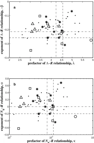
For the special case of exponential raindrop size distributions with a constant N₀, Eqns. (23) and (24) resolve the issue of relating the coefficients of power law Z–R relationships to the parameters of the raindrop size distribution. Generalizations of these expressions that allow one to cope with the case of a variable N₀ are derived in Appendix A. These expressions provide the opportunity to investigate the dependence of the parameters of the (exponential) raindrop size distribution on the type of rainfall. To this end, the coefficients of the 69 power law Z–R relationships quoted by Battan (1973) that have been discussed earlier, are used to invert Eqns. (23) and (24) and their generalizations presented in Appendix A (Eqns. (A7) and (A8) for the exponents of power law Z–R relationships, and Eqns. (A13) and (A14) for their prefactors). As demonstrated in Appendix A, this leads to power law Λ–R and N0–R

relationships for each of Battan’s Z–R relationships. Figure 3a presents the results for the coefficients of the corresponding Λ–R relationships (parameterised as

β

λ −

=

Λ R with Λ expressed in mm-1 _{and R in mm h}-1_{), Fig.}

3b for the coefficients of the corresponding N₀–R relationships (N₀ = κRα _{with N}

0 in mm-1 m-3 and R in mm h -1_{). Figure 3b clearly demonstrates that the assumption of a}

constant N₀ is too restrictive in practice. Although the mean value of α seems to be close to zero (indicating a constant

N₀ ), there is a significant amount of variability between different rainfall climatologies.

Although it is again difficult to associate unambiguously the coefficients of these power law relationships with particular rainfall types, it seems possible to distinguish some general tendencies. Both in terms of the Λ–R relationship

and in terms of the N₀ –R relationship, orographic rainfall tends to be associated with larger prefactors and smaller exponents. For thunderstorm rainfall, the opposite seems to be the case. Recall that Λ is the inverse of the mean diameter of raindrops present in a volume of air and that N₀ represents the concentration of the smallest raindrops (Eqn. (9)). Bearing this in mind, the observations indicate that, at a given rain rate, orographic rainfall would exhibit smaller mean raindrop sizes and larger concentrations, whereas thunderstorm rainfall would be associated with larger mean

2 2.5 3 3.5 4 4.5 5 5.5 6 −0.4 −0.3 −0.2 −0.1 0 a prefactor of Λ−R relationship, λ exponent of Λ − R relationship, − β 103 104 105 −0.8 −0.6 −0.4 −0.2 0 0.2 0.4 0.6 0.8 b prefactor of N 0−R relationship, κ exponent of N 0 − R relationship, α

Fig. 3. The coefficients λ and –β of power law Λ–R relationships Λ

= λR–β _{(with Λ expressed in mm}−1 _{and R in mm h}–1_{) for the 69}

exponential raindrop size distributions consistent with Battan’s (1973) Z–R relationships, stratified according to rainfall type: orographic (circles), thunderstorm (traingles), widespread/ stratiform (stars), showers (squares), no unambiguous identification possible (dots). The dashed line corresponds to the relationship Λ =

4.55R–0.258_{, consistent with Z = 200R}1.6 _{(Marshall et al., 1955); the}

dash-dotted line corresponds to the relationship Λ = 4.23R–0.214_,

consistent with Z = 237R1.50 _{(Marshall and Palmer, 1948).}

(b) Idem for the coefficients κ and α of the 69 corresponding power

law N₀–R relationships N₀ = κRα _{(with N}

0 expressed in mm–1 m–3 and

R in mm h–1_{). The dashed line corresondpons the relationship N}

0 =

1.13×104 _R–0.203_{, consistent with Z = 200R}1.6 _{(Marshall et al., 1955);}

the dash-dotted line corresponds to the relationship N₀ = 8.00×103_,

drop sizes and smaller concentrations. This is exactly what one would expect for these types of rainfall. Moreover, it provides an explanation for the differences between the coefficients of the Z–R relationships corresponding to these rainfall types. Although it seems difficult to derive similar interpretations for the other rainfall types from Fig. 3, the results demonstrate the usefulness of Eqns. (23) and (24) and their generalizations, Eqns. (A7, A8) and (A13, A14). CONSISTENT POWER LAW RADAR REFLECTIVITY– RAIN RATE RELATIONSHIPS

On the basis of the encountered ν(D),N0–R, Λ–R, and Z–R

power law relationships, i.e. ν(D) = 3.778D0.67 _{(Atlas and}

Ulbrich, 1977), N₀ = 8.0×103 _mm-1 _m-3_{, Λ − 4.1R}–0.21 _mm-1

(Marshall and Palmer, 1948), and Z = 200R1.6 _{(Marshall et} al., 1955), respectively, a total of six different consistent

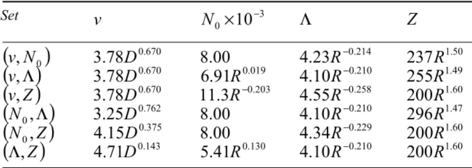
sets of power law relationships between rainfall-related variables can be constructed. This is because, as has been demonstrated earlier, each combination of two power law relationships selected from these four will imply the other two. Of the four variables v, N₀, Λ, and Z, six different combinations of two variables can be selected. Each of these pairs corresponds to a different (consistent) set of power law relationships.

Table 1 gives the power law v(D), N₀–R, Λ–R, and Z–R relationships for these six sets. The sets with a constant N₀ have already been encountered. For the other three sets, it is necessary to drop Marshall and Palmer’s (1948) restrictive assumption of a constant N₀. In those cases, N₀ becomes a power of the rain rate, too. The possibility of such power law N₀–R relationships has been suggested several times in the literature (e.g. Sekhon and Srivastava, 1971; Delrieu et

al., 1991; Sempere Torres et al., 1998). It has been

demonstrated already that the majority of Battan’s Z–R relationships also leads to exponential parameterisations

with variable N₀.

It is difficult to make general statements about differences in quality between these six sets of relationships. The reliability of a particular set depends on the plausibility of the corresponding parameterisation for the raindrop size distribution (Uijlenhoet and Stricker, 1999). It seems that the sets that are consistent with the raindrop terminal fall speed parameterisation of Atlas and Ulbrich (1977), i.e. the sets denoted (v, N₀), (v, Λ), and (v, Z), should be given a preference, as they seem to be most physically realistic. Figure 4 shows the Z–R relationships corresponding to these three sets, together with the envelope of Battan’s Z–R relationships (Fig. 1a,b). There seems to be little difference between these relationships, particularly for rain rates

Table 1. Six different consistent sets of power law relationships between

rainfall-related variables and the rain rate R (mm h-1_{) for exponential raindrop size}

distributions of the form N_v(D) = N₀ exp(–ΛD) mm-1 _m-3_{. Each set corresponds to}

a particular pair selected from the variables v (m s-1_{), N}

0 (mm-1 m-3), Λ (mm-1),

and Z (mm6 _m-3_{) (Uijlenhoet and Stricker, 1999).}

Set

_v

3 0

×

10

−

N

Λ

Z

(

v

, N

0

)

670 . 0

78

.

3

D

8

.

00

₄

_.

₂₃

_R

−0.214

_237R

1.50

( )

v

,

Λ

₃

_.

₇₈

_D

0.670

₆

_.

₉₁

_R

0.019

₄

_.

₁₀

_R

−0.210

_255R

1.49

( )

v,

Z

₃

_.

₇₈

_D

0.670

₁₁

_.

₃

_R

−0.203

₄

_.

₅₅

_R

−0.258

_200R

1.60

(

N

₀

,

Λ

)

₃

_.

₂₅

_D

0.762

₈

_.

₀₀

₄

_.

₁₀

_R

−0.210

_296R

1.47

(

N ,

₀

Z

)

₄

_.

₁₅

_D

0.375

₈

_.

₀₀

₄

_.

₃₄

_R

−0.229

_200R

1.60

(

Λ

,

Z

)

₄

_.

₇₁

_D

0.143

₅

_.

₄₁

_R

0.130

₄

_.

₁₀

_R

−0.210

_200R

1.60

Fig. 4. Comparison of three power law Z–R relationships that are

consistent with an exponential raindrop size distribution and Atlas and Ulbrich’s (1977) power law raindrop terminal fall speed parameterisation ν(D) = 3.778D0.67 _{m s}-1 _{(with D in mm): Z =}

237R1.50 _{(solid line), consistent with N}

0 = 8.00×103 mm-1 m-3 and Λ

= 4.23R–0.214 _mm-1_{;Z = 255R}1.49 _{(dashed line), consistent with N}

0 =

6.91×103 _R0.019 _mm-1 _m-3 _{and Λ = 4.10R}–0.210 _mm-1_{; Z = 200R}1.60

(dash-dotted line), consistent with N₀ = 1.13×104 _R–0.203 _mm-1 _m-3

and Λ = 4.55R–0.258 _mm-1_. 10 15 20 25 30 35 40 45 50 55 60 10−1 100 101 102

radar reflectivity factor, 10log(Z) (dBZ)

rain rate,

R

(mm h

−1

between 1 and 50 mm h-1_{, demonstrating that all three will}

provide reasonable representations of Z–R relationships for mean climatological conditions.

Summary and conclusions

Using the classical exponential raindrop size distribution introduced by Marshall and Palmer (1948) as an example, it has been demonstrated how the definitions of the radar reflectivity factor Z and the rain rate R in terms of that raindrop size distribution naturally lead to the ubiquitous power law Z–R relationships. It has also been demonstrated that Z is more naturally defined in terms of the size distribution of raindrops present in a volume of air, whereas

R is more naturally defined in terms of the size distribution

of raindrops arriving at a surface. Using these definitions, explicit expressions for the coefficients of power law Z–R relationships in terms of the parameters of the (exponential) raindrop size distribution have been derived.

These expressions have been used to analyse the 69 empirical Z–R relationships quoted by Battan (1973). The objective was to verify whether there exists any systematic difference in the coefficients of Z–R relationships and the corresponding parameters of the (exponential) raindrop size distribution between different rainfall types. It was found that, at a given rain rate, orographic rainfall tends to exhibit smaller mean raindrop sizes and larger concentrations, whereas thunderstorm rainfall tends to be associated with larger mean raindrop sizes and smaller concentrations, which is exactly what one would expect for these types of rainfall. This interpretation provides an explanation for the smaller values of the prefactors and the larger values of the exponents of the Z–R relationships reported for orographic rainfall as compared to those reported for thunderstorm rainfall. For the other rainfall types considered (widespread/ stratiform and showers), it was difficult to obtain unambiguous interpretations of the coefficients of the corresponding Z–R relationships.

Finally, six consistent Z–R relationships have been derived, based upon different assumptions regarding the rain rate dependence of the parameters of the (exponential) raindrop size distribution. There seemed to be little difference between the three relationships that were considered to be the most physically realistic, showing that all three would provide reasonable representations of Z–R relationships for mean climatological conditions. Appendix A shows that the six relationships are in fact special cases of a general Z–R relationship that follows from a recently proposed scaling framework for describing raindrop size distributions and their properties.

References

Andrieu, H. and Creutin, J.-D., 1995. Identification of vertical profiles of radar reflectivity for hydrological applications using an inverse method. 1. Formulation. J. Appl. Meteorol., 34, 225– 239.

Andrieu, H., Delrieu, G. and Creutin, J.-D., 1995. Identification of vertical profiles of radar reflectivity for hydrological applications using an inverse method. 2. Sensitivity analysis and case-study. J. Appl. Meteorol., 34, 240–259.

Andrieu, H., Creutin, J.-D., Delrieu, G. and Faure, D., 1997. Use of a weather radar for the hydrology of a mountainous area. Part I: radar measurement interpretation. J. Hydrol., 193, 1–25. Atlas, D. and Ulbrich, C.W., 1977. Path- and area-integrated rainfall measurement by microwave attenuation in the 1-3 cm band. J. Appl. Meteorol., 16, 1322–1331.

Atlas, D., Srivastava, R.C. and Sekhon, R.S., 1973. Doppler radar characteristics of precipitation at vertical incidence. Rev.

Geophys. Space Phys., 11, 1–35.

Battan, L.J., 1973. Radar observation of the atmosphere. The University of Chicago Press, Chicago, 324 pp.

Bennett, J.A., Fang, D.J. and Boston, R.C., 1984. The relationship between N₀ and λ for Marshall-Palmer type raindrop-size distributions. J. Clim. Appl. Meteorol., 23, 768–771.

Cluckie, I.D., Griffith, R.J., Lane, A. and Tilford, K.A., 2000. Radar hydrometeorology using a vertically pointing radar.

Hydrol. Earth Syst. Sci., 4, 565–580.

Collier, C.G., 1989. Applications of weather radar systems: a guide

to uses of radar data in meteorology and hydrology. Ellis

Horwood, Chichester, UK. 294 pp.

Collier, C.G., 1993. The application of a continental-scale radar database to hydrological process parametrization within Atmospheric General Circulation Models. J. Hydrol., 142, 301– 318.

Creutin, J.-D., Andrieu, H. and Faure, D., 1997. Use of a weather radar for the hydrology of a mountainous area. Part II: radar measurement validation. J. Hydrol., 193, 26–44.

Delrieu, G., Creutin, J.-D. and Saint André, I., 1991. Mean K–R relationships: practical results for typical weather radar wavelengths. J. Atmos. Ocean. Technol., 8, 467–476. Feingold, G. and Levin, Z., 1986. The lognormal fit to raindrop

spectra from convective clouds in Israel. J. Clim. Appl.

Meteorol., 25, 1346–1363.

Gunn, R. and Kinzer, G.D., 1949. The terminal velocity of fall for water droplets in stagnant air. J. Meteorol., 6, 243–248. Hall, R.L. and Calder, I.R., 1993. Drop size modification by forest

canopies: measurements using a disdrometer. J. Geophys. Res.

(D), 98, 18465–18470.

Illingworth, A.J., Blackman, T.M. and Goddard, J.W.F., 2000. Improved rainfall estimates in convective storms using polarisation diversity radar. Hydrol. Earth Syst. Sci., 4, 555– 563.

Joss, J. and Gori, E.G., 1978. Shapes of raindrop size distributions.

J. Appl. Meteorol., 17, 1054–1061.

List, R., 1988. A linear radar reflectivity – rain rate relationship for steady tropical rain. J. Atmos. Sci., 45, 3564–3572. Marshall, J.S. and Palmer, W.M., 1948. The distribution of

raindrops with size. J. Meteorol., 5, 165-166.

Marshall, J.S., Hitschfeld, W. and Gunn, K.L.S., 1955. Advances in radar weather. Adv. Geophys., 2, 1–56.

Sanchez Diezma, R., Zawadzki, I. and Sempere Torres, D., 2000. Identification of the bright band through the analysis of volumetric radar data. J. Geophys. Res. (D), 105, 2225–2236. Sekhon, R.S. and Srivastava, R.C., 1971. Doppler radar

observations of drop-size distributions in a thunderstorm. J.

Sempere Torres, D., Porrà, J.M. and Creutin, J.-D., 1994. A general formulation for raindrop size distribution. J. Appl. Meteorol., 33, 1494–1502.

Sempere Torres, D., Porrà, J.M. and Creutin, J.-D., 1998. Experimental evidence of a general description for raindrop size distribution properties. J. Geophys. Res. (D), 103, 1785–1797. Smith, J.A., 1993. Marked point process models of raindrop-size

distributions. J. Appl. Meteorol., 32, 284–296.

Smith, J.A. and Krajewski, W.F., 1993. A modeling study of rainfall rate – reflectivity relationships. Water Resour. Res., 29, 2505–2514.

Uijlenhoet, R., 1999. Parameterisation of rainfall microstructure

for radar meteorology and hydrology. Doctoral dissertation,

Wageningen University, The Netherlands, 279 pp.

Uijlenhoet, R. and Stricker, J.N.M., 1999. A consistent rainfall parameterisation based on the exponential raindrop size distribution. J. Hydrol., 218, 101–127.

Ulbrich, C.W., 1983. Natural variations in the analytical form of the raindrop size distribution. J. Clim. Appl. Meteorol., 22, 1764–1775.

Ulbrich, C.W., 1985. The effects of drop size distribution truncation on rainfall integral parameters and empirical relations.

J. Clim. Appl. Meteorol., 24, 580–590.

Ulbrich, C.W. and Atlas, D., 1998. Rainfall microphysics and radar properties: analysis methods for raindrop size spectra. J. Appl.

Meteorol., 37, 912–923.

Wood, S.J., Jones, D.A. and Moore, R.J., 2000. Accuracy of rainfall measurement for scales of hydrological interest. Hydrol.

Earth Syst. Sci., 4, 531–541.

Zawadzki, I., 1984. Factors affecting the precision of radar measurements of rain. Preprints of the 22nd _{Conference on Radar}

Meteorology, 251-256. American Meteorological Society,

Boston.

Appendix A

A general framework for radar

reflectivity–rain rate relationships

Sempere Torres et al. (1994, 1998) have recently demonstrated that all previously proposed parameterisations for the raindrop size distribution are special cases of a general formulation, which takes the form of a scaling law. In this formulation, the raindrop size distribution depends both on the raindrop diameter (D) and on the value of a so-called reference variable, commonly taken to be the rain rate (R). The generality of this formulation stems from the fact that it is no longer necessary to impose an a priori functional form for the raindrop size distribution. Moreover, it naturally leads to the ubiquitous power law relationships between rainfall integral parameters, notably that between the radar reflectivity factor (Z) and R.

According to the scaling law formalism, raindrop size distributions can be parameterized as (Sempere Torres et

al., 1994, 1998)

)

/

(

)

,

(

_D

_R

_R

α

_g

_D

_R

β

N

V

=

, (A1)

where N_V (D, R) (mm-1 _m-3_{) is the raindrop size distribution}

as a function of the (equivalent spherical) raindrop diameter

D (mm) and the rain rate R (mm h-1_{), α and β are}

(dimensionless) scaling exponents, and g(x) is the general

raindrop size distribution as a function of the scaled raindrop

diameter x = D / Rβ _{. In agreement with common practice, R}

is used as the reference variable in Eqn. (A1), although any other rainfall integral variable could serve as such (notably

Z). According to this formulation, the values of α and β and the form and dimensions of g(x) depend on the choice of the reference variable, but do not bear any functional dependence on its value.

The importance of the scaling law formalism for radar hydrology stems from the fact that it allows an interpretation of the coefficients of Z–R relationships in terms of the values of the scaling exponents and the shape of the general raindrop size distribution. Substituting Eqn. (A1) into the definition of Z in terms of the raindrop size distribution (Eqn. (2) leads to the power law

b aR Z = , (A2) with

∫

∞ = 0 6_{g( dxx)} x a _{, (A3)} and β α 7+ = b (A4)

(Uijlenhoet, 1999). Hence, the prefactors of power law Z–

R relationships are entirely determined by the shape of the

general raindrop size distribution (they are in fact its 6th moment), whereas a linear combination of the values of the scaling exponents completely determines the exponents of such power law Z–R relationships.

In a similar manner, the scaling law formalism leads to power law relationships between any other pair of rainfall integral variables. In particular, substituting Eqn. (A1) into the definition of R in terms of the raindrop size distribution and a power law raindrop terminal fall speed parameterisation (Eqns. (4) and (5)) leads to the

self-consistency constraints 1 ) ( 10 6 0 3 4 ₌ × − _c∞

_∫

_x +γ_{g x dx} π (A5) and

(

4₊

)

₌1 + γ β α (A6)

(Sempere Torres et al., 1994). Hence, g(x) must satisfy an integral equation (which reduces its degrees of freedom by one) and there is only one free scaling exponent. Substitution of the self-consistency constraint on the scaling exponents (Eqn. (A6)) into the definition of b in terms of those scaling exponents (Eqn. (A4)) yields

α γ γ γ + − − + = 4 3 4 7 b (A7)

in terms of the scaling exponent α, or equivalently

(

−γ

)

β

+ =1 3

b (A8)

in terms of the scaling exponent β (Uijlenhoet, 1999). For γ = 0.67 (Atlas and Ulbrich, 1977), Eqn. (A7) reduces to

b = 1.50 – 0.50α and Eqn. (A8) to b = 1 + 2.33β. Hence, the exponents of power law Z–R relationships can be expressed explicitly in terms of both scaling exponents (which are related to each other via the self-consistency constraint Eqn. (A6)), independent of any assumption regarding the shape of the general raindrop size distribution. To obtain equivalent explicit expressions for the prefactors of power law Z–R relationships, however, a particular functional form for g(x) needs to be assumed.

As an example, appropriate for the purpose of this paper, consider an exponential parameterisation for the general raindrop size distribution,

( )

x

exp

(

x

)

.

g

=

κ

−

λ

(A9)

In this general form, g(x) is not an admissible description of the general raindrop size distribution, because it does not satisfy the self-consistency constraint on g(x) (Eqn. (A5)). Substitution of Eqn. (A9) into (A5) yields a power law relationship of κ in terms of λ,

(

)

[

6_π 10 4 4 _γ

]

1_λ4 γ,

κ _{= ×} − _{cΓ +} − + (A10)

or equivalently, a power law relationship of λin terms of κ,

(

)

[

]

( ) _{( )} . 4 10 6_π 4 _γ 1/4γ _κ1/4γ λ_{= ×} − _{cΓ +} + + (A11)

Eqns. (A10) and (A11) provide explicit forms of the self-consistency constraint on g(x) for the special case of an exponential parameterisation. For the applied units, with

c = 3.778 and γ = 0.67 (Atlas and Ulbrich, 1977), Eqn. (A10) reduces to κ = 9.50λ4.67 _{and Eqn. (A11) to λ =}

0.618κ0.214_.

Hence, the self-consistency constraint on g(x) reduces its number of free parameters by one. Since the exponential parameterisation for g(x) only has two parameters, namely

κ and λ (Eqn. (A9)), the number of free parameters that remains, is only one (either κ or λ). In the same way as Eqn. (A6) describes a unique relationship between the scaling exponents α and β (depending only on the value of γ), Eqns. (A10) and (A11) describe a unique relationship between the parameters of the exponential form for the general raindrop size distribution (depending only on the values of

c and γ). As a result, for the special case of an exponential parameterisation for g(x), the total number of free parameters that is required to describe unambiguously the scaling law (Eqn. (A1)) and any derived (power law) relationship between rainfall-related variables (notably Z–R relationships) is two: on the one hand either α or β, and on the other hand either κ or λ (Sempere Torres et al., 1994, 1998). Note that relationships similar to Eqns. (A10) and (A11) could be developed for any other functional form for the general raindrop size distribution (notably the gamma and log-normal parameterisations), but such an exercise would be beyond the scope of this paper (Uijlenhoet, 1999). A general expression for the prefactors of power law Z–R relationships for the special case of an exponential parameterisation for g(x) can be obtained by substituting Eqn. (A9) into (A3). This yields

( )

7 −7. Γ

= κλ

a (A12)

To guarantee that a satisfies the self-consistency constraint on g(x), either Eqn. (A10) or (A11) needs to be substituted into Eqn. (A12). The latter yields a power law relationship of a in terms of κ,

( )

₇

[

_6π×10−4 _Γ

(

_4+γ

)

]

−7/(4+γ)_κ−( ) (3−γ/4+γ)_,

Γ

= c

a (A13)

the former an equivalent power law relationship of a in terms of λ,

` a=Γ

( )

7

[

6π×10−4cΓ

(

4+γ

)

]

−1λ−( )3−γ. (A14)

These equations complement Eqns. (A7) and (A8) and together form an internally consistent set of relationships for the estimation of the prefactors and exponents of power law Z–R relationships in terms of the parameters of the exponential raindrop size distribution. For the applied units, with c = 3.778 and g = 0.67 (Atlas and Ulbrich, 1977), Eqn. (A13) reduces to a = 2.10×104_k–0.50 _{and Eqn. (A14) to} a = 6.84×103 _l–2.33_.

Equations (A13) and (A14) can also be inverted to estimate λ and κ from given values of a, in much the same way as Eqns. (A7) and (A8) can be inverted to estimate α and β from given values of b. This method has been applied in Fig. 3, where the 69 power law Z–R relationships quoted

by Battan (1973) have been employed to infer values of the parameters α, β, κ and λ for different types of rainfall.

It is of considerable interest to establish a link between the scaling law formalism and the traditional analytical parameterisations for the raindrop size distribution. For the special case of the exponential raindrop size distribution, this can be achieved through substituting Eqn. (A9) into (A1). This yields

(

D,R

)

R exp

(

R D

)

.

N_{V =κ} α _−λ −β (A15)

A comparison with Eqn. (9) shows that Eqn. (A15) reduces to the classical exponential parameterisation for the raindrop size distribution if N₀ and Λ depend on R according to the power laws α κR N0= (A16) and . β λ − = Λ R (A17)

It is important to recognize that Eqn. (A15) differs from Eqn. (9) in two fundamental ways:

(1) As opposed to Eqn. (9), the scaling law (Eqn. (A1)) and its particular functional form for the special case of an exponential parameterisation for g(x) (Eqn. (A15))

explicitly consider the functional dependence of the

raindrop size distribution on the reference variable R, not just on the raindrop diameter D. As a result, the scaling law formalism clarifies the way in which N₀ and Λ should be interpreted: not as parameters, as the functional form of Eqn. (9) seems to suggest, but as (rainfall-related) variables that exhibit an explicit dependence on the reference variable R. The parameters of the exponential parameterisation for the raindrop size distribution are not N₀ and Λ, but α, β, κ and λ (Eqn. (A15));

(2) As opposed to Eqn. (9), Eqn. (A15) is an intrinsically self-consistent form of the exponential raindrop size distribution. This is because, as has been demonstrated above, only two of the four parameters (α, β, κ, λ) that define N_V (D,R) according to Eqn. (15) can actually be

chosen freely. More concretely, the coefficients of the power law N₀–R and Λ–R relationships defined by Eqns. (A16) and (A17) cannot be chosen without restrictions, but have to satisfy the self-consistency constraints imposed by Eqns. (A6) and (A10) (or (A11)).

Finally, consider Marshall and Palmer’s (1948) restrictive assumption of a constant N₀, independent of the rain rate R. Equation (A16) shows that this special case corresponds to

N₀ =κ, or equivalently α = 0. Substitution of N₀ =κ in Eqn. (A13) yields an equation that is identical to the expression for a derived in the main text (Eqn. (23)). Substitution of α = 0 in Eqn. (A7) gives b = 7/(4 + γ) , identical to Eqn. (24). In a similar manner, substituting N₀ =κ and α = 0 in Eqns. (A11) and (A6), respectively, leads to a power law Λ–R relationship (Eqn. (A17)) with coefficients identical to those of the relationship derived in Eqn. (19). Hence, the equations derived here are consistent generalizations of Eqns. (19– 24), valid for the general exponential case where N₀ bears a power law dependence on R. They reduce to Eqns. (19) and (22)–(24) for the special case of a constant N₀.

Acknowledgements

The author is indebted to Han Stricker (Wageningen University and Research Centre, Department of Environmental Sciences, Sub-department Water Resources), Josep M. Porrà (formerly at Universitat de Barcelona, Departament de Física Fonamental), and Daniel Sempere Torres (Universitat Politècnica de Catalunya, Departament d’Enginyeria Hidràulica, Marítima i Ambiental) for providing useful suggestions to improve the manuscript. Financial support for this research has been provided by the Commission of the European Communities under the EPOCH and ENVIRONMENT programmes (Contracts No. EPOC–CT90–0026, EV5V–CT92–0182 and ENV4–CT96– 5030).