Dynamic Trading and Behavioral Finance
by
Alexander Remorov
Submitted to the Sloan School of Management
in partial fulfillment of the requirements for the degree of
Doctor of Philosophy in Operations Research
at the
MASSACHUSETTS INSTITUTE OF TECHNOLOGY
June 2016
c
○
Massachusetts Institute of Technology 2016. All rights reserved.
Author . . . .
Sloan School of Management
April 26, 2016
Certified by . . . .
Andrew W. Lo
Charles E. and Susan T. Harris Professor
Director of Laboratory for Financial Engineering
Thesis Supervisor
Accepted by . . . .
Dimitris Bertsimas
Boeing Leaders for Global Operations Professor
Co-Director, Operations Research Center
Dynamic Trading and Behavioral Finance
by
Alexander Remorov
Submitted to the Sloan School of Management on April 26, 2016, in partial fulfillment of the
requirements for the degree of
Doctor of Philosophy in Operations Research
Abstract
The problem of investing over time remains an important open question, considering the recent large moves in the markets, such as the Financial Crisis of 2008, the subsequent rally in equities, and the decline in commodities over the past two years. We study this problem from three aspects.
The first aspect lies in analyzing a particular dynamic strategy, called the stop-loss strat-egy. We derive closed-form expressions for the strategy returns while accounting for serial correlation and transactions costs. When applied to a large sample of individual U.S. stocks, we show that tight stop-loss strategies tend to underperform the buy-and-hold policy due to excessive trading costs. Outperformance is possible for stocks with sufficiently high serial correlation in returns. Certain strategies succeed at reducing down-side risk, but not substantially. We also look at optimizing the stop-loss level for a class of these strategies.
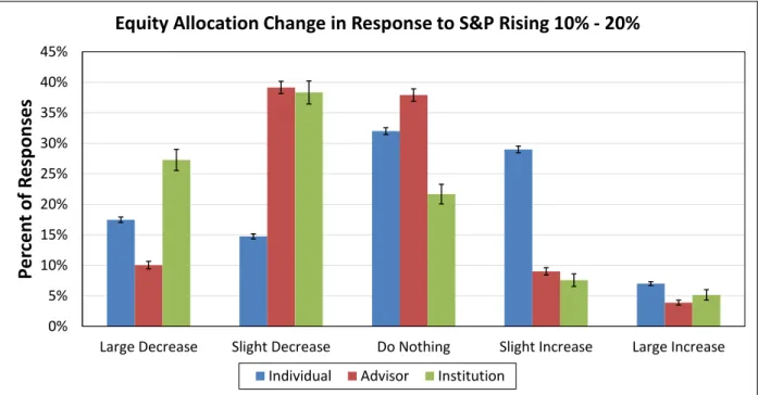
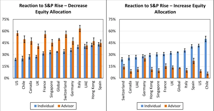
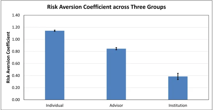
The second approach is more behavioral in nature and aims to elicit how various mar-ket players expect to react to large changes in asset prices. We use a global survey of individual investors, financial advisors, and institutional investors to do this. We find that most institutional investors expect to exhibit highly contrarian reactions to past re-turns in terms of their equity allocations. Financial advisors are also mostly contrarian; a few of them demonstrate passive behavior. In contrast, individual investors are, on average, extrapolative, and can be partitioned into four distinct types: passive investors, risk avoiders, extrapolators, and everyone else.
The third part of the thesis studies how people actually trade. We propose a new model of dynamic trading in which an investor is affected by behavioral heuristics, and carry out extensive simulations to understand how the heuristics affect portfolio performance. We propose an MCMC algorithm that is reasonably successful at estimating model pa-rameters from simulated data, and look at the predictive ability of the model. We also provide preliminary results from looking at trading data obtained from a brokerage firm. We focus on understanding how people trade their portfolios conditional on past returns at various horizons, as well as on past trading behavior.
Thesis Supervisor: Andrew W. Lo
Acknowledgments
I would like to thank my advisor, professor Andrew Lo, for his continuous guidance, support, and motivation throughout my thesis. I am very grateful to have been working with him on very interesting and exciting projects that I truly enjoyed. Andrew’s brilliant intuition and big picture thinking, wealth of knowledge and new ideas, and amazing work ethic made it a great honor and pleasure to work with him and learn from him. His advice and thoughts on various aspects of academia, industry and life in general have been and definitely will be extremely helpful for me throughout my entire career.
I am very grateful for continuous research discussion and guidance with my other committee members: professors Dimitris Bertsimas, Leonid Kogan, and Hui Chen. I learned a lot about the power of analytics and optimization from the classes I took with Dimitris and conversations I had with him. Leonid and Hui were extremely helpful in teaching me and providing advice on how to build and extend financial models, especially from an asset pricing perspective in which they are truly experts.
It was great to work with Daniel Elkind during the last few months of my degree. The project on modeling investor trading really took off after he came on board, and we have been able to produce great results at a very fast pace due to his great enthusiasm and hard work, as well as very productive discussion. I wish him all the best during the remainder of his Ph.D. and I am sure he will do great.
The research collaboration that Andrew and I had with Natixis Asset Management was crucial for producing the results of this thesis. David Goodsell and Stephanie Gi-ardina did a great job in designing and carrying out investor surveys; it was also very helpful to continuously discuss the progress and the results with them. Support from John Hailer is also very much appreciated.
I also want to acknowledge the terrific help of the U.S. retail brokerage firm that provided us with the trading data towards the end of my thesis. The individuals at the firm responsible for delivering the data were extremely responsive and involved in compiling and sending the data and ensuring it is clean and satisfies our joint research purposes. Even though only preliminary results of this joint project are included in this thesis, I am truly excited about this project and hope that it will produce some amazing results down the road.
helpful with the many questions I had throughout my time here and took care of any relevant administrative items in a very timely and helpful manner. I also want to thank Andrew’s secretaries Jayna Cummings, Patsy Thompson, and Allison McDonough for being very responsive and always being able to fit me into Andrew’s busy schedule.
My Ph.D. would not be the same without all the great people I met here. Charles T., Velibor M., Andrew L., Will M., Shalev B., Anna P., Stefano T., Alexandre S., Daniel S., Ali A., Alex W., Virgile G., Joey H., Zach O., Arthur F., Adam E., David F., Ludovica R., Mariapola T., and Dan S. are some of the awesome students that made the last four years such a fun and fulfilling experience. It was also an awesome experience leading the ORC soccer team, and I want to thank my fellow teammates Nikita, Anurag, Kevin, Marnix, Adam, Osman, Fransisco, Elliott, Joey, Virgile, Max, Hai, Alex S., Alex W., David, Will, and Charles, among others for coming to the pick-up and intramurals games and playing the great game together. I have a lot of fond memories from the two years I lived with my two roommates and very close friends Danny Shi and David Rush, especially when we played Settlers (and particularly the games which I won).
I want to thank Edwin Cao for being an amazing friend. We had a lot of entertaining conversations and heated discussions on all kinds of topics ranging from analytics to Texas to nuggets, and I truly cherish the fact that we were able to talk almost every day besides often being in different cities or even countries. Edwin’s continuous grind to be tier 1 or nothing will always continue to be a great source of motivation for me.
I want to thank my family for their continuous encouragement and support throughout my thesis and also throughout my whole life. Particularly my mother and father, who have taught me so much and have always done their best for me. I would not be here without them.
Finally, I want to thank my wife Kristina for all her care and love. For being so understanding and supportive. For being a constant source of inspiration and happiness. For always being by my side. I love you.
Contents
1 Stop-loss Strategies with Serial Correlation, Regime Switching and
Trans-action Costs 1
1.1 Introduction . . . 2
1.2 Literature review . . . 4
1.3 Analytical results . . . 6
1.3.1 Strategy returns for an AR(1) process . . . 7
1.3.2 Impact of trading costs . . . 9
1.4 Simulation analysis . . . 10
1.4.1 AR(1) process . . . 11
1.4.2 Regime-switching process . . . 12
1.5 Empirical analysis . . . 16
1.5.1 Data and methodology . . . 19
1.5.2 Strategy performance . . . 20
1.5.3 Delayed stop-loss strategies . . . 26
1.6 Optimizing Stop-Loss Level . . . 27
1.6.1 Applying SDP to Stop-Loss Problem . . . 30
1.6.2 Optimization Results . . . 32
1.7 Conclusion . . . 36
1.8 Appendix . . . 39
1.8.1 Proof of Proposition 1 . . . 39
1.8.2 Proof of Proposition 2 . . . 43
1.8.3 Definition of Delayed Stop-Loss Strategy . . . 44
1.8.4 Discussion of strategy returns regression results . . . 44
1.8.6 Supplemental tables and figures . . . 48
1.8.7 Historical strategy performance and regime-switching . . . 51
1.8.8 Volatility-adjusting stop-loss strategies . . . 55
2 Measuring Risk Preferences and Asset-Allocation Decisions: A Global Survey Analysis 58 2.1 Introduction . . . 59
2.2 Methodology . . . 61
2.3 Investors, Advisors, and Institutions . . . 65
2.4 Individual Investor Decisions . . . 71
2.5 Individual Investor Predictive Analytics . . . 78
2.6 Conclusion . . . 81
2.7 Appendix . . . 85
2.7.1 Individual Investor and Institutional Survey Questions . . . 85
2.7.2 Financial Advisor Survey Questions . . . 86
2.7.3 Survey Respondents Characteristics . . . 87
3 Algorithmic Models of Investor Behavior 93 3.1 Introduction . . . 94
3.2 Decision-Making Framework . . . 96
3.2.1 The Disposition Effect . . . 97
3.2.2 Loss Aversion . . . 99
3.2.3 Overconfidence . . . 100
3.2.4 The Gambler’s and Hot Hand Fallacies . . . 101
3.2.5 Regret . . . 103
3.2.6 Anchoring . . . 104
3.3 Model Parameters . . . 105
3.3.1 Default Strategy and Heuristic Weights . . . 106
3.3.2 Heuristic Parameters . . . 107
3.4 Simulation Analysis . . . 109
3.5.1 Empirical Results for Pairs of Heuristics . . . 119
3.5.2 Empirical Heuristic Correlations . . . 122
3.6 Model Inference . . . 125 3.6.1 Modeling Framework . . . 125 3.6.2 MCMC Estimation . . . 127 3.6.3 Single Investor . . . 128 3.6.4 Multiple Investors . . . 133 3.7 Predictive Analytics . . . 146
3.7.1 The Prediction Problem . . . 146
3.7.2 Performance Measures . . . 147
3.7.3 Predictive Accuracy of Single and Pairwise Heuristics . . . 148
3.7.4 Predictive Accuracy for All Heuristics . . . 149
3.8 Conclusion . . . 151
3.9 Appendix . . . 156
4 Preliminary Analysis of Trading Data 165 4.1 Introduction . . . 165
4.2 Data Description . . . 167
4.3 Trading Distribution Analysis Methodology . . . 169
4.3.1 Computing Past Returns . . . 169
4.3.2 Computing Net Trade . . . 171
4.3.3 Computing Trading Indicator . . . 173
4.3.4 Computing Conditional Distributions . . . 173
4.4 Trading Distribution . . . 174
4.5 Dependence on Past History . . . 181
4.6 Conclusion and Next Steps . . . 191
4.7 Appendix . . . 192
Chapter 1
Stop-loss Strategies with Serial
Correlation, Regime Switching and
Transaction Costs
(joint work with Andrew W. Lo)
Abstract
Stop-loss strategies are commonly used by investors to reduce their holdings in risky assets if prices or total wealth breach certain pre-specified thresholds. We derive closed-form expressions for the impact of stop-loss strategies on asset returns that are serially correlated, regime switching, and subject to transaction costs. When applied to a large sample of individual U.S. stocks, we show that tight stop-loss strategies tend to under-perform the buy-and-hold policy in a mean-variance framework due to excessive trading costs. Outperformance is possible for stocks with sufficiently high serial correlation in returns. Certain strategies succeed at reducing downside risk, but not substantially. We also look at optimizing the stop-loss level for a class of these strategies.
Keywords: Stop-loss strategy; Risk management; Investments; Portfolio management; Asset allocation; Behavioral finance
1.1 Introduction
Many investors attempt to limit the downside risk of their investments by using stop-loss strategies, the most common of which is the stop-stop-loss order, a standing order to liquidate a position when a security’s price crosses a pre-specified threshold. By closing out the position, the investor is hoping to avoid further losses.
If prices follow random walks, any price movement in the past has no bearing on future returns—as long as the risky asset has a positive risk premium, the investor’s portfolio will have a higher expected return by staying invested in the asset rather than liquidating it after its price reaches a particular limit. In this case, Kaminski and Lo (2014) have shown that the stop-loss strategy tends to underperform a buy-and-hold strategy. However, there is extensive evidence that financial asset prices do not follow random walks (e.g., Lo and MacKinlay, 1988; Poterba and Summers, 1988; Jegadeesh and Titman, 1993). A natural question is whether these departures from randomness can be exploited using a dynamic investment strategy, including stop-loss policies.
In this paper, we focus on simple dynamic strategies incorporating stop-loss rules to determine how they compare to static buy-and-hold strategies. We provide closed-form expressions for the returns of a large class of these strategies and derive conditions under which they underperform or outperform buy-and-hold. Assuming that prices fol-low a first-order autoregressive process, we prove that the log-returns of “tight” stop-loss strategies—strategies with price triggers that are close to the asset’s current price— are approximately linear in the interaction term between autocorrelation and volatility, providing an explicit relation between the profitability of a stop-loss policy, return pre-dictability, and volatility. This expression yields bounds on how large return autocorrela-tion and volatility must be to beat a buy-and-hold strategy after accounting for trading costs.
We also consider the dynamic optimization problem of an investor trading a risky asset and a risk-free asset, with the returns of the risky asset following an AR(1) process. Consistent with our approximation results, optimal stop-loss behavior arises only when we have positive serial correlation in returns; furthermore, an investor should use a tighter stop-loss level for higher values of serial correlation and volatility of the process.
We extend our theoretical analysis by simulating various return processes and by com-paring the performance of stop-loss and buy-and-hold policies in a mean-variance
frame-work. We consider two general processes—an AR(1) and a regime-switching process—and vary the underlying parameters for each. In the first case, with a high enough serial cor-relation and volatility, the stop-loss strategy provides superior risk-adjusted returns in comparison to the buy-and-hold strategy. In the regime-switching case, the stop-loss strategy gives better performance in a few cases, and this outperformance comes from a large reduction in volatility rather than an improvement in raw returns. We also look at the tail performance of the strategy, as measured by skewness and maximum drawdown. We find that if a longer horizon for past returns is used to make the decision whether to stop out or not, downside risk tends to improve over the buy-and-hold.
To illustrate the practical relevance of stop-loss strategies, we perform a detailed empirical analysis of the performance of these strategies using a large sample of U.S. stock returns from 1964 to 2014. To derive realistic measures of performance, we incorporate transaction costs in our backtests by using bid-ask spreads, as well as historical estimates
when such spreads are missing.1 Our empirical findings are most relevant to short-term
traders, who usually employ tight stop-loss policies and frequently change their positions. We find that the performance of tight stop-loss strategies is closely related to the realized return autocorrelation over the investment period, which supports the common trading adage: “The trend is your friend." However, such strategies require a lot of trading, leading to high transaction costs. As a result, tight stop-loss strategies are able to outperform the buy-and-hold strategies only when asset returns are significantly serially correlated.
Of course, a stop-loss rule alone does not fully define an entire investment strategy since, after exiting a risky investment, the investor must decide when to re-enter. We consider several simple re-entry policies as part of our definition of a stop-loss rule and demonstrate that it is usually beneficial to re-invest soon after being stopped out in the case of tight stops. Another aspect that must be considered is where cash is invested after a stop-out. Assuming that cash is immediately invested in a risk-free asset, we show that the risk-free rate has a significant impact on the effectiveness of a stop-loss strategy, and this impact reconciles some of the inconsistencies among existing empirical studies of stop-loss strategies.
bias known as the “disposition effect” first documented by Shefrin and Statman (1985). The presence of behavioral biases such as this has been well documented in the finance
literature.2 While most of this research has focused on the empirical evidence for these
biases and the theoretical models to explain them, few studies have proposed methods for investors to actively avoid or protect against such biases. Stop-loss strategies are an important first step in this direction.
1.2 Literature review
Kaminski and Lo (2014) lay out the first general framework for analyzing stop-loss strategies. They start with analytical results for the performance of a stop-loss policy and consider three cases for the return process of the risky asset. For a simple random walk, the policy always produces lower expected returns. For an AR(1) process, the policy improves performance in the case of momentum, but hurts performance in the case of mean reversion. For a two-state Markov regime-switching model, the strategy sometimes gives better performance, since it tends to outperform the buy-and-hold strategy only in the low-mean state.
There are a few other analytical studies of stop-loss strategies. Glynn and Iglehart (1995) derive an optimal strategy by demonstrating that the expected value of the stock price at the time of exit satisfies a relatively simple ordinary differential equation (ODE). They also present an example of a utility function with a very heavy penalty on losses, which would lead the investor to set up a finite stop-loss limit. This contrasts with the case of constant relative risk aversion (CRRA) utility, where it is optimal to not use a stop-loss (Merton, 1969). Glynn and Iglehart’s ODE approach was later applied to derive the optimal selling rule in more complicated settings for the return distribution, including for a regime-switching process (Zhang, 2001; Pemy, 2011) and a mean-reverting process (Zhang and Zhang , 2008; Ekström, Lindberg, and Tysk, 2011). Besides the ODE approach, Abramov, Khan, and Khan (2008) analyze the trailing stop strategy in a discrete time framework, while Esipov and Vaysburd (1999) present a partial differential equation approach for analyzing stop-loss policies.
With respect to the empirical literature on stop-loss strategies, Kaminski and Lo
(2014) consider the strategy of investing in the S&P 500, using monthly frequency for the historical returns and U.S. long-term bonds as the “safe” asset. Erdestam and Stangenberg (2008) and Snorrason and Yusupov (2009) study the strategies applied to stocks in the OMX Stockholm 30 Index. Lei and Li (2009) use daily data for individual U.S. stocks (with the S&P 500 and the one-month U.S. T-bill considered as the “safe" assets) and conclude that traditional stop-loss strategies are able to reduce losses for some stocks, but not for others. Trailing stop-loss strategies are found to consistently reduce investment risk.
There has been little attention paid to the transaction costs associated with stop-loss strategies. Two papers that do address this issue are Macrae (2005) and Detko, Ma, and Morita (2008). They note that in many cases, the associated hidden costs, such as slippage, result in lower strategy returns.
Finally, stop-loss strategies may also benefit investors by implicitly correcting for some of their behavioral biases. One such bias is the disposition effect, where investors tend to hold losers for too long and sell winners too early, as documented by Shefrin and Statman (1985), Ferris, Haugen and Makhija (1988), and Odean (1998). Wong, Carducci, and White (2006) find evidence for the disposition effect in an experimental setting and propose using stop-loss orders to offset this bias. However, studies exploring this possibility have yielded mixed and inconclusive results. For example, Garvey and Murphy (2004) investigate a sample of trading records for professional traders in the U.S. and find that, while traders tend to use stop-loss orders and avoid large losses, they still exhibit the disposition effect. Nevertheless, Richards, Rutterford, and Fenton-O’Creevy (2011) find that retail investors who employ stop-loss strategies exhibit the disposition effect to a smaller extent than those who do not.
We build on the existing literature in several important directions. The first is an advanced theoretical formula approximating stop-loss strategy performance when returns follow an AR(1) process. We link the conclusions from this formula to historical stop-loss performance. The second direction is that we rigorously incorporate transaction costs into our analysis of simulated and historical strategy performance. The sample of assets we consider is individual U.S. stocks, which has different dynamics to the S&P 500 futures
Finally, we perform extensive simulations to gain insights on how the performance of the strategies is related to their specifications and the parameters of the underlying returns process.
1.3 Analytical results
We consider the stop-loss strategy introduced by Kaminski and Lo (2014) and later generalized by Erdestam and Stangenberg (2008). We invest 100% in the risky asset at the start of the period. If its cumulative return over 𝐽 consecutive periods drops below a specified threshold 𝛾, we liquidate our position and invest in the risk-free asset; otherwise we stay fully invested. To buy the asset again, the cumulative return over 𝐼 periods has to exceed a threshold 𝛿.
Denote by 𝑟𝑡 the log return on the risky asset at time 𝑡. Define the cumulative log
return 𝑅𝑡(𝑁 ) over 𝑁 consecutive periods as:
𝑅𝑡(𝑁 ) ≡
𝑁 ∑︁
𝑗=1
𝑟𝑡−𝑗+1 . (1)
Let 𝑠𝑡 be the proportion of wealth allocated to the risky asset at the start of period 𝑡.
We define the stop-loss strategy as:
Definition 1. A fixed rolling-window policy 𝒮(𝛾, 𝛿, 𝐽, 𝐼) is a dynamic asset allocation
rule {𝑠𝑡} between the risky asset 𝑄 and the safe asset 𝐹 , such that:
𝑠𝑡 = ⎧ ⎪ ⎪ ⎪ ⎪ ⎪ ⎪ ⎪ ⎪ ⎨ ⎪ ⎪ ⎪ ⎪ ⎪ ⎪ ⎪ ⎪ ⎩
1 if 𝑅𝑡−1(𝐽 ) > log(1 + 𝛾) and 𝑠𝑡−1= 1 (stay in)
0 if 𝑅𝑡−1(𝐽 ) ≤ log(1 + 𝛾) and 𝑠𝑡−1 = 1 (exit)
0 if 𝑅𝑡−1(𝐼) < log(1 + 𝛿)and 𝑠𝑡−1= 0 (stay out)
1 if 𝑅𝑡−1(𝐼) ≥ log(1 + 𝛿) and 𝑠𝑡−1 = 0 (re-enter)
(2)
The strategy can be implemented in practice as follows. During each day we track the log cumulative return over the past 𝐽 days, where 𝐽 is specified by the strategy. The return over the current day is also included in the calculation. As we approach the close of the day, if the cumulative return drops below the specified threshold, we sell the asset. We thus assume that the asset price does not move significantly just prior to the close.
Since sometimes selling the asset right before the close may be problematic, we propose a modified stop-loss strategy that is more realistic to implement. At the start of each day, if the cumulative return over the previous 𝐽 days (not counting the current day) is below a specified threshold, we submit a market-on-close order to sell the asset at the
end of the day. We call this strategy the delayed fixed rolling window policy 𝒮𝑑(𝛾, 𝛿, 𝐽, 𝐼);
the formal definition of this policy is given in the Appendix.
We next present a theoretical analysis of the performance of the stop-loss strategy when the underlying returns follow an AR(1) process. We give an explicit expression for the returns of the strategy after accounting for the dependence on the risk-free rate, as well as transaction costs. This enables us to analyze when the stop-loss beats the buy-and-hold strategy in terms of raw returns.
1.3.1 Strategy returns for an AR(1) process
Suppose we are investing over a period of length 𝑇 and hold the risky asset on the
first day. The return on the safe asset is assumed to be constant and equal to 𝑟𝑓 in each
period, while trading costs (as a percentage of capital) are also assumed to be constant
at 𝑐 per period in which a transaction on the risky asset is made.3
The log returns {𝑟𝑡} on the risky asset follow an AR(1) process:
𝑟𝑡 = 𝜇 + 𝜌(𝑟𝑡−1− 𝜇) + 𝜖𝑡, 𝜖𝑡∼ 𝑊 𝑁 (0, 𝜎2), (3)
where 𝜌 ∈ (−1, 1) is a constant.
Consider the stop-loss strategy 𝒮(𝛾, 𝛿, 𝐽, 𝐼). We restrict ourselves to cases where 𝛾 and 𝛿 are small, while 𝐽 =𝐼 =1. This corresponds to a tight stop-loss/start-gain strategy in which we exit or re-enter the risky asset if its one-day return is too low or too high, respectively.
Let 𝑎 ≡ log(1 + 𝛾), 𝑏 ≡ log(1 + 𝛿). In proposition 1 we present an approximation for the performance of the strategy absent any trading costs:
stop-loss strategy 𝒮(𝛾, 𝛿, 1, 1) is approximated by: E[𝑅𝑠𝑝] ≈ 𝜋 [︂ 1 + (𝑇 −1) (︂ Φ(𝜇 − 𝑏 ˜ 𝜎 ) + 𝑝1(︀Φ( 𝑏 − 𝜇 ˜ 𝜎 ) − Φ( 𝑎 − 𝜇 ˜ 𝜎 ) )︀ )︂]︂ + 𝑇 𝑟𝑓 + 𝜌√𝜎˜ 2𝜋(𝑇 −1) [︂ exp(−(𝜇 − 𝑏) 2 2˜𝜎2 ) + 𝑝1(︀exp(− (𝑎 − 𝜇)2 2˜𝜎2 ) − exp(− (𝑏 − 𝜇)2 2˜𝜎2 ) )︀ ]︂ , (4) where: 𝑝1 = P(𝑟 𝑡−1 ≥ 𝑏, 𝑎 < 𝑟𝑡 < 𝑏) P(𝑟𝑡−1 ≥ 𝑏, 𝑎 < 𝑟𝑡 < 𝑏) + P(𝑟𝑡−1≤ 𝑎, 𝑎 < 𝑟𝑡 < 𝑏) , 𝜎˜2 ≡ 𝜎 2 1 − 𝜌2 . If 𝑏<𝑎, then the expected return is approximately:
E[𝑅𝑠𝑝] ≈ 𝜋 [︂ 1 + (𝑇 −1)(Φ(𝜇 − 𝑎 ˜ 𝜎 ) + 𝑝2(Φ( 𝑎 − 𝜇 ˜ 𝜎 ) − Φ( 𝑏 − 𝜇 ˜ 𝜎 ))) ]︂ + 𝑇 𝑟𝑓 + 𝜌√𝜎˜ 2𝜋(𝑇 −1) [︂ exp(−(𝜇 − 𝑎) 2 2˜𝜎2 ) + 𝑝2(exp(− (𝑏 − 𝜇)2 2˜𝜎2 ) − exp(− (𝑎 − 𝜇)2 2˜𝜎2 )) ]︂ , (5) where: 𝑝2 = P(𝑟 𝑡−1 ≤ 𝑎, 𝑏 ≤ 𝑟𝑡 ≤ 𝑎) P(𝑟𝑡−1≤ 𝑎, 𝑏 ≤ 𝑟𝑡≤ 𝑎) + P(𝑟𝑡−1≥ 𝑏, 𝑏 ≤ 𝑟𝑡≤ 𝑎) , 𝜎˜2 ≡ 𝜎 2 1 − 𝜌2 . The first part in (4) is the return contributed from the mean 𝜇 and is similar to the random walk case. However, in this case we have another part that depends on the autocorrelation coefficient 𝜌 and volatility 𝜎. In fact, for small values of |𝜌|, ˜𝜎 does not depend too much on 𝜌 and as a result the second part of (4) is close to linear in 𝜌𝜎.
To get an idea of how much the serial correlation adds to the return, we consider the case when 𝜇 ≈ 0 and 𝑎 = 𝑏 = 0. Here, we use a very tight stop-loss/start-gain strategy and assume low daily returns on the risky asset. We then have:
E(𝑅𝑠𝑝) ≈ 𝜋(1 + 1 2(𝑇 − 1)) + 𝜌 ˜ 𝜎 √ 2𝜋(𝑇 − 1) + 𝑇 𝑟𝑓. (6)
Assuming as before a risk-free rate of 0, and no trading costs, in order to beat the expected log-return of the buy-and-hold strategy, we need to have:
𝜋(1 +1 2(𝑇 − 1)) + 𝜌 ˜ 𝜎 √ 2𝜋(𝑇 − 1) + 𝑇 𝑟𝑓 > 𝜇𝑇 ⇔ 𝜌 > 𝜋√2𝜋 2˜𝜎 . (7)
Assuming 𝜌 is small, we have ˜𝜎 ≈ 𝜎, and as a result, an approximate lower bound on 𝜌 is: 𝜌 > √ 2𝜋 2 𝜋 𝜎 ≈ 1.25 𝜋 𝜎 ≈ 1.25 𝜇 𝜎, (8)
in order to beat the buy-and-hold strategy. For daily U.S. stock data over the 1964–2014 period, the ratio of daily return to standard deviation is 5.62%, implying that on average a serial correlation of around 7.0% or higher is necessary to beat the buy-and-hold strategy.
1.3.2 Impact of trading costs
We now incorporate trading costs into this framework. Let 𝐶𝑠𝑝be the log of cumulative
transaction costs incurred over the period. Then the following result holds:
Proposition 2. If |𝜌| is not too large and 𝑏≥𝑎, the expected log transaction costs incurred are approximated by:
E[𝐶𝑠𝑝] ≈ 𝑐 P(𝑟𝑡−1≤ 𝑎) + 𝑐 (𝑇 −2) [︂ P(𝑟𝑡−1 ≤ 𝑎, 𝑟𝑡≥ 𝑏) + P(𝑟𝑡−1 ≥ 𝑏, 𝑟𝑡≤ 𝑎) + 𝑝1P(𝑎 < 𝑟𝑡−1 < 𝑏, 𝑟𝑡≤ 𝑎) + (1 − 𝑝1)P(𝑎 < 𝑟𝑡−1< 𝑏, 𝑟𝑡 ≥ 𝑏) ]︂ , (9)
where 𝑝1 is defined as in Proposition 1. If 𝑏 < 𝑎, then the expected transaction costs are
approximately: E[𝐶𝑠𝑝] ≈ 𝑐 P(𝑟𝑡−1 ≤ 𝑎) + 𝑐 (𝑇 −2) [︂ P(𝑟𝑡−1< 𝑏, 𝑟𝑡≥ 𝑏) + P(𝑟𝑡−1 > 𝑎, 𝑟𝑡≤ 𝑎) + 𝑝2P(𝑏 ≤ 𝑟𝑡−1 ≤ 𝑎, 𝑟𝑡 ≤ 𝑎) + (1 − 𝑝2)P(𝑏 ≤ 𝑟𝑡−1 ≤ 𝑎, 𝑟𝑡 ≥ 𝑏) ]︂ , (10)
where 𝑝2 is defined as in Proposition 1.
To validate these results, we estimate the expected log return on stop-loss strategies using simulations for various values of the parameters in the model. We then compare the simulation estimates with the approximations obtained using Propositions 1 and 2; Tables 1.4 and 1.5 in the Appendix report the results. The approximations are very good, with the deviation between the simulated and the approximated values not exceeding 0.8%
gain policy and consider the case in which 𝑎 = 𝑏 = 0. Using (4) and (10), we obtain an approximate lower bound on the serial correlation 𝜌 in order to outperform the
buy-and-hold strategy:4 𝜌 > 1.25 𝜇 + 2𝑐 (︀ P(𝑟𝑡−1 ≤ 0, 𝑟𝑡 ≥ 0) + P(𝑟𝑡−1 ≥ 0, 𝑟𝑡 ≤ 0) )︀ 𝜎 . (11)
It is clear that 𝜌 has to be positive. When 𝜌>0 and 𝜇=0, we have:
P(𝑟𝑡−1≤ 0, 𝑟𝑡≥ 0) + P(𝑟𝑡−1≥ 0, 𝑟𝑡≤ 0) ≤
1
2 . (12)
As a result, an approximate lower bound for 𝜌 is:
𝜌 > 1.25 𝜇 + 𝑐
𝜎 . (13)
For U.S. stocks over the 1964–2014 period, the daily mean is, on average, equal to
5.62% of volatility; however trading costs, as a fraction of volatility, are much higher.
Assuming transaction costs of 0.2%, for 𝜎 = 1% the lower bound on 𝜌 becomes 32.0%, which is very high. It is evident that for a realistic scenario, we need to have not only a high serial correlation, but also a high volatility. For example, for a daily volatility of 𝜎 = 4%, the lower bound on autocorrelation is 13.3%. This is still high, but serial correlation of this magnitude is not unrealistic, as we will see later in our empirical results.
1.4 Simulation analysis
To develop intuition for our theoretical results, we simulate the performance of the stop-loss strategy for various return-generating processes with various parameters and compare its performance to that of a simple buy-and-hold strategy. The comparison is made in terms of raw returns, certainty equivalent (CE) in a mean-variance framework, skewness, and maximum drawdown. While we vary the return process for the risky asset, we always assume the risk-free asset yields a 0% return.
We consider two different cases for the strategy depending on the horizon used to
4We use the fact that √2𝜋
measure the cumulative return. In each case, we set the start-gain level at 0% and vary the stop-loss level. The first strategy type is a one-day stop-loss, where 𝐼 = 𝐽 = 1, and the stop level ranges from −6% to 0%. The second is a two-week stop-loss, so that
𝐼 = 𝐽 = 10; here the stop level varies from −14% to 0%.
We also incorporate transaction costs into our simulations. We assume a level of 0.2% per trade, which is approximately half of the average spread between the closing bid and ask prices over all stocks in our sample on all days in 2013 and 2014. We use the average over the most recent two years instead of over the full sample period from 1964 to 2014 because trading costs have declined significantly in recent years, and current levels seem more practically relevant than higher historical averages.
We first consider the AR(1) process, and find that high serial correlation and volatility leads to outperformance of the stop-loss strategy. We also consider the regime-switching process of Kaminski and Lo (2014). Our results are consistent with theirs, namely that outperformance is quite rare. For both processes, the two-week stop-loss strategy leads to a more positive skewness and less negative maximum drawdown than the buy-and-hold strategy.
1.4.1 AR(1) process
Recall the specification of an AR(1) process:
𝑟𝑡 = 𝜇 + 𝜌(𝑟𝑡−1− 𝜇) + 𝜖𝑡, 𝜖𝑡∼ 𝑊 𝑁 (0, 𝜎2).
There are three parameters: the mean 𝜇, the volatility 𝜎, and the serial correlation coefficient 𝜌. In our simulations, we vary the annualized unconditional volatility from 20% to 50% (an empirically plausible range for individual U.S. stocks) and serial correlation from −20% to 20%. While the serial correlation in daily U.S. returns is close to 0 historically, it can take on more extreme values over short periods. We fix the mean at 10% per year for simplicity. For each unique set of values for these parameters, we run 100,000 simulations over a 252-day horizon. We feel this number of simulations is sufficiently large; standard errors of our estimates are reported in section 1.8.5 in the
to the the and-hold strategy (i.e., we subtract the corresponding statistic for the buy-and-hold strategy from that of the stop-loss strategy). Figure 1-2 displays the comparable results for the two-week strategy.
We see that returns and CE depend positively on serial correlation and volatility, and outperformance occurs only for high values of these two parameters, which is consistent with our model. The magnitude of relative performance is quite dramatic, even for a two-week strategy that uses a longer horizon to make decisions and hence does not trade as frequently. For a −20% serial correlation, the stop-loss strategy can lose up to 30% per year relative to the buy-and-hold strategy.
It is interesting to compare the two types of strategies in terms of skewness and maximum drawdown. The one-day strategy has lower skewness than the buy-and-hold strategy in most cases. One explanation is that using a one-day return to get out of the risky asset dampens the potential upside and hence reduces the right tail of the return distribution, even if there is improvement in the left tail. In contrast, the two-week strategy yields higher skewness in almost all situations because the effect on the right tail is quite marginal, whereas the downside risk is cut, especially if serial correlation is high. The one-day strategy improves maximum drawdown only in cases of positive serial correlation; the two-week strategy does so for quite a few values of negative correlation as well. This difference is due to the fact that while the one-day strategy cuts downside risk, it also incurs high transaction costs and produces poor returns when serial correlation is negative.
In conclusion, the returns and certainty equivalent of stop-loss strategies depend heav-ily on serial correlation and volatility, outperforming the buy-and-hold strategy only for high values of these parameters. For an investor with preferences for positive skewness and a lower drawdown, the two-week strategy is quite attractive since it is able to consistently reduce downside risk without incurring too much in trading costs, while maintaining most of the upside potential.
1.4.2 Regime-switching process
We now consider a Markov regime-switching (MRS) process for daily returns:
Figure 1-1: One-Da y Stop-Loss Str at egy P erformance for AR(1) Pro cess statistics for stop-loss strategy with 𝐼 = 𝐽 = 1, start lev el of 0%, and varying stop lev el. All statistics are measured relativ e to so that the value for the buy-and-hold stra tegy is subtracted from that of the stop -loss strategy .
Figure 1-2: T w o-W eek Stop-Loss Strategy P erformance for AR(1) Pro cess Performance statistics for stop-loss strategy with 𝐼 = 𝐽 = 10 ,start lev el of 0%, and varying stop lev el. All statistics are measured relativ e to the buy-and-hold, so that the value for the buy-and-hold stra tegy is subtracted from that of the stop-loss strategy .
where 𝑖𝑡 ∈ {1, 2}is the regime indicator that evolves according to a discrete Markov chain with transition probability matrix 𝑃 :
𝑃 = ⎡ ⎣ 𝑝11 𝑝12 𝑝21 𝑝22 ⎤ ⎦, (15)
so that 𝑝𝑖𝑗 = P(𝑖𝑡+1 = 𝑗|𝑖𝑡 = 𝑖). In the “bull market” regime (without loss of generality,
we assume this is regime 1), the risky asset’s returns are distributed as 𝑁(𝜇1, 𝜎12), and
in the “bear market” regime (regime 2), its returns are distributed as 𝑁(𝜇2, 𝜎22), where
𝜇2 < 𝜇1.
There are three sets of parameters: the means 𝜇1, 𝜇2, the volatilities 𝜎1, 𝜎2, and the
transition probability matrix 𝑃 . We vary each of them to see how the stop-loss and buy-and-hold strategies perform relative to each other. Table 1.1 lists the parameter values considered, which were chosen to capture a representative range of empirical
char-acteristics for U.S. equities. The more extreme negative values of 𝜇2 and 𝜎2 represent
stock-market crashes. Both transition probability matrices we consider imply that these negative regimes are not rare but occur much less frequently than the positive regimes
(20% and 14% of the time for 𝑃1 and 𝑃2, respectively). For each unique set of parameter
values, we run 100,000 simulations over a 252-day horizon; standard errors are provided in the Appendix.
Table 1.1: Parameter Values of MRS Process Simulations
Parameters Values Considered
(𝜇1, 𝜇2) (10%, −10%), (15%, −20%), (20%, −30%) 𝜎1 20%, 30% 𝜎2 40%, 80% 𝑃 𝑃1 =[︂0.99 0.01 0.04 0.96 ]︂ , 𝑃2 =[︂0.96 0.04 0.25 0.75 ]︂
Table 1.1 lists the parameter values of the simulations for the MRS process. The means 𝜇1, 𝜇2 and standard deviations 𝜎1, 𝜎2 are annualized. The higher values of 𝜎2 and the more extreme low values of 𝜇2 capture stock market crashes. There are two cases for the transition probability matrix 𝑃 : 𝑃1, when there is little switching out of regimes, and 𝑃2, when there is frequent switching.
stop-is low and when there stop-is little switching between regimes. The intuition behind thstop-is stop-is that for the stop-loss strategy to outperform, it must switch out of the risky asset during negative regimes. Further, the negative regime should last for a considerable amount of time so that the relative gain of investing in the risk-free asset will offset transaction costs.
The improvement in CE in situations of high volatility in the bear regime happens for two reasons. First, when volatility is very high, the stop-loss strategy is morely likely to be triggered, correctly divesting when expected returns are negative. Second, the high volatility in the negative regime results in a low CE for a mean-variance investor, so the risk reduction due to holding the risk-free asset produces significant benefits relative to the buy-and-hold strategy.
When it comes to skewness and kurtosis, the results are similar to those of the AR(1) process. The one-day strategy gives lower skewness, while the two-week strategy gives higher skewness in comparison to the buy-and-hold strategy. Furthermore, while the one-day strategy improves maximum drawdown over the buy-and-hold strategy in about half the cases (again, for high volatility in the bear regime), the two-week strategy does so in all situations. We can conclude that it does a good job of managing downside risk. In summary, the stop-loss strategy beats the buy-and-hold strategy when volatility in the negative regime is high, when the returns in the negative regime are low, and when there is little switching between the two regimes. Using a wider stop results in more frequent outperformance, since stops are then more likely to occur during negative regimes. Finally, the two-week stop-loss strategy offers a consistent reduction in maximum drawdown and a more positive return skewness, whereas this occurs in fewer cases for the one-day strategy.
1.5 Empirical analysis
To gauge the practical relevance of stop-loss strategies, we document their performance when applied to individual U.S. stocks over the 1964–2014 sample period. The raw returns on the strategies are very poor due to excessive transaction costs. When it comes to the certainty equivalent in a mean-variance framework, the results look better due to a reduction in volatility when using a stop-loss strategy in comparison to the
buy-and-Figure 1-3: One-Da y St op-Loss Strateg y P erformance for MRS Pro cess statistics for stop-loss strategy with 𝐼 = 𝐽 = 1, start lev el of 0%, and varying stop lev el. All statistics are measured relativ e to -hold strategy . Mu Case corresp onds to one of the three possible pairs of means listed in Table 1.1; P Case corresp onds to one tran sition matrices listed in the same table.
Figure 1-4: T w o-W eek Stop-Loss Strategy P erformance for MRS Pro cess Performance statistics for stop-loss strategy with 𝐼 = 𝐽 = 10 ,start lev el of 0%, and varying stop lev el. All statistics are measured relativ e to the buy-and -hold strategy . Mu Case corresp onds to one of the three possible pairs of means listed in Table 1.1; P Case corresp onds to one of the tw o trans ition matrices listed in the same table.
hold strategy. Finally, we connect the empirical results to our model and demonstrate that historical returns on the strategies exhibit heavy dependence on the interaction term between volatility and serial correlation.
1.5.1 Data and methodology
Stop-loss strategy performance is calculated on a yearly basis. At the start of every year from 1964 to 2014 we use the CRSP database to identify all stocks listed on the NYSE, AMEX, and NASDAQ. We exclude shares of non-U.S. companies, Americus trust components, exchange-traded funds, closed-end funds, and real estate investment trusts. We also remove all stocks with a closing price below $5 on the first trading day of the year, and stocks with less than 250 active trading days before that day. We consider the daily returns of the remaining stocks, adjusted for dividends and stock splits; any missing returns are replaced with zero. Stop-loss strategies are then applied to each of these stocks.
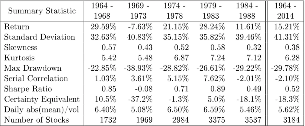
Table 2.1 in the Appendix contains summary statistics for the daily returns in the stock sample. In addition to the statistics for the entire 1964–2014 period, we also provide statistics for consecutive 5-year subperiods (the last subperiod from 2009 to 2014 contains 6 years). As we have posited in Propositions 1 and 2, serial correlation is a very important factor in explaining the performance of tight stop-loss strategies. During the 1964–1988 period, average serial correlation tends to be close to zero or positive. However, from 1989 to 2014, this average is negative over all subperiods. Since average serial correlation is slightly negative over the full period, we expect the historical returns on stop-loss strategies to be inferior to buy-and-hold returns.
We consider two different rates of return on the safe asset. The first is simply 0% all the time; the second is the U.S. 30-day T-bill return. Monthly returns on the T-bill are obtained from Ibbotson Associates and converted to daily returns assuming continuous compounding.
Finally, we incorporate trading costs by assuming that the investor pays one-half of the bid-ask spread whenever a stock is traded, where the spread is calculated with end-of-day closing bid and ask prices from CRSP. However, prior to 1993 these data are missing
approach outlined in Hasbrouck (2009).
1.5.2 Strategy performance
We analyze stop-loss strategies with the stop and start horizons ranging from one day to two weeks. We restrict the start-gain level 𝛿 to values between 0% and 1.5%, and vary the stop level 𝛾 between 0% and −20%. The safe asset is assumed to be the U.S. 30-day
T-bill.5 Figure 1-5 shows strategy performance for the different parameter values.
Tight stop-loss strategies have very poor returns, with the one-day strategy employing a 0% stop losing over −20% per year for all start levels considered, in comparison to the
+15.2% annual gains for the buy-and-hold strategy. This is not surprising since tight
stop-loss strategies require a great deal of trading. Strategies with a wider stop-loss limit provide better performance but still underperform the buy-and-hold strategy in terms of raw returns.
Stop-loss strategies do better when we use the certainty equivalent as the basis of comparison. While most strategies still underperform due to worse returns and higher transaction costs, most strategies employing a wide stop limit do as well as the buy-and-hold or even a little better. In particular, two-week strategies with a start gain level between 0.5% and 1.5%, and stop level between 12% and 16% tend to do best. For these strategies, the CE value is between −14.9% and −16.3%, in comparison to −18.3% for the buy-and-hold. The favorable results stem from the volatility reduction upon employing a stop-loss strategy.
For a mean-variance investor, the buy-and-hold strategy is not necessarily optimal. An investor would tend to allocate only a portion of their wealth to the risky asset, based on the perceived mean and variance of the asset, as well as the individual risk aversion. At the same time, the buy-and-hold strategy is widely used in practice and therefore serves as a natural benchmark when looking at stop-loss strategy performance.
Finally, strategies with wider stops have lower skewness, usually worse than the buy-and-hold, whereas strategies with tight stops have higher skewness and outperform. This is because upside is reduced in all cases. However, performance for tight stop-loss strate-gies is very poor, leading to a significant shift in expected returns and a seemingly shorter left tail. There are quite a few cases when stocks suffer significant intra-day losses, and
Figure 1-5: Historical Stop-Loss Strategy P erfor ma nce, 1964-20 14; U.S. T-bill as Safe Asset BH BH BH BH of stop-loss strategies with varying lev els of stop and start horizons and lev els. The “safe" asset is the U.S. 30-da y statistics are measured usin g ann ual returns and av eraged ou t ov er all years in the sample. The perfromance statisti c for the is in dicated on the colorbar with “BH".
during those cases it is common to observe very high bid-ask spreads (as large as 50% of stock price). This, of course, leads to very poor returns, and in fact quite a few that are worse than −90% over the year, implying a very fat left tail. When it comes to drawdowns, we are able to get improvement over the buy-and-hold strategy, especially when a two-week strategy is used, because the downside is reduced without incurring too much trading cost in the process.
Since many proprietary trading strategies employ tight stops, from now on we focus on strategies with small values for the stop and start levels. We take a “typical" tight stop-loss strategy 𝒮(−2%, 0%, 1, 1) (using the U.S. T-bill as the safe asset) and regress its returns in excess of the buy-and-hold strategy on the statistical properties of stock log returns. We control for the time effect as follows. Each “observation" corresponds to the return on the stop-loss strategy applied to a particular stock in a particular year. We employ indicator variables for each of the 51 years in the sample, excluding the last year to avoid collinearity.
We also control for the firm size effect. On the first day of each of the years in the sample, we compute the market capitalization for each of the available stocks, and split the resulting values into deciles. This way we assign a decile to each stock in each year, and we use indicator variables for each of the ten deciles, again excluding the last one.
To summarize, the regression is: 𝑅𝑆𝑖,𝑡− 𝑅𝐵𝐻
𝑖,𝑡 = 𝛼 + 𝛽𝑥𝑖,𝑡+controls + 𝜖, (16)
where 𝑅𝑆
𝑖,𝑡 is the return on the stop-loss strategy for stock 𝑖 in year 𝑡 and 𝑅𝐵𝐻 is the
return on the buy-and-hold strategy; 𝑥𝑖,𝑡 are various functions of stock returns; controls
are the time and size controls defined earlier; and 𝜖 is a random error term.
Table 1.2 contains the results of the regression. The mean (along with time and size controls) is able to explain a significant portion of variation in returns, around 41.7%.
Adding volatility and the interaction between volatility and mean increases 𝑅2 by about
6.0%. Adding the remaining regressors boosts 𝑅2by another 14.1%, a significant increase.
We next consider a set of regressors motivated by our model for the performance of stop-loss strategies when log-returns follow an autoregressive process. Following Propo-sitions 1 and 2, we only include the mean 𝜇 and the interaction term 𝜌(1) × 𝜎 between the AR(1) coefficient and volatility as the explanatory variables. Table 1.2 shows that
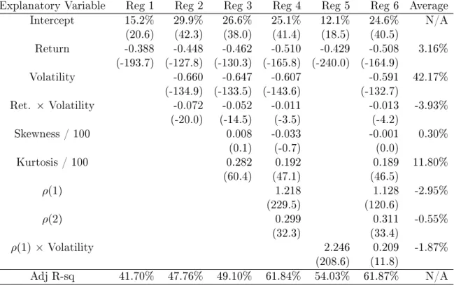
Table 1.2: Regressions of the Stop-loss Strategy 𝒮(−2%, 0%, 1, 1) Relative Return on Statistical Properties of Stock Log Returns
Explanatory Variable Reg 1 Reg 2 Reg 3 Reg 4 Reg 5 Reg 6 Average
Intercept 15.2% 29.9% 26.6% 25.1% 12.1% 24.6% N/A (20.6) (42.3) (38.0) (41.4) (18.5) (40.5) Return -0.388 -0.448 -0.462 -0.510 -0.429 -0.508 3.16% (-193.7) (-127.8) (-130.3) (-165.8) (-240.0) (-164.9) Volatility -0.660 -0.647 -0.607 -0.591 42.17% (-134.9) (-133.5) (-143.6) (-132.7) Ret. × Volatility -0.072 -0.052 -0.011 -0.013 -3.93% (-20.0) (-14.5) (-3.5) (-4.2) Skewness / 100 0.008 -0.033 -0.001 0.30% (0.1) (-0.7) (0.0) Kurtosis / 100 0.282 0.192 0.189 11.80% (60.4) (47.1) (46.5) 𝜌(1) 1.218 1.128 -2.95% (229.5) (120.6) 𝜌(2) 0.299 0.311 -0.55% (32.3) (33.4) 𝜌(1) ×Volatility 2.246 0.209 -1.87% (208.6) (11.8) Adj R-sq 41.70% 47.76% 49.10% 61.84% 54.03% 61.87% N/A
In table 1.2 we regress the return of the stop-loss strategy 𝒮(−2%, 0%, 1, 1) relative to the buy-and-hold strategy on statistical properties of stock log returns. In each regression, we control for time effect and firm size effect by using indicator variables for each year and each market cap decile for the stock at the start of the year. Note that the average value for the log returns is very different than for simple returns in the summary statistics table 2.1 because we are using log returns instead of simple returns.
these two terms explain more than 50% of the variation in returns. Furthermore, the estimated regression coefficients are in line with our model. The coefficient for 𝜇 of −0.43 implies highly negative dependence on the expected return of the underlying process, since higher returns hurt relative performance. The coefficient for the interaction term
𝜌(1) × 𝜎 of 2.2 implies significant dependence on serial correlation and volatility. A more
detailed discussion of why these coefficients are in line with our model is provided in the Appendix.
If we include all eight summary statistics as regressors, the 𝑅2only improves marginally,
suggesting that our model is able to explain the relative performance of tight stop-loss strategies very well, and that this performance has a close to linear dependence on the product of serial correlation and volatility.
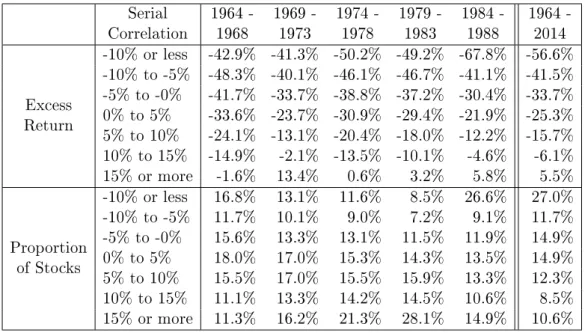
To further investigate the dependence of strategy returns on autocorrelation, in each year we divide the sample of stocks into seven groups based on their realized serial correla-tion for the year. In each group, we compute the return on the 𝒮(−2%, 0%, 1, 1) strategy in excess of the buy-and-hold strategy using the U.S. T-bill as the “safe" asset. Table 1.3 contains the results of this procedure. We find a drastic difference in performance across the realized serial correlation groups. The tight stop-loss strategy applied to stocks with autocorrelation exceeding 15% outperforms the buy-and-hold strategy by 5.5% per year, while it dramatically underperforms by 57% per year for stocks with autocorrelation less than −10%. The overall patterns in this table show that higher autocorrelation leads to significantly better returns. It should be noted that trading costs and positive equity risk premia can cause a tight stop-loss strategy to underperform the buy-and-hold strategy even for stocks with positive serial correlation. The tight stop policy outperforms buy-and-hold only for the stocks in the highest autocorrelation group, and even then only during some of the sub-periods of the entire 1964–2014 sample.
Table 1.3 also contains the excess returns on the strategy in different autocorrelation groups over time. Throughout all of the subperiods, higher autocorrelation gives much better relative performance. The pattern of severe underperformance for stocks with low serial correlation and outperformance for stocks with high serial correlation holds for most subperiods as well.
To develop greater intuition for positive serial correlation in equity returns, we record the proportion of stocks in our sample that fall in a particular serial correlation group
Table 1.3: Returns on the Stop-loss Strategy 𝒮(−2%, 0%, 1, 1) in Excess of the Buy-and-hold Stratified by Serial Correlation
Serial Correlation 1964 -1968 1969 -1973 1974 -1978 1979 -1983 1984 -1988 1964 -2014 Excess Return -10% or less -42.9% -41.3% -50.2% -49.2% -67.8% -56.6% -10% to -5% -48.3% -40.1% -46.1% -46.7% -41.1% -41.5% -5% to -0% -41.7% -33.7% -38.8% -37.2% -30.4% -33.7% 0% to 5% -33.6% -23.7% -30.9% -29.4% -21.9% -25.3% 5% to 10% -24.1% -13.1% -20.4% -18.0% -12.2% -15.7% 10% to 15% -14.9% -2.1% -13.5% -10.1% -4.6% -6.1% 15% or more -1.6% 13.4% 0.6% 3.2% 5.8% 5.5% Proportion of Stocks -10% or less 16.8% 13.1% 11.6% 8.5% 26.6% 27.0% -10% to -5% 11.7% 10.1% 9.0% 7.2% 9.1% 11.7% -5% to -0% 15.6% 13.3% 13.1% 11.5% 11.9% 14.9% 0% to 5% 18.0% 17.0% 15.3% 14.3% 13.5% 14.9% 5% to 10% 15.5% 17.0% 15.5% 15.9% 13.3% 12.3% 10% to 15% 11.1% 13.3% 14.2% 14.5% 10.6% 8.5% 15% or more 11.3% 16.2% 21.3% 28.1% 14.9% 10.6% Serial Correlation 1989 -1993 1994 -1998 1999 -2003 2004 -2008 2009 -2014 1964 -2014 Excess Return -10% or less -87.4% -83.7% -63.6% -36.7% -45.1% -56.6% -10% to -5% -51.1% -57.4% -46.5% -18.9% -22.6% -41.5% -5% to -0% -41.7% -51.8% -40.5% -11.3% -13.8% -33.7% 0% to 5% -32.8% -43.7% -32.7% -3.7% -4.4% -25.3% 5% to 10% -21.5% -35.3% -23.6% 4.3% 3.2% -15.7% 10% to 15% -11.8% -28.3% -8.6% 13.1% 15.1% -6.1% 15% or more 1.8% -20.3% 5.5% 22.3% 20.9% 5.5% Proportion of Stocks -10% or less 40.7% 41.0% 34.1% 30.6% 27.7% 27.0% -10% to -5% 9.2% 11.4% 14.0% 16.7% 17.4% 11.7% -5% to -0% 12.1% 13.5% 16.1% 19.4% 22.1% 14.9% 0% to 5% 12.0% 12.9% 15.2% 16.4% 17.8% 14.9% 5% to 10% 10.9% 10.0% 10.6% 10.0% 9.9% 12.3% 10% to 15% 7.3% 6.0% 5.7% 4.5% 3.7% 8.5% 15% or more 7.8% 5.2% 4.4% 2.4% 1.5% 10.6%
Serial correlation is calculated using daily log returns. Proportion of Stocks measures the pro-portion of stocks in each bucket over the particular period. This is done by calculating the proportion of stocks in a particular bucket for each year and then taking the average over all years. We report results from averaging over all years, as well as over all subperiods. Note that there are more buckets for positive values of serial correlation since these are situations when the stop-loss strategy is more likely to outperform the buy-and-hold strategy.
each year and the striking results are given in Table 1.3. During the first half of the 1964–2014 period, many stocks exhibited high autocorrelation: more than 20% of stocks in each subperiod with correlation exceeding 10%, with as much as 43% of such stocks around 1980. However, over the most recent 25 years, there have been much fewer of these stocks: 15.2% in the 1989–1993 period, and less than that in subsequent periods,
with only 5.2% of such stocks in 2009–2014.6
The pattern is reversed for mean-reverting stocks (i.e., those with low serial correla-tion). In the 1964–1983 period, there were under 20% of stocks with autocorrelation less than −10%. This proportion jumped to 27% in 1984–1988, then to 41% in 1989–1993, and has stayed above 27% in each of the subsequent subperiods. The explanation for this pattern is beyond the scope of this paper. However, as we have demonstrated, using tight stop-loss strategies provides a simple yet effective way to trade serial correlation; thus there is significant economic value in being able to forecast it.
1.5.3 Delayed stop-loss strategies
As documented in Section 1.5.1, daily U.S. stock returns exhibit slight negative au-tocorrelation over the 1964–2014 period, with most of it occurring during the past two decades. This suggests that stocks may have a tendency to revert in the short-term fol-lowing large price movements. This anomaly has been well-documented in the finance literature (e.g., Bremer and Sweeney, 1991; Benou and Richie, 2003; Savor, 2012). As
a result, the delayed stop-loss strategies 𝒮𝑑 may provide superior returns to their
non-delayed counterparts.
Recall that with a delayed stop-loss strategy we wait an extra day to trade out or trade into the risky asset. For example, if the past return over a certain horizon was below a specified threshold on day 𝑡, then the strategy would switch to the safe asset at the end of day 𝑡 + 1 instead of day 𝑡.
Figure 1-6 contains the performance metrics of the delayed stop-loss strategy relative to its non-delayed counterpart using the same specifications. As before, we consider three different past horizon pairs (𝐼, 𝐽), stop-loss levels ranging from 0% to −24%, and start-gain levels between 0% and 1.5%. We see that the delayed strategy provides an
6We calculate these proportions by adding the percentages of stocks in the buckets for correlation
improvement in all cases for the return, CE, and maximum drawdown. The improvement is particularly drastic for the one-day strategy using tight stops, since this is the one for which one-day reversals would be most relevant. For example, one-day strategies using a stop of 0% and start-gain under 1% experience an improvement of 2% to 5% per year when using the delayed specification.
For strategies with wider stops performance gets better when using delays, but it is very marginal. Thus overall, their performance relative to the buy-and-hold would not change drastically, and it would still look similar to Figure 1-5. Finally, we note that delayed strategies usually have better skewness than the non-delayed ones – because upside is more preserved by capturing the positive returns on days following price declines. The only exception is very tight one-day strategies, where skewness decreases; however this is not due to reducing upside, but due to the significant shift in the average (and very negative) strategy return resulting from high transaction costs.
We conclude that using delayed stop-loss strategies marginally improves performance in most cases, and significantly improves returns for the case of tight stops. They are also easier to execute, since the investor can just submit a market-on-close order at the end of the next day rather than trying to submit one right before the close while tracking returns in real-time as with the original stop-loss strategies. Therefore, if an investor does decide to employ stop-loss strategies within our framework, it is generally beneficial to use the delayed specification.
1.6 Optimizing Stop-Loss Level
By now we have a good understanding of how stop-loss strategy performance depends on the underlying market dynamics and strategy parameters. We briefly discuss how to tackle the question of choosing an optimal stop-loss level. We apply the optimization framework to the case of an AR(1) process and investigate how the optimized stop level depends on the process volatility and serial correlation, as well as the investment horizon.
As before, there is a risky asset with log-returns 𝑟𝑡 in period 𝑡, and a risk-free asset
Figure 1-6: Dela yed Stop-Loss Strategy P erformance, 1964-2014 Historical performance of dela yed stop-loss strategies relativ e to the no n-dela yed ones using the same sp ecifications. Relativ e performance is measured by taking differences in the corresp onding performance metrics. The “safe" asset is the U.S. 30-da y T-bill. All statistics are measured using ann ual returns and av eraged out ov er all years in the sample.
There are 𝑇 periods, and therefore 𝑇 + 1 times 0, 1, . . . , 𝑇 . An investor starts with
initial wealth 𝑊0 and can trade at times 𝑡 = 0, 1, . . . , 𝑇 −1 by deciding on allocation 𝑤𝑡+1
during period 𝑡 + 1. His objective is to maximize the expected utility of terminal wealth E(𝑈 (𝑊𝑇)).
At time 𝑡 the investor uses all of the information available up to that point to make
his decision on portfolio allocation 𝑤𝑡+1during the next period. Define by 𝑉 (𝑊𝑡, 𝑤𝑡, ℐ𝑡, 𝑡)
to be the value function which is the expected utility of terminal wealth, conditional on
period 𝑡 wealth 𝑊𝑡, allocation 𝑤𝑡, and information ℐ𝑡 up to time 𝑡. Accounting for the
wealth dynamics, we can write, for 𝑡 = 0, 1, . . . , 𝑇 − 1: 𝑉 (𝑊𝑡, 𝑤𝑡, ℐ𝑡, 𝑡) = max 𝑤∈𝒮 E𝑡[︀𝑉 (𝑊𝑡+1, 𝑤, ℐ𝑡+1, 𝑡 + 1)]︀ 𝑠.𝑡. (17) 𝑊𝑡+1 = 𝑤 × 𝑊𝑡(1 + 𝑟𝑡+1) + [︁ (1 − 𝑤) × 𝑊𝑡− 𝑐 × |𝑤 − 𝑤𝑡| × 𝑊𝑡 ]︁ (1 + 𝑟𝑓)
where 𝒮 is the set of possible values that the allocation can take. After the last period
there is no uncertainty, so that 𝑉 (𝑊𝑇, 𝑤𝑇, ℐ𝑇, 𝑇 ) = 𝑈 (𝑊𝑇). The optimal allocation 𝑤𝑡+1
is defined as: 𝑤𝑡+1* = argmax 𝑤∈𝒮 E 𝑡[︀𝑉 (𝑊𝑡+1, 𝑤, ℐ𝑡+1, 𝑡 + 1) ]︀ (18) subject to the wealth evolution constraint. There have been several popular approaches in the literature for solving the above problem. One “standard" method is Stochastic Dynamic Programming (SDP), outlined, for example, in Infanger (2006). The idea is to calculate the optimal decision function 𝑉 (𝑊𝑡, 𝑤𝑡, ℐ𝑡, 𝑡) recursively for 𝑡 = 𝑇 − 1, . . . , 0 at specified grid points for 𝑊𝑡, 𝑤𝑡, and ℐ𝑡. At each stage 𝑡, and each grid point (𝑊𝑡, 𝑤𝑡, ℐ𝑡) the procedure is as follows. We approximate the conditional expectation function:
𝑓 (𝑤) = E𝑡[︀𝑉 (𝑊𝑡+1, 𝑤, ℐ𝑡+1, 𝑡 + 1) ]︀
(19) by drawing a large sample of next period returns (conditional on current information
ℐ𝑡) and averaging the associated values for 𝑉 (𝑊𝑡+1, 𝑤, ℐ𝑡+1, 𝑡 + 1). These values can be
computed, because we know the value function at the next period gridpoints, and we can interpolate in between.
which would be an approximation for 𝑉 (𝑊𝑡, 𝑤𝑡, ℐ𝑡). After dealing with all the gridpoints at time 𝑡, we move on to time 𝑡 − 1 and repeat.
Brandt et. al (2005) also present an SDP approach, however they propose a novel way
to approximate the optimal solution 𝑤*
𝑡+1. They perform Taylor expansion on the value
function 𝑉 (𝑊𝑡, 𝑤𝑡, ℐ𝑡, 𝑡) and derive the corresponding First Order Conditions. These
produce an expression for the optimal solution as an explicit function of partial derivatives of the value function in the next period. The advantage of this approach is that it can
deal with more complicated dynamics for the evolution of information ℐ𝑡 than other
simulation-based methods.
Finally, Moallemi and Sağlam (2015) demonstrate how to solve the above problem when considering only the space of linear dynamic policies. That is, the next period
allocation 𝑤𝑡 is restricted to be a linear function of the previous allocation 𝑤𝑡−1 and
factors 𝑓𝑠 that make up the information set ℐ𝑡. The authors demonstrate that in that
case they can optimize over all periods 𝑡 = 0, 1, . . . , 𝑇 − 1 at once in a single convex optimization problem. The method is shown to be tractable and provides near optimal results.
1.6.1 Applying SDP to Stop-Loss Problem
We now go into more detail about how to solve the optimization problem (17) in the context of our framework. As before, suppose there are two assets: the risky asset with a
return 𝑟𝑡during period 𝑡 and the risk-free asset yielding a constant return 𝑟𝑓 each period.
The risky asset log returns ˜𝑟𝑡 follow an AR(1) process:
˜
𝑟𝑡+1 = 𝜇 + 𝜌(˜𝑟𝑡− 𝜇) + 𝜎𝜖𝑡, 𝜖𝑡∼ 𝑊 𝑁 (0, 1) (20)
where 𝜇 is the mean, 𝜎 is the volatility, and 𝜌 is the serial correlation coefficient. We assume the investor knows this is indeed the right model and also its parameters 𝜇, 𝜎,
and 𝜌. At the end of each period 𝑡 = 0, 1, . . . , 𝑇 − 1 he is able to observe the return 𝑟𝑡 for
that period (as well as the previous periods); he chooses his allocation 𝑤𝑡+1 for the next
period.
The investor chooses his allocation using the forecast distribution 𝑟𝑡+1|ℐ𝑡 conditional
process and the investor knows this, then it suffices for him to just consider the return in
the previous period and look at the corresponding distribution 𝑟𝑡+1|𝑟𝑡. This significantly
reduces the dimensionality of the problem.
We assume the investor has initial wealth 𝑊0 and has a quadratic utility function
𝑈 (𝑊 ) = 𝑊 − 𝜆𝑊2. The allocations in each period are restricted to be either 0% or
100%.
We are now ready to solve (17) using approximate SDP. We first create a grid of nodes
(𝑊𝑡, 𝑤𝑡, 𝑟𝑡) for each time 𝑡. For allocation 𝑤𝑡 we consider just the values 0% and 100%
(since these are all the possible allocations the investor can use).We consider 100 evenly
spaced values for log returns ˜𝑟𝑡 in the range [𝜇 − 𝑘 ×𝜎, 𝜇 + 𝑘 ×̂︀ ̂︀𝜎], where 𝑘 is a scaling
factor and 𝜎 = 𝜎/√︀1 − 𝜌̂︀
2 is the unconditional volatility of the AR(1) process. With
𝑘 = 3, about 99.7% of the log return values sampled under the unconditional distribution
will fall into the interval we use, which is very good coverage. From the log returns we easily obtain simple returns 𝑟𝑡 as 𝑟𝑡= exp(˜𝑟𝑡) − 1.
For wealth 𝑊𝑡 we consider 101 equally spaced values in the range [𝑊0exp(𝜇𝑡 − 𝑘𝜎
√ 𝑡,
𝑊0exp(𝜇𝑡 + 𝑘𝜎
√
𝑡)], where 𝑘 is again the scaling factor. Note that this range increases
with 𝑡 to accommodate for the fact that as time passes, the distribution of values of wealth becomes more and more dispersed. The motivation for the functional form of the bounds comes from the evolution of Geometric Brownian Motion after time 𝑡, assuming drift 𝜇 and volatility 𝜎. Of course, here things are a bit more complicated due to the serial correlation 𝜌 in returns; however for a small value of 𝜌 (under 20% in absolute value) and a large value of 𝑘 (we use 𝑘 = 3) we will again be covering a large proportion of the sample of possible values of wealth. Note that Brandt et al. (2006) use the same functional form.
Within this set of values 𝑊𝑡 we insert another value of 𝑊0, in order to compare the
optimal stop-loss level as a function of investment horizon, while keeping initial wealth
constant. Thus in the end we use 102 values of 𝑊𝑡 in the nodes at each time 𝑡.
Once the nodes are well-defined, we outline how to do optimization at each node. We solve the optimization problem recursively at all nodes at time 𝑇 − 1, then at all nodes
function:
𝑉 (𝑊𝑡+1, 𝑤𝑡+1, 𝑟𝑡+1) = 𝑉 (𝑊𝑇, 𝑤𝑇, 𝑟𝑇) = 𝑈 (𝑊𝑇) = 𝑊𝑇 − 𝜆𝑊𝑇2 (21)
As discussed in the previous section, we need to calculate the conditional expectation
function 𝑓(𝑤) in (19), where we condition on past period return 𝑟𝑡. To do this, we resort
to a “direct" density approximation, where we take 100 evenly spaced values ˜𝑟𝑡+1,𝑠 in the
range [𝜇𝑐− 𝑘 × 𝜎𝑐, 𝜇𝑐+ 𝑘 × 𝜎𝑐], where 𝑘 = 3 is a scaling factor giving very good coverage
of the distribution, and 𝜇𝑐, 𝜎𝑐 are the parameters for the conditional distribution of ˜𝑟𝑡+1:
˜
𝑟𝑡+1|˜𝑟𝑡∼ 𝑁 (𝜇𝑐, 𝜎𝑐2); 𝜇𝑐= 𝜇 + 𝜌(˜𝑟𝑡− 𝜇), 𝜎𝑐= 𝜎
For each of the values ˜𝑟𝑡+1,𝑠 we calculate the next period wealth 𝑊𝑡+1 and the
corre-sponding value function 𝑉 as in (21). These are then combined using a weighted average,
where the weights correspond to the densities for ˜𝑟𝑡+1,𝑠 under the distribution 𝑁(𝜇𝑐, 𝜎𝑐2),
and scaled to add to 100%. This gives us 𝑓(𝑤).
The final step is optimization. This is easy, because we know 𝑤 ∈ {0%, 100%}, so it suffices to just calculate 𝑓(0%) and 𝑓(100%) and take the larger value.
Case 2: 𝑡 ≤ 𝑇 − 2. In this case we know the value function 𝑉 (𝑊𝑡+1, 𝑤𝑡+1, 𝑟𝑡+1) at
specific nodes in the next period. We carry out the exact same procedure as in Case 1 by
calculating next period wealth 𝑊𝑡+1 for each value ˜𝑟𝑡+1,𝑠. The only new part is that the
next period triplet (𝑊𝑡+1, 𝑤𝑡+1, 𝑟𝑡+1)may not hit an exact node in the next period. If that
happens, we perform interpolation between the nodes (we resort to linear interpolation).
Note that we need to only interpolate over (𝑊𝑡+1, 𝑟𝑡+1)because 𝑤𝑡+1∈ {0%, 100%} gives
us full coverage of all the possible values for 𝑤. After performing the interpolation we can calculate 𝑓(𝑤) and again optimize.
1.6.2 Optimization Results
We apply the above optimization approach to an investment problem with a horizon
of 𝑇 = 20 periods. We assume each period is a month7.The annual mean is assumed to be
10%, and we consider different cases for annualized volatility, ranging from 10% to 50%.
We also consider different cases for the serial correlation 𝜌, in the range [−20%, 20%]. These parameters are the same as in the simulations for an AR(1) process we carried out