Did the Clean Air Act Cause the Remarkable Decline in Sulfur Dioxide Concentrations? by 04-007 October 2003 Michael Greenstone WP
Did the Clean Air Act Cause the Remarkable Decline in Sulfur Dioxide Concentrations?*
Michael Greenstone MIT Department of Economics
50 Memorial Drive, E-52 Cambridge MA 02142-1347 American Bar Foundation and NBER
mgreenst@mit.edu ph: 617-452-4127 fax: 617-253-1330
October 21, 2003
* The careful comments of Joseph Herriges and three anonymous reviewers substantially improved this paper. Spencer Banzhaf, Gib Metcalf, and the participants at the NBER conference “Empirical Advances in Environmental Economics” provided numerous insightful remarks. I thank Katherine Ozment for many informative conversations. Matthew Witosky of the EPA Region 6 Office deserves special thanks for enlightening conversations about SO2 nonattainment policies. Justin Gallagher, Paulette Kamenecka,
Did the Clean Air Act Cause the Remarkable Decline in Sulfur Dioxide Concentrations? ABSTRACT
Over the last three decades, ambient concentrations of sulfur dioxide (SO2) air pollution have declined by
approximately 80%. This paper tests whether the 1970 Clean Air Act and its subsequent amendments caused this decline. The centerpiece of this legislation is the annual assignment of all counties to SO2
nonattainment or attainment categories. Polluters face stricter regulations in nonattainment counties. There are two primary findings. First, regulators pay little attention to the statutory selection rule in their assignment of the SO2 nonattainment designations. Second, SO2 nonattainment status is associated with
modest reductions in SO2 air pollution, but a null hypothesis of zero effect generally cannot be rejected.
This finding holds whether the estimated effect is obtained with linear adjustment or propensity score matching. Overall, the evidence suggests that the nonattainment designation played a minor role in the dramatic reduction of SO2 concentrations over the last 30 years.
JEL Classification: Q25; Q28; H22; H11
I. Introduction
Prior to 1970, states, counties, and municipalities were principally responsible for environmental regulations. In one of the most significant government interventions into the marketplace of the post-World War II era, the federal government made a dramatic foray into the regulation of air pollution with the passage of the Clean Air Act Amendments (CAAAs) and the establishment of the Environmental Protection Agency (EPA) in 1970. Congress further strengthened the provisions of the CAAAs in 1977 and 1990.
The CAAAs are controversial, because reliable evidence on their costs and benefits is not readily available. For instance, there is not even a consensus on whether the CAAAs are responsible for the dramatic improvements in air quality that have occurred in the last 30 years [6, 7, 11, 16, 24]. The fundamental problem is that there is not a valid counterfactual for what would have happened to air quality concentrations in the absence of these regulations.
This paper exploits the structure of the CAAAs to determine whether this legislation is responsible for the remarkable 80% decline in national sulfur dioxide (SO2) concentrations from .0301
ppm in 1970 to .0048 ppm in 1992.1 The centerpiece of this legislation is the establishment of the National Ambient Air Quality Standards (NAAQS) – a minimum level of air quality that all counties are required to meet – for SO2 and six other pollutants.2 As a part of this legislation, each U.S. county
annually receives separate nonattainment or attainment regulation designations for each of the pollutants. The nonattainment designation is reserved for counties whose air contains concentrations of the relevant pollutant that exceed the federal standard. Emitters of the controlled pollutant in nonattainment counties are subject to greater regulatory oversight than emitters in attainment counties.
1 These figures are not based on a fixed set of monitors but nevertheless are illustrative of the long-run
decline in SO2 concentrations.
2 The other pollutants are carbon monoxide, lead, nitrogen dioxide, ozone, small particulate matter, and
This paper empirically tests whether SO2 nonattainment status caused a reduction in SO2
concentrations relative to attainment status.3 This is an interesting test, because the primary aim of the CAAAs was to bring all counties into compliance with the federal standards. It is important to note from the outset though that the results are not directly informative about the CAAAs’ effect on nationwide air quality, because this legislation also introduced regulations in attainment counties.
The analysis is conducted with comprehensive county-level data files on SO2 concentrations,
nonattainment designations, and economic activity for the 1969-1997 period. Through a Freedom of Information Act request, I obtained summary information on the universe of state and national SO2
monitors from the EPA. Although the SO2 attainment/nonattainment status of each county is central to
federal environmental law, this is the first study to collect them (from the Code of Federal Regulations) and use this information during this key period. The pollution and regulation data are merged to county-level economic data from the Bureau of Economic Analysis.
An immediate, yet surprising, finding is that the vast majority of nonattainment counties had pollution concentrations below, in many cases substantially so, the federal SO2 standard. Despite
extensive communications with the EPA, I am unable to conclusively determine why they received this designation. Thus, this paper attempts to evaluate the impact of SO2 nonattainment status when the
selection rule is unknown. The evaluation problem is made even more difficult by the finding that in the “pre-period” nonattainment counties have higher SO2 concentrations and larger downward trends in
ambient SO2 than the attainment counties.
To control for the likely confounding due to these observable differences, linear regression and propensity score matching techniques [20] are employed to estimate the effect of SO2 nonattainment
status in three different 6-year periods, 1975-80, 1981-86, and 1987-92. The analysis reveals that
3 A number of recent studies have employed similar econometric strategies: Becker and Henderson [3],
Greenstone [12], and Henderson [16] examine the relationship between nonattainment status and manufacturing activity; Henderson [16] documents the relationship between ozone nonattainment status and ozone concentrations; Chay and Greenstone [6] explore the impact of TSPs nonattainment status on TSPs concentrations and housing prices; and Chay and Greenstone [7] assess the effects of TSPs nonattainment status on TSPs concentrations and infant mortality rates.
matching is especially useful when the observable differences between the nonattainment and attainment counties are greatest. The results indicate that SO2 nonattainment status is associated with modest
reductions in SO2 air pollution, but a null hypothesis of zero effect generally cannot be rejected. Overall,
the paper finds that the nonattainment designation played a minor role in the dramatic reduction of SO2
concentrations over the last three decades.
The paper proceeds as follows. Section II describes the structure of the CAAAs and provides some background information on sulfur dioxide pollution. Section III discusses the data sources and presents some summary statistics. Section IV describes the research design and some of the challenges to its validity. Section V presents the econometric strategy and Section VI discusses the results. The paper ends with brief interpretation and conclusion sections.
II. Background on the Evolution of Air Pollution Law and Sulfur Dioxide Pollution
The ideal analysis of the relationship between air pollution and environmental regulations would involve a controlled experiment in which the regulations are randomly assigned. In this case, regulatory status is independent of all other determinants of air quality. Consequently, the subsequent differences in air quality can be causally related to the regulations. In the absence of such an experiment, an appealing alternative is to find a case where the assignment of regulation differs across similar counties. The structure of the CAAAs may provide such an opportunity. This section describes the CAAAs and the opportunity that they may provide to credibly identify the relationship between clean air regulations and sulfur dioxide concentrations. It also briefly reviews sulfur dioxide pollution and its consequences.
A. The CAAAs and Nonattainment Status
The centerpiece of the CAAAs is the establishment of separate National Ambient Air Quality Standards (NAAQS) for SO2 and other “criteria” air pollutants, which all counties are required to meet.4
For SO2 pollution, a county is in violation of the standards if: 1) its annual mean concentration exceeds
goal of the CAAAs is to bring all counties into compliance with these standards by reducing local air pollution concentrations. To achieve this goal, stricter regulations are imposed on emitters in nonattainment counties than in attainment ones.
The EPA annually assigns separate nonattainment-attainment designations for each of the criteria pollutants. The nonattainment designation is supposed to be reserved for counties whose actual or modeled air pollution concentration exceeds the federal ceiling. Generally, this determination is based on the previous year’s actual or modeled air pollution concentration. Chay and Greenstone [6, 7] and Henderson [16] document the effectiveness of nonattainment status in reducing total suspended particulates and ozone air pollution, respectively. The current study empirically tests the effect of nonattainment status on SO2 concentrations relative to attainment status.
B. Background on Sulfur Dioxide Pollution
Sulfur dioxide is a colorless gas, which is odorless at low concentrations but pungent at very high levels. It results naturally from sources such as volcanoes and decaying organic material. Human activity accounts for approximately 100 million tons SO2 per year. The primary man-made source of SO2 is from
the combustion of fuels (e.g. coal and oil) that contain sulfur. The largest industrial emitters of SO2 are
the electric utility plants that use cheaper high sulfur coal from the eastern U.S. In the manufacturing sector, the largest emitters are petroleum refineries, smelters, paper mills, chemical plants, and producers of stone, clay, glass, and concrete products.
SO2 has a number of unwanted effects. It is one of the major contributors to smog. At high
levels, it can affect the respiratory system (especially among asthmatics), weaken the lung’s defenses, aggravate existing respiratory and cardiovascular diseases, and potentially even lead to premature death [23].5 At much lower levels, it damages trees and agricultural crops. Along with nitrous oxides, SO
2 is
the major contributor to the formation of acid rain.
4 See Lave and Omenn [17] and Liroff [18] for more detailed histories of the CAAAs.
III. Data and Overview of Trends in Sulfur Dioxide Concentrations and Regulation
To implement the analysis, I compiled the most detailed and comprehensive data available on SO2 concentrations and nonattainment status. This section describes the data and its sources and presents
summary statistics on national trends in SO2 monitoring, concentrations, and regulation. A. SO2 and Regulation Data
The SO2 concentration data were obtained by filing a Freedom of Information Act request with
the EPA. This yielded the Quick Look Report data file, which is derived from the EPA’s Air Quality
Subsystem database. For each SO2 monitor operating at any point in the 1969-1997 period, the file
contains annual information on the number of recorded hourly readings, the average across all these readings, and the two highest readings for 1, 3, and 24 hour periods. It also reports the monitor’s county.
Annual county-level SO2 concentrations are calculated as the weighted average of the annual
arithmetic means of each monitor in the county, with the number of observations per monitor used as weights. In practice, I calculate this from the set of monitors that operated for at least 75% of the year (i.e., 6,570 hours). These monitors meet the EPA’s minimum summary criterion and this sample restriction is applied in throughout the analysis.6
The annual county-level SO2 nonattainment designations were determined from the annual Code of Federal Regulations (CFR). For each of the criteria pollutants, the CFR lists every county as, “does
not meet primary standards,” “does not meet secondary standards,” “cannot be classified,” “better than national standards,” or “cannot be classified or better than national standards.” Additionally, the CFR occasionally indicates that only part of a county did not meet the primary standards. I assigned a county to the SO2 nonattainment category if all or part of it failed to meet the SO2 “primary standards”; 5 See Chay, Dobkin, and Greenstone [5], Chay and Greenstone [7, 8], Dockery et al. [10], and Ransom
and Pope III [19] on the relationship between air pollution and human health.
6 To preclude the possibility that counties or states place monitors to produce false pollution
concentrations, the Code of Federal Regulations contains precise criteria that govern the siting of a monitor. Among the most important criteria is that the monitors capture representative pollution concentrations in the most densely populated areas of a county. Moreover, the EPA must approve the location of all monitors and requires documentation that the monitors are actually placed in the approved
otherwise, I designated it attainment. These annual, county-level, designations were hand entered for the 3,063 U.S. counties for the years 1978-1992. Although these designations were applied before 1978, the identity of the nonattainment counties is unavailable from earlier CFRs and the EPA. This poses some difficulties for the analysis, because it means that there is no “pre-period” where the regulations are not in force. This issue is discussed further below.
B. National Trends in SO2 Monitoring, Concentrations, and Regulation
Table I presents annual summary information from the SO2 monitor and nonattainment data.
Column (1) reports the number of monitors that meet the EPA’s minimum summary criteria. Columns (2) and (3) present the number of counties in which these monitors are located and their population. The passage of the 1970 CAAAs led to an extensive program to site monitors around the U.S. and obtain better readings of the prevailing SO2 concentrations. Since the late 1970s, the number of operating
monitors has varied between approximately 500 and 650. These monitors are spread out over approximately 300 counties, implying that on average there are slightly less than 2 monitors operating in each county.7 From 1980 onward, the population in counties monitored for SO
2 ranges between 110 and
125 million, demonstrating that the monitoring program was focused on the most heavily populated of the more than 3,000 U.S. counties.
Although the total number of monitored counties is roughly constant after the late 1970s, there is a lot of churning in the set of monitored counties. For example, 576 different counties are monitored over the 1969-97 period. Since the monitoring program is aimed at the dirtiest counties, the EPA and the states generally remove monitors from counties that become “clean” and add monitors in “dirty” counties. In order to avoid any biases associated with compositional changes, the subsequent tests of the effect of nonattainment status on SO2 concentrations are conducted on fixed sets of counties. In the presence of
locations. This information is derived results from the Code of Federal Regulations 1995, title 40, part 58 and a conversation with Manny Aquilania and Bob Palorino of the EPA’s District 9 Regional Office.
7 In the vast majority of counties, only 1 monitor records SO
2 concentrations. However, in large,
industrial counties, such as Los Angeles, CA, Cook (Chicago), IL, and Wayne (Detroit), MI, it is not uncommon for more than 10 monitors to operate simultaneously.
the churning, however, this restriction means that there is a tension between the number of years and counties in any sample.
Columns (4) and (5) report the unweighted and weighted (where county population is the weight) mean annual concentration across all operating monitors. Column (6) lists the annual means of the 2nd
highest 24-hour county-level readings. Each county’s 2nd highest reading is the maximum of the 2nd
highest daily readings across all monitors (not just those that meet the minimum summary criteria) within a county by year and the entry is the unweighted mean of these readings.
All three measures reveal a dramatic decline in SO2 concentrations in the last 30 years. For
example, the unweighted (population weighted) annual average declined from .0380 ppm (.0359 ppm) in 1969 to .0105 (.0098) in 1980 and then to .0048 (.0050) in 1997. The extreme concentration readings follow a similar pattern. It is evident that the national average SO2 concentration was well below the
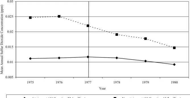
federal standards by the mid-1970s. Figure 1 graphically displays the SO2 trends and the population in
monitored counties. In light of the similarity in the unweighted and weighted concentrations, the subsequent analysis exclusively uses the unweighted measures.
Columns (7)-(9) report the number of counties with monitor readings exceeding the annual, daily, or either federal standard. All of these measures exhibit a strong downward trend. In fact since 1981, fewer than 10 of the monitored counties exceeded the SO2 NAAQS in any year. And since 1986, it is
fewer than 5.
Columns (10) and (11) list the number of counties designated nonattainment in the CFRs. The former column reports this information among the set of monitored counties, while the latter column reports it for all counties.8 The number of nonattainment counties always greatly exceeds the number of
8 A comparison of the two columns reveals that many counties that do not meet the criterion for sufficient
monitoring are designated SO2 nonattainment. Presumably, the EPA’s models indicate that these counties
counties exceeding the SO2 NAAQS in the previous year. In fact a number of the nonattainment counties
had not exceeded the standard for many years.9
It is evident that SO2, nonattainment status is not mechanically assigned according to whether a
county violates the NAAQS. This finding greatly complicates an evaluation of the effect of nonattainment status on SO2 concentrations. Since the NAAQS specify the selection rule that in principle
determines nonattainment status, it is natural to evaluate this program with a regression discontinuity approach as in Chay and Greenstone [6, 7]. Such an evaluation technique relies on the assumption that counties just above and below the NAAQS threshold are virtually identical and that comparisons near the threshold will produce unbiased estimates of the effect of nonattainment status on air pollution concentrations.
This section’s findings reveal that the selection rule for the SO2 nonattainment designation is
unknown, so it is not appropriate to use a regression discontinuity design here. Consequently, the validity of the subsequent analysis turns on the successfulness of adjusting for the heterogeneity across nonattainment and attainment counties. This is the subject of the remainder of the paper.
IV. The Research Design and Challenges to Its Validity A. Research Design
This paper conducts separate analyses of the impact of SO2 nonattainment status on SO2 air
pollution in 3 non-overlapping periods, 1975-1980, 1981-1986, and 1987-1992. In order to be included in the sample for a period, a county must have at least one monitor that meets the minimum summary criteria in every year of that period.10 The extension of the sample beyond 6 years causes the sample sizes
9 As an example, the paper examines 19 counties that are designated SO
2 nonattainment in 1990. 12 of
these 19 counties did not exceed the NAAQS in any of the previous 10 years.
10 The advantage of fixing the sample is that it avoids any biases associated with changes in the
composition of monitored counties. The disadvantage is that the EPA’s decision to stop monitoring a county may be associated with nonattainment status. In particular, the nonattainment regulations may reduce SO2 concentrations and the EPA may systematically cease monitoring the counties with these
improvements in air quality. In this case, this paper’s use of a fixed sample approach will cause the effect of the nonattainment designation to be biased upward.
to deteriorate rapidly. Further, due to the small number of monitored counties in the early 1970s, it is not practical to begin the analysis until 1975, 5 years after the passage of the 1970s CAAAs.
The paper tests the effect of the nonattainment designation that is assigned in the 4th year of each period. Since the nonattainment designation is supposed to be based on the previous year’s pollution concentration the third year is henceforth referred to the “regulation selection year” or year “t-1”. Thus, each period contains 3 years before the assignment of this designation and 3 years subsequent to it. The 3 “pre-period” years are used to adjust for differences across the nonattainment and attainment counties. The CAAAs frequently require the implementation of abatement activities over a period of a few years and the 3 “post-period” years allow the effect to vary over time.
B. Pre-Period Differences in Attainment and Nonattainment Counties
Since the nonattainment designation is not assigned randomly, this subsection examines the association between nonattainment status and the likely determinants of changes in SO2 concentrations in
the post-period. Because the CAAAs require the assignment of nonattainment status to be based on SO2
concentrations, it is to be expected that there are differences across the categories of counties. The identification of these differences is important, because it reveals the sources of heterogeneity that must be adjusted for in order to avoid confounding the effect of nonattainment status with them.
Table II explores some of these sources of heterogeneity. Each 6-year period is examined in a separate panel. Columns (1) and (2) detail the number of counties and their populations in each period. Columns (3a)-(3e) report the mean SO2 concentration in the regulation selection year (i.e., 1977, 1983,
and 1989), the change between t-1 and t-3, and the number of counties exceeding the SO2 NAAQS in
each of the pre-period years, respectively.
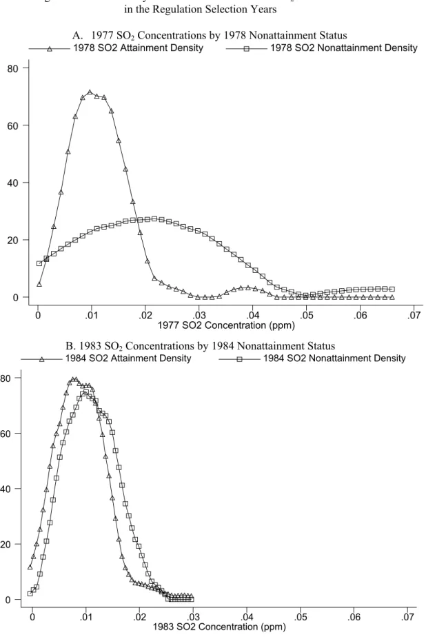
Figures 2 and 3 graphically describe the pre-period heterogeneity. Figure 2 plots the annual SO2
concentrations by nonattainment status. The points to the right of the vertical line are the post-period years. Figure 3 presents separate kernel density plots of the distribution of SO2 concentrations in the
regulation selection year for nonattainment and attainment counties. Both figures include separate panels for each period.
1975-80. This period is structured to take advantage of the first publication of the nonattainment
designations in 1978. It may be an especially interesting period, because it allows for a test of nonattainment status in the first year that the 1977 CAAAs were in force. There are 44 attainment and 18 nonattainment counties, with populations of 23.6 and 15.7 million, respectively. A simple before and after comparison suggests that nonattainment status reduced SO2 concentrations.
There are at least two important differences in the pre-period concentrations of SO2. First, mean
SO2 concentrations are roughly two times higher in nonattainment counties. From the kernel density plots
in Figure 3A, it is evident that this mean difference is not due to a few outliers. In particular, there are few attainment counties with concentrations in the range covered by the majority of the nonattainment distribution. Second, there is a downward trend in the nonattainment counties in the pre-period, while concentrations are essentially flat in the attainment ones.
Columns (3c)-(3e) of Table II reveal that only 7 of the 18 counties designated nonattainment met the statutory requirements necessary for this designation. Among the attainment counties, only 1 of them exceeds the federal standards. Overall, it is evident that the practical selection rule for nonattainment status differed from the statutory one.
In summary, Figure 2A suggests that 1978 nonattainment status reduced SO2 concentrations, but
a closer examination of the data leads to a less certain conclusion. In particular, it is possible that the observable differences among attainment and nonattainment counties or the unobserved variables that determine the selection rule for nonattainment status explain the relative post-period decline in nonattainment counties. It is evident that in order to obtain a consistent estimate of nonattainment status, the subsequent analysis will need to successfully adjust for these factors.
1981-86. The 1980s are often regarded as a period when environmental regulations were not
enforced vigorously. This period provides an opportunity to empirically test this hypothesis. There are 139 counties with 76.3 million people in the 1984 attainment category and 23 counties with a combined population of 9.7 million in the nonattainment one. In the years in which 1984 nonattainment status applied, the nonattainment counties have a slightly larger decline in SO2.
Again, there are important pre-period characteristics of the counties that vary with nonattainment status. For example, the regulation selection year mean SO2 concentrations are higher in nonattainment
counties. Also, the pre-period decline is greater in the nonattainment counties (roughly .0037 ppm versus .0008 ppm). Notably, only 1 of the nonattainment counties exceeded the SO2 NAAQS in the regulation
selection year. This finding is salient because it indicates that the statutory selection rule did not determine the assignment of SO2 nonattainment in this period too. This reinforces the point that a
regression discontinuity evaluation strategy is not appropriate.
1987-92. This period allows for a test of the effect of nonattainment status in the first years in
which the 1990 CAAAs were in force. There are 184 counties with a population of 87.4 million in the 1990 attainment category and 19 counties with approximately 7.7 million people in the nonattainment group. Together these counties accounted for approximately 40% of the U.S. population in this period. Figure 2C reveals an association between nonattainment status and a post-period reduction in SO2
concentrations.
However, there are substantial pre-period differences in the two sets of counties. In the nonattainment counties during the pre-period, SO2 concentrations are higher and there is a larger
downward trend. Further, the rule that determines nonattainment status remains a mystery. It appears likely that just as in the other periods, a simple pre and post comparison will not reveal the causal effect of nonattainment status on SO2 concentrations.
C. Intra-County Variation in Nonattainment Status
An important issue for this analysis is that there is little intra-county variation in counties’ attainment-nonattainment designation over time. This is because few counties’ nonattainment status changed after 1978. The last three columns of Table II demonstrate this point in the three periods examined here. Columns (4a) (4b), and (4c) report the number of counties designated nonattainment in any of the pre-period years (i.e., t-1, t-2, and t-3), all the pre-period years, and in all years from 1978 through year t-1, respectively. Column (4b) reveals that almost all counties that are nonattainment in the 4th year of the 1981-6 and 1987-92 periods are also nonattainment throughout the pre-period. Further, 20
(13) of 23 (19) 1984 (1990) SO2 nonattainment counties were also nonattainment in every year from 1978
through the regulation selection year. Interestingly, a small, but nontrivial, fraction of the attainment counties were previously designated nonattainment.
The absence of time variation in nonattainment status has a number of important implications. First, the “pre-period” years are not before the counties are regulated, but simply before the arbitrarily chosen 1978, 1984, and 1990 nonattainment designations that this paper evaluates. For ease of exposition, I use “pre” and “post” throughout the remainder of the paper but note that their meaning here differs from the standard definitions.
Second, although it would be interesting to determine whether there is heterogeneity in the effect of nonattainment status, it will be difficult to investigate some likely sources. For example, the effect might vary with the number of years that a county has been designated nonattainment (i.e., the effect on SO2 concentrations may be greater in the 1st year that a county is nonattainment than in the 9th year).
Alternatively, the EPA’s enforcement intensity may vary with the political climate. Unfortunately, it is impossible to separately identify these two potential sources of heterogeneity because almost all counties that were ever nonattainment were first designated nonattainment in 1978. The subsequent analysis allows the effect of nonattainment status to differ in each of the three periods but whether any differences are due to the length of time that a county was designated nonattainment or the President’s preferences about the environment cannot be assessed.
Third, and most importantly, the analysis is structured to evaluate the effect of the nonattainment designation assigned in the 4th year of each period, but this interpretation of the estimated effects may not be valid. Although linear regression and propensity score matching are used to adjust for the pre-period differences (e.g., in SO2 concentrations) between the nonattainment and attainment counties, the absence
of within county variation in nonattainment status means that it is impossible to directly control for pre-period differences in the incidence of the nonattainment designation. Consequently, it may be more appropriate to interpret the estimated treatment effect as a measure of the effect of a county being
designated nonattainment over a longer period, rather than the effect of the 4th year’s nonattainment designation.
V. Econometric Strategies
This paper utilizes a variety of statistical models to control for the differences between attainment and nonattainment counties that were documented in the previous section. Here, I describe these econometric strategies.
First Differences. The first differences strategy is based on the assumption that any differences in
SO2 concentrations between the two sets of counties are due to permanent factors (e.g., a county’s
topography) that have time invariant effects on SO2 pollution. Let Di4 be an indicator variable that equals
1 when county i is designated nonattainment in the 4th year of one of the 6 year periods and 0 if it is
attainment. Now, consider: (1) Yit - Yi3 = θt + αtDi4 + ηit,
where t denotes the year and 4 <= t <= 6, indicating that the dependent variable is the change in SO2
concentrations between the 4th, 5th, or 6th year and the 3rd year. θ
t is a nonparametric time effect that is
common to attainment and nonattainment counties and ηit is the idiosyncratic unobserved component of
the change in SO2 concentrations.
αt is the parameter of interest and measures the difference in the change in SO2 concentrations
between nonattainment and attainment counties. Formally, αt = E[Yit - Yi3|Di4=1] - E[Yit - Yi3|Di4=0].
Equation (1) is estimated separately for each of the post-period years and the t subscript on α highlights that the effect of nonattainment status is allowed to vary across years within a period.11 For example, it may be of a larger magnitude in the 6th year of a period (e.g., 1980) than in the 4th (e.g., 1978). Notably,
the differencing removes the time-invariant characteristics that are the only source of bias under this model’s assumptions.
11 For example in the 1975-80 period, I separately estimate (1) when the dependent variables are Y i1978 -
The mapping that assigns a value to the nonattainment indicator merits further discussion. This mapping emphasizes that the aim of this exercise is to evaluate the effect of the 4th year nonattainment designation. The difficulty is that the pre-period SO2 nonattainment designations are highly correlated
with Di4. This correlation will cause the estimated αt to capture the effect of the 4th year nonattainment
designation and the effect of the pre-period SO2 nonattainment designations. The point is that it is likely
to be incorrect to interpret αt as the effect of the 4th year nonattainment designation only.
A more troubling possibility is that the identifying assumptions of this model are unlikely to be valid. This is because the nonattainment designation is highly correlated with past pollution levels, which in turn are likely correlated with current pollution levels through ηit. This would be the case if, for
example, there is mean reversion in SO2 concentrations. Moreover, the differential pre-period trends in
SO2 concentrations documented in Section IV are likely to cause a correlation between Di4 and ηit. Such
unwanted correlations will bias the estimated effect of nonattainment status, αt.
Adjusted First Differences. In light of these issues, the paper also linearly adjusts for the
heterogeneity across attainment and nonattainment counties. The model is: (2) Yit - Yi3 = θt + Xib’β + Pib’φ + αtDi4 + ηit,
where the b subscript indicates the pre-period. The substantive difference with equation (1) is that here the estimated effect of nonattainment status on the change in SO2 concentrations is conditional on linear
adjustment for the vectors Xib and Pib.
In practice, Xib includes nonattainment status for carbon monoxide, ozone, and total suspended
particulates in the same year that Di4 is measured (i.e., 1978, 1984, and 1990). As Table II demonstrated,
there is little within county variation in SO2 nonattainment status, so it is not practical to include measures
of this variable from earlier years. The vector also includes county-level measures of per capita income, the average wage, total employment, and total population.12 Moreover in some specifications, X
ib
includes a full set of state fixed effects so that the estimated treatment effect is based on intra-state comparisons of SO2 attainment and nonattainment counties.
Pib is a vector that includes a number of measures of lagged SO2 pollution concentrations in order
to break the unwanted correlation between Di4 and ηit. For instance, it includes the mean SO2
concentration from the t-2 and t-3 pre-period years (e.g., 1976 and 1975 in the 1975-80 period). The vector also includes the annual maximum 1 hour, 3 hour, and 24 hour readings from t-1, the regulation selection year. Since the correct functional form for the lagged SO2 pollution variables is unknown, some
specifications will include squares and cubes of these variables.
Here, the identifying assumption is that
E[
Di4 ηit|
Xib, Pib, θt] = 0 or that
4th year nonattainmentstatus is independent of potential pollution concentrations, conditional on the covariates. Recall, the EPA’s exact selection rule is unknown but it seems sensible to assume that it is a function of lagged pollution levels, economic activity, and its cognizance of a county’s overall air quality (measured by the nonattainment designations for other pollutants). If the EPA relies on other variables that also determine post-period SO2 concentrations, the assumption will be violated and the estimated treatment effect will be
inconsistent.
Propensity Score Matching. Equation (2) relies on a linear model to control for the covariates Xib
and Pib. This may be unappealing since their true functional form is unknown. An alternative is to
compare the change in SO2 concentrations of attainment and nonattainment counties that have identical
values of Xib and Pib. This would obviate all functional form concerns. Of course, this method is not
feasible when there are many variables or even a few continuous variables, because it becomes impossible to match nonattainment and attainment counties. This problem is known as the “curse of dimensionality.” As a solution, Rosenbaum and Rubin [20] suggest matching on the propensity score—the probability of receiving the treatment conditional on covariates.13 This probability is an index of all
covariates and effectively compresses the multi-dimensional vector of covariates into a simple scalar. The advantage of the propensity score approach is that it offers the promise of providing a feasible method to control for the observables in a more flexible manner than is possible with linear regression.
12 These data are obtained from the Bureau of Economic Analysis.
Just as with linear regression, the identifying assumption is that assignment to the treatment is associated only with observable pre-period variables. This is often called the ignorable treatment assignment assumption or selection on observables [15].
I implement the propensity score matching strategy in three steps. First, the propensity score is obtained by fitting logits for SO2 nonattainment status, using Xib and Pib as explanatory variables. Thus, I
try to replicate the EPA’s selection rule with the observed covariates. I then conduct two tests. The first examines whether the estimated propensity scores of the nonattainment and attainment counties are equal within strata (e.g., quintiles). The second tests whether the means of the covariates are equal in the nonattainment and attainment counties within strata. If the null hypothesis is not accepted for either test, I divide the strata and/or estimate a richer logit model by including higher order terms and interactions.14
Once the null is accepted for both tests, I proceed to the next step.
Second, the treatment effect is calculated by comparing the change in SO2 concentrations
between a post-period year and year t-1 of nonattainment and attainment counties with similar or “matched” values of the propensity score. In particular, a treatment effect is calculated for each nonattainment county for which there is at least one attainment county with a propensity score “suitably close” to the value for the nonattainment county. In the subsequent results, I define suitably close in two ways—within calipers of 0.05 and 0.10. In cases where multiple attainment counties fall into one of these calipers, I average the outcome across all of these counties. Further, this matching is done with replacement so that individual attainment counties can be used as controls for multiple nonattainment counties.15
Third, a single treatment effect is estimated by averaging the treatment effects across all the nonattainment counties for which there was at least one suitable match. An attractive feature of this
13 An alternative is to match on a single (or possibly a few) “key” covariate(s). See Angrist and Lavy [2]
or Rubin [22] for applications.
14 See Dehejia and Wahba [9] and Rosenbaum and Rubin [21] for more details on how to implement the
propensity score method.
15 See Dehajia and Wahba [9] and Heckman, Ichimura, and Todd [13] on propensity score matching
approach is that the estimated treatment effect is based on comparisons of nonattainment and attainment counties with “similar” values of the index. This has the desirable property that it focuses the comparisons where there is overlap in the distribution of the propensity scores in the nonattainment and attainment samples.16
VI. Empirical Results A. 1975-1980
Here, I present evidence on the relationship between 1978 SO2 nonattainment status and SO2
concentrations in 1978, 1979 and 1980. Table III A contains the linear regression results. The entries are the parameter estimate from the 1978 nonattainment indicator, its estimated standard error (in parentheses), and the R-squared statistic. Each set of entries is from a separate regression. In the first, second, and third panels, the dependent variables are the 1978-77, 1979-77, 1980-77 change in mean SO2
concentrations.
Column (1) reports the unadjusted first difference estimate from the fitting of equation (1). These estimates indicate that SO2 concentrations declined by .00259 ppm, .00290 ppm, and .00477 ppm more in
nonattainment counties than attainment counties in 1978, 1979, and 1980 (relative to the regulation selection year), respectively. These results suggest that by the end of the period (i.e., 1980) nonattainment status is associated with a 17% decline in SO2 concentrations. The important limitation of
the first difference estimator is that it does not adjust for time-varying factors (e.g., the pre-existing trends in the two sets of counties). As Table II and Figure 2A demonstrated, the pre-period trends in these two sets of counties are starkly different.
The entries in the remaining columns are from the estimation of equation (2) and they progressively control for more potential confounders. In the column (2) specification the lagged measures of SO2 are included, while in column (3) the measures of nonattainment status for the other
16 If there are heterogeneous treatment effects, this strategy produces an estimate of the average “effect of
pollutants are added. The column (4) specification includes the economic activity controls and lastly column (5) adds a full set of state fixed effects. The exact controls are noted at the bottom of the table.17
The key finding from columns (2)-(5) is that, once the lagged pollution levels are included as covariates, the nonattainment designation is associated with modest increases in SO2. However, none of
these estimates would be judged statistically significant at conventional levels.18 The R-squared statistics
highlight that the addition of these variables greatly improves the fit of the regressions. Appendix Table I reports the coefficients on the covariates from the fitting of the column (4) specification when the dependent variable is the difference in the 1980 and 1977 SO2 concentrations.
Table III B presents the results from the propensity score matching routine. This is done with two different specifications of the logit. In “Logit Specification 1”, the covariates in the logit are the lagged SO2 measures (including the 1977 mean SO2 concentration), while “Logit Specification 2” adds the
county level nonattainment designations for the other criteria pollutants and the economic activity controls. The set of covariates in the logits correspond to those in Columns (2) and (4) of Table III A, respectively. For each specification of the logit, the Table reports the estimated treatment effects and their standard errors based on calipers of 0.10 and 0.05.19 The bottom two rows report the number of
nonattainment counties for which at least one match is available and the number of attainment counties that fall within the calipers, respectively.
The first panel reports the results from a test of whether SO2 concentrations in the regulation
selection year are equal among the matched comparisons. These results are presented, because this is the most important difference between the two groups before the assignment of the nonattainment designation. They indicate that even after matching on the propensity score, the 1977 SO2 concentrations
17 In this period the lagged pollution variables enter linearly but higher order terms are not included due to
the small sample size.
18 In all three periods, results are qualitatively unchanged when the regressions are weighted by the county
population.
19 The standard errors are calculated according to the standard two-sample formula. These are generally
considered to be conservative estimates of the standard error for the estimated treatment effect, because they treat the matched treatments and controls as being independent of each other. However, the
are higher in the nonattainment counties, although these differences would not be judged statistically different from zero at conventional levels. The differences range between .0011 ppm and .0054 ppm, depending on the specification of the logit and the size of the caliper. Notably, these differences are substantially smaller than the average difference of .0103 ppm across attainment and nonattainment counties in the complete sample. Thus, the matching has been relatively successful on this dimension.
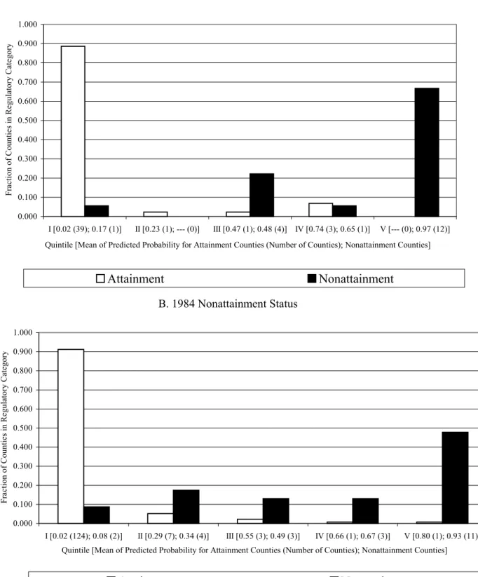
Before proceeding to the main matching results, Figure 4A displays the overlap in the distributions of the estimated propensity scores of the nonattainment and attainment counties based on Logit Specification 2. The figure contains the fraction and number of counties in each quintile, as well as the means of the propensity score by attainment status. The overlap is less than ideal here. For example, the highest quintile is entirely comprised of nonattainment counties and the mean propensity score among these counties is 0.97. Further, 39 of the 44 attainment counties are in the lowest quintile. It is evident that it will not be possible to find suitable matches for many of the nonattainment counties.
Returning to Table III B, the remaining panels present the results from tests of whether nonattainment status is associated with relative declines in SO2 concentrations in the post-treatment years.
Due to the difference in the regulation selection year SO2 concentrations across the matched counties, the
outcome is equal to the post treatment value of SO2 minus the value in the regulation selection year.
Again, separate results are reported for 1978, 1979, and 1980.
The results differ dramatically from the linear regression approach. They suggest that nonattainment status is associated with declines in SO2 pollution in this period. Logit Specification 1
indicates that by 1980, SO2 concentrations in 1978 SO2 nonattainment counties declined by roughly .003
ppm, while the specification 2 estimates indicate a decline that ranges from .003 ppm to .009 ppm. However, conventional criteria imply that all of the estimated declines are indistinguishable from zero in the 3rd post-period year. And, the small number of matched counties in Logit 2 limits the generality of the
findings. Nevertheless, the contrast between these estimated treatment effects and those from linear
matching process likely creates some positive dependence between them and this dependence is not accounted for.
regression is striking and underscores the poor reliability of linear regression when there is little overlap in the distributions of the covariates.20
B. 1981-1986
Tables IV A and IV B and Figure 4B are structured identically to Tables III A and III B and Figure 4A. The only difference with the analysis of the previous period is that the sample sizes are large enough to adjust for the lagged SO2 concentrations with a more flexible functional form. In particular,
the adjusted first difference estimates (in columns 2-5) and both of the logit specifications include quadratics and cubics of the lagged mean SO2 concentrations and quadratics of the extreme values
measures. Otherwise, the specifications are identical.
The results based on linear adjustment imply that nonattainment status is associated with modest reductions in SO2 concentrations. Almost the entire period decline has occurred in the first
post-treatment year. Interestingly, the estimates are roughly constant in columns (2) through (4).21 The estimates are also insensitive to the inclusion of a full set of state fixed effects as in column (5). Overall, the linear regression results suggest that nonattainment status is associated with a 6%-9% decline in SO2
concentrations by the end of the period. Again, none of the estimated parameters are statistically significant.
A few points emerge from the propensity score matching procedure. First, the matching almost completely eliminates the differences in regulation selection year SO2 concentrations. Second, there is
more overlap in the distribution of the propensity scores than in the 1975-80 period but there are still substantial differences in the two distributions. For example, 11 of the 12 counties in the highest quintile
20 There are at least two explanations for the differences between the estimated treatment effects from the
linear regression and propensity score approaches. First, the propensity score approach nonparametrically controls for observable variables while the linear regression is necessarily parametric. Second, the matching estimate is not based on the full set of nonattainment counties due to the poor overlap in the distributions of the propensity scores.
21 The parameter estimates and standard errors from the other covariates in the column (4) specification
when the dependent variable is the difference in the 1986 and 1983 SO2 concentrations are reported in
Appendix Table I. This table also reports this information for the analogous regression from the 1987-1992 period.
are nonattainment. Third, the treatment effects are smaller than the ones from linear regression and imply that nonattainment status had little effect on SO2 concentrations in this period.
C. 1987-1992
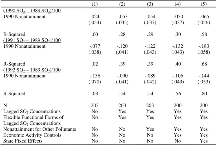
The 1987-92 period results are presented in Tables V A and V B and Figure 4C. The estimates based on linear adjustment suggest that nonattainment status is associated with a .0009 ppm to .0014 ppm reduction in SO2 pollution by the end of the period. These estimates would generally be considered
statistically different from zero. Interestingly, the largest estimate comes from the specification that includes state fixed effects when the estimate is identified from comparisons among nonattainment and attainment counties within the same state. These estimates suggest that 1990 nonattainment status reduced SO2 concentrations by 7%-11% in nonattainment counties by 1992.
Figure 4C demonstrates that the overlap of the distributions is better in this period than the other two. Although there are not any attainment counties in the two highest quintiles, 14 of the 19 nonattainment counties are in the lowest three quintiles where the entire attainment distribution is located. The estimated treatment effects are about half the magnitude of the linear regression treatment effects and are not statistically distinguishable from zero. This is likely driven by the inability to find suitable comparisons for the nonattainment counties with the highest probability of being designated nonattainment. Overall, the estimates from this period suggest that 1992 SO2 nonattainment status
modestly reduced SO2 concentrations in the post-period.
VII. Interpretation
The goal of the CAAAs is to bring all counties into compliance with the NAAQS. The EPA’s primary tool to achieve this goal is its ability to designate counties nonattainment and strictly regulate emitters in these areas. This paper has documented that by the late 1970s practically the entire U.S. had achieved the SO2 standard. Its most surprising finding is that a substantial number of counties with SO2
Through extensive conversations with EPA staff, I received a number of explanations for this seeming anomaly but none of them are completely satisfying.22 The most plausible explanation has two parts. First, it is the states’ responsibility to petition to get a county redesignated from nonattainment to attainment and this redesignation process is more difficult than might be expected. For example, this process frequently requires states to develop a local air pollution model that demonstrate that all areas within a county (not just the areas covered by the monitors) have SO2 concentrations below the federal
threshold. These models are often necessary even when all the local pollution monitors record concentrations that are below the federal standard. Importantly, these models are expensive to develop and states do not always have the necessary resources.
Second, the federal EPA staff suggested that they are receptive to requests to lessen the intensity of regulatory oversight in nonattainment counties that do not exceed the NAAQS. It may be easier to lessen the regulatory burden with these requests than by following all of the steps involved in obtaining a formal redesignation to attainment status.
Consequently, the stringency of regulations aimed at reducing a county’s SO2 pollution may
depend on a county’s nonattainment designation and whether its ambient SO2 concentration exceeds the
federal standards. If this is the case, this paper’s mixed results on the effectiveness of the SO2
nonattainment designation at reducing concentrations may not be surprising. However, it must be emphasized that this is a qualitative explanation of the results and cannot readily be subject to a rigorous test. Further, it does not explain why recent research has found that the TSPs and ozone nonattainment designations are associated with reductions in the ambient concentrations of these pollutants [6, 7, 16].
VIII. Conclusion
This study has used regulation categories specified by the Clean Air Act Amendments to empirically test whether this legislation contributed to the dramatic 80% decline in sulfur dioxide air
22 This section draws on conversations with Matthew Witosky of the EPA Region 6 office and a number
pollution that occurred over the last 30 years. Under this legislation, the EPA annually assigns every county a nonattainment or attainment designation. Stricter regulations apply in the nonattainment counties. Two primary findings are that the statutory selection rule that should have determined nonattainment status is not followed and that there are important observable differences between nonattainment and attainment counties. These findings make the evaluation problem especially difficult.
Linear regression and propensity score matching are used to control for the likely confounding caused by these differences. Notably, the matching appears to be especially useful when the observable differences between the nonattainment and attainment counties are greatest. The results indicate that SO2
nonattainment status is associated with modest reductions in SO2 air pollution, but a null hypothesis of
zero effect generally cannot be rejected. In summary, the paper finds that the SO2 nonattainment
designation played a minor role in the dramatic reduction of SO2 concentrations over the last three
decades.
The source of the dramatic reduction in ambient SO2 remains a mystery. The most likely
candidates are other features of the CAAAs or state and local regulations. In support of the latter possibility, there were large declines in SO2 concentrations that pre-dated the implementation of the 1970
CAAAs in a sample of 10 counties with monitors from 1969-1971. However, this extremely small sample may not be representative of the rest of the country. Overall, there is little evidence available to support or contradict alternative explanations.
References
[1] J. D. Angrist, Using social security data on military applicants to estimate the effect of military service earnings, Econometrica 66 (2), 249-288 (1998).
[2] J. D. Angrist and V. Lavy, Does teacher training affect pupil learning? Evidence from matched comparisons in jerusalem public schools, NBER Working Paper 6781 (1998).
[3] R. Becker and V. Henderson, Effects of air quality regulations on polluting industries, Journal of
Political Economy 108, 379-421 (2000).
[4] D. Card and D. Sullivan, Estimating the effect of subsidized training on movements in and out of employment, Econometrica 56 (3), 497-530 (1988).
[5] K. Chay, C. Dobkin, and M. Greenstone, Air quality, adult mortality, and the clean air act of 1970,
Journal of Risk and Uncertainty 27 (3), (2003).
[6] K. Chay and M. Greenstone, Does air quality matter? Evidence from the housing market, University
of Chicago Mimeograph (2000).
[7] K. Chay and M. Greenstone, Air quality, infant mortality, and the clean air act of 1970, University of
Chicago Mimeograph (2003a).
[8] K. Chay and M. Greenstone, The impact of air pollution on infant mortality: evidence from
geographic variation in pollution shocks induced by a recession, Quarterly Journal of Economics
118 (3), 1121-1167 (2003b).
[9] R. H. Dehejia and S. Wahba, Propensity score-matching methods for nonexperimental causal studies,
The Review of Economics and Statistics. 84 (1), 151-161 (2002).
[10] D. W. Dockery, et al., An association between air pollution and mortality in six u.s. cities, The New
England Journal of Medicine 329 (24), 1753-1759 (1993).
[11] I. M. Goklany, Clearing the Air: The Real Story of the War on Air Pollution, The Cato Institute, Washington, DC (1999).
[12] M. Greenstone, The impacts of environmental regulations on industrial activity: evidence from the 1970 and 1977 clean air act amendments and the census of manufacturers, Journal of Political
Economy 110 (6), 1175-1219 (2002).
[13] J. J. Heckman, H. Ichimura, and P. Todd, Matching as an econometric evaluation estimator, Review
of Economics Studies 65 (2), 261-294 (1998).
[14] J. J. Heckman, Micro data, heterogeneity, and the evaluation of public policy: nobel lecture,
Journal of Political Economy 109 (4), 673-748 (2001).
[15] J. J. Heckman and R. Robb, Alternative methods for evaluating the impact of interventions, in “Longitudinal Analysis of Labor Market Data, Econometric Society Monograph, No. 10” (J. J. Heckman and B. Singer, Eds.), Cambridge University Press, Cambridge, UK (1985).
[16] J. V. Henderson, Effects of air quality regulation, American Economic Review 86, 789-813 (1996). [17] L. B. Lave and G. S. Omenn, Clearing the Air: Reforming the Clean Air Act, The Brookings
Institution, Washington, DC (1981).
[18] R. A. Liroff, Reforming Air Pollution Regulations: The Toil and Trouble of EPA’s Bubble, The Conservation Foundation, Washington, DC (1986).
[19] M. R. Ransom and C. A. Pope III, External health costs of a steel mill, Contemporary Economic
Policy 8, 86-97 (1995).
[20] P. Rosenbaum and D. Rubin, The central role of the propensity score in observational studies for causal effects, Biometrika 70, 41-55 (1983).
[21] P. Rosenbaum and D. Rubin, Reducing bias in observational studies using subclassification on the propensity score, Journal of the American Statistical Association 79, 516-24 (1984).
[22] D. Rubin, Assignment to a treatment group on the basis of a covariate, Journal of Educational
Statistics 2 (1), 1-26 (1977).
[23] U.S. Environmental Protection Agency, Office of Air Quality Planning and Standards, National Air Pollutant Emission Trends, 1900-1994, U.S. Environmental Protection Agency: Research, Triangle Park, NC (1995).
[24] U.S. Environmental Protection Agency, The benefits and costs of the clean air act, 1970 to 1990,
Table I: Trends in EPA's SO2 Monitoring and Regulatory Programs, 1969-1997 Year Monitors Counties Population
(in millions) Annual Mean Annual Mean Mean of 2nd Monitored Total (Unweighted) (Pop. Weighted) Highest Daily Year 24 Hrs Year or 24 Hrs
(1) (2) (3) (4) (5) (6) (7) (8) (9) (10) (11) 1969 43 16 23.4 0.0380 0.0359 0.1904 8 8 9 --- ---1970 30 17 22.6 0.0301 0.0266 0.1493 6 8 8 --- ---1971 73 44 34.5 0.0224 0.0210 0.1121 9 14 18 --- ---1972 107 57 44.9 0.0206 0.0190 0.1009 6 14 15 --- ---1973 144 87 53.1 0.0185 0.0172 0.0970 12 17 20 --- ---1974 271 146 70.2 0.0172 0.0149 0.0833 11 20 25 --- ---1975 319 168 68.3 0.0150 0.0136 0.0746 10 21 23 --- ---1976 425 204 88.0 0.0143 0.0131 0.0728 11 22 23 --- ---1977 447 205 84.4 0.0142 0.0121 0.0758 10 22 25 --- ---1978 494 225 90.3 0.0127 0.0114 0.0646 2 13 13 41 87 1979 559 252 94.3 0.0125 0.0110 0.0682 3 12 14 43 84 1980 561 274 110.3 0.0105 0.0098 0.0540 1 15 15 45 83 1981 593 287 114.7 0.0098 0.0093 0.0558 1 8 8 47 80 1982 588 299 113.2 0.0093 0.0085 0.0479 0 6 6 42 60 1983 629 331 117.1 0.0089 0.0083 0.0461 1 4 4 36 53 1984 640 329 116.9 0.0094 0.0087 0.0521 2 6 7 31 48 1985 577 305 114.6 0.0088 0.0085 0.0474 0 6 6 34 51 1986 562 309 120.4 0.0084 0.0083 0.0449 0 3 3 36 49 1987 523 299 120.6 0.0076 0.0080 0.0388 1 4 4 29 48 1988 528 309 124.5 0.0079 0.0079 0.0413 1 3 4 30 49 1989 533 309 119.9 0.0078 0.0079 0.0392 0 1 1 30 49 1990 523 310 122.5 0.0072 0.0074 0.0363 1 1 2 29 46 1991 535 315 125.6 0.0070 0.0073 0.0363 0 2 2 28 46 1992 522 308 123.4 0.0064 0.0066 0.0338 0 1 1 25 46 1993 524 320 125.5 0.0061 0.0064 0.0314 0 2 2 --- ---1994 516 309 120.3 0.0059 0.0062 0.0331 0 1 1 --- ---1995 537 320 126.2 0.0048 0.0050 0.0255 0 0 0 --- ---1996 532 320 127.8 0.0048 0.0050 0.0265 0 1 1 --- ---1997 511 310 122.1 0.0048 0.0050 0.0250 0 1 1 ---
---Counties with Monitor Readings Exceeding Standard for:
SO2 Concentrations (ppm) SO2 Nonattainment Counties
Notes: The data sources are the EPA's SO2 monitoring network and the Code of Federal Regulations (CFR). The EPA considers a monitor "representative" of the prevailing ambient SO2 concentration if it records at least 6570 (out of a maximum of 8760) hourly concentrations in a year. The sample is restricted to monitors that meet this definition of representativeness in columns (1) - (9). Counties with at least 1 monitor satisfying this sample restriction form the universe of counties in column (7), but data from all monitors within those counties is used to determine whether the 24 hour SO2 air quality standard is exceeded. Column (10) reports the number of nonattainment counties in the entire U.S. Nonattainment status was published annually in the CFR beginning in 1978 and is unavailable before this year. The post-1992 data is currently unavailable in electronic form. The 1970 Census' population counts were used for the population measues from 1969 through 1975. The 1980 Census was used for 1976 through 1985 and the 1990 Census for 1986 through 1997. See the Data Appendix for more details.
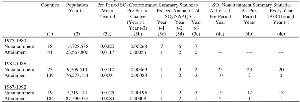
Table II: Pre-Period Characteristics of Counties, by Nonattainment Status
Counties Population Pre-Period SO2 Concentration Summary Statistics SO2 Nonattainment Summary Statistics
Year t-1 Mean Year t-1 Pre-Period Change Exceed Annual or 24 SO2 NAAQS At Least 1 Pre-Period All Pre-Period Every Year 1978 Through (Year t-1 – Year t-3) Year t-1 Year t-2 Year t-3
Year Years Year t-1
(1) (2) (3a) (3b) (3c) (3d) (3e) (4a) (4b) (4c)
1975-1980 Nonattainment 18 15,728,538 0.0220 -0.00268 7 6 7 --- --- --- Attainment 44 23,567,800 0.0117 0.00053 1 2 2 --- --- --- 1981-1986 Nonattainment 23 9,709,513 0.0110 -0.00369 1 3 2 23 23 20 Attainment 139 76,277,154 0.0091 -0.00083 1 2 3 10 2 2 1987-1992 Nonattainment 19 7,719,144 0.0125 -0.00196 1 2 3 19 17 13 Attainment 184 87,390,332 0.0084 0.00008 1 2 1 5 1 1
Note: Each panel reports summary information from the samples for each of the three 6 year periods analyzed in the paper. Column (1) reports the number of counties in the attainment and nonattainment categories in 1978, 1984, and 1990, respectively. Column (2) reports the population in each set of counties. Columns (3a) through (3e) report summary information on SO2 concentrations. Year t-1 refers to the regulation selection year, which is the year before the assignment of the nonattainment designation (i.e., 1977, 1983, and 1989). Years t-2 and t-3 are 2 and 3 years before the regulation selection year, respectively. Columns (4a) (4b), and (4c) report the number of counties designated nonattainment in any of the pre-period years (i.e., t-1, t-2, and t-3), each of the pre-period years, and in all years from 1978 through year t-1, respectively.
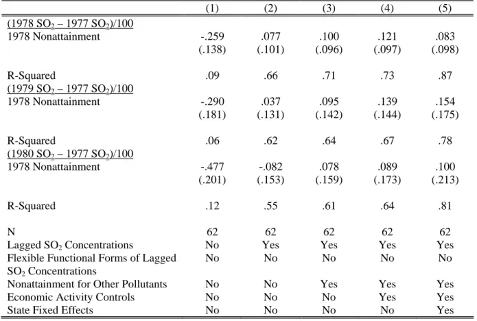
Table III: Estimated Effect of 1978 Nonattainment Status on Mean SO2 Concentrations
A. First Differences Estimates
(1) (2) (3) (4) (5) (1978 SO2 – 1977 SO2)/100 1978 Nonattainment -.259 .077 .100 .121 .083 (.138) (.101) (.096) (.097) (.098) R-Squared .09 .66 .71 .73 .87 (1979 SO2 – 1977 SO2)/100 1978 Nonattainment -.290 .037 .095 .139 .154 (.181) (.131) (.142) (.144) (.175) R-Squared .06 .62 .64 .67 .78 (1980 SO2 – 1977 SO2)/100 1978 Nonattainment -.477 -.082 .078 .089 .100 (.201) (.153) (.159) (.173) (.213) R-Squared .12 .55 .61 .64 .81 N 62 62 62 62 62
Lagged SO2Concentrations No Yes Yes Yes Yes
Flexible Functional Forms of Lagged SO2 Concentrations
No No No No No
Nonattainment for Other Pollutants No No Yes Yes Yes
Economic Activity Controls No No No Yes Yes
State Fixed Effects No No No No Yes
Notes: The entries are the parameter estimates from the 1978 nonattainment indicator variable and the associated standard errors from separate regressions. The standard errors are calculated with the Eicker-White formula to account for unspecified heteroskedasticity. See the text, particularly the description of equations (2) and (3), for further details. The included covariates are reported at the bottom of the table.
B. Propensity Score Matching Estimates
Logit Specification 1 Logit Specification 2
Caliper=.10 Caliper=.05 Caliper=.10 Caliper=.05
(1) (2) (1) (2) (1977 SO2)/100 1978 Nonattainment .402 .538 .314 .113 (.353) (.426) (.463) (.644) (1978 SO2 – 1977 SO2)/100 1978 Nonattainment .026 -.063 -.264 -.607 (.127) (.139) (.157) (.109) (1979 SO2 – 1977 SO2)/100 1978 Nonattainment -.070 -.102 -.213 -.711 (.183) (.183) (.239) (.209) (1980 SO2 – 1977 SO2)/100 1978 Nonattainment -.252 -.331 -.289 -.879 (.231) (.246) (.357) (.482)
# of 18 Treated that are Matched 11 8 6 3
# of 44 Controls that are Matched 44 43 4 2
Notes: The entries are the treatment effects and their standard errors from the propensity score matching procedure described in the text. Each nonattainment county is matched to all the attainment counties with propensity scores within the specified caliper. Logit Specification 1 includes the controls from the Column (2) specification of Table III A, plus the mean SO2 concentration in the regulation selection year. Logit Specification 2 includes
the controls from the Column (4) specification of Table III A, plus the mean SO2
Table IV: Estimated Effect of 1984 Nonattainment Status on Mean SO2 Concentrations
A. First Differences Estimates
(1) (2) (3) (4) (5) (1984 SO2 – 1983 SO2)/100 1984 Nonattainment .010 -.054 -.065 -.058 -.061 (.046) (.056) (.056) (.058) (.069) R-Squared .00 .12 .15 .17 .63 (1985 SO2 – 1983 SO2)/100 1984 Nonattainment .077 -.017 -.029 -.026 -.032 (.061) (.066) (.068) (.071) (.071) R-Squared .01 .22 .24 .25 .75 (1986 SO2 – 1983 SO2)/100 1984 Nonattainment -.025 -.098 -.078 -.085 -.069 (.053) (.057) (.060) (.061) (.070) R-Squared .00 .27 .28 .29 .65 N 162 162 162 159 159
Lagged SO2 Concentrations No Yes Yes Yes Yes
Flexible Functional Forms of Lagged SO2 Concentrations
No Yes Yes Yes Yes
Nonattainment for Other Pollutants No No Yes Yes Yes
Economic Activity Controls No No No Yes Yes
State Fixed Effects No No No No Yes
B. Propensity Score Matching Estimates
Logit Specification 1 Logit Specification 2
Caliper=.10 Caliper=.05 Caliper=.10 Caliper=.05
(1) (2) (1) (2) (1983 SO2)/100 1984 Nonattainment .100 .067 .071 .087 (.167) (.167) (.162) (.181) (1984 SO2 – 1983 SO2)/100 1984 Nonattainment -.006 .003 -.013 .003 (.072) (.074) (.072) (.076) (1985 SO2 – 1983 SO2)/100 1984 Nonattainment .041 .046 .028 .082 (.086) (.087) (.084) (.081) (1986 SO2 – 1983 SO2)/100 1984 Nonattainment -.022 -.023 -.038 .002 (.085) (.086) (.082) (.088)
# of 23 Treated that are Matched 16 15 16 14
# of 139 Controls that are Matched 139 116 136 124
Table V: Estimated Effect of 1990 Nonattainment Status on Mean SO2 Concentrations
A. First Differences Estimates
(1) (2) (3) (4) (5) (1990 SO2 – 1989 SO2)/100 1990 Nonattainment .024 -.053 -.054 -.050 -.065 (.054) (.035) (.037) (.037) (.056) R-Squared .00 .28 .29 .30 .58 (1991 SO2 – 1989 SO2)/100 1990 Nonattainment -.077 -.120 -.122 -.132 -.183 (.038) (.041) (.043) (.043) (.058) R-Squared .02 .39 .39 .40 .68 (1992 SO2 – 1989 SO2)/100 1990 Nonattainment -.136 -.090 -.089 -.106 -.144 (.070) (.041) (.042) (.043) (.053) R-Squared .03 .54 .54 .56 .80 N 203 203 203 200 200
Lagged SO2 Concentrations No Yes Yes Yes Yes
Flexible Functional Forms of Lagged SO2 Concentrations
No Yes Yes Yes Yes
Nonattainment for Other Pollutants No No Yes Yes Yes
Economic Activity Controls No No No Yes Yes
State Fixed Effects No No No No Yes
B. Propensity Score Matching Estimates
Logit Specification 1 Logit Specification 2
Caliper=.10 Caliper=.05 Caliper=.10 Caliper=.05
(1) (2) (1) (2) (1989 SO2)1/100 1990 Nonattainment .050 .013 .119 .121 (.151) (.152) (.162) (.160) (1990 SO2 – 1989 SO2)1/100 1990 Nonattainment .001 .001 .001 -.002 (.042) (.042) (.046) (.046) (1991 SO2 – 1989 SO2)1/100 1990 Nonattainment -.034 -.033 -.038 -.036 (.056) (.055) (.061) (.062) (1992 SO2 – 1989 SO2)1/100 1990 Nonattainment -.053 -.047 -.065 -.067 (.064) (.064) (.070) (.071)
# of 19 Treated that are Matched 15 15 14 14
# of 184 Controls that are Matched 184 183 181 181