Antarctic clouds, supercooled liquid water and mixed phase, investigated with DARDAR: geographical and seasonal variations

HAL Id: insu-02136183

https://hal-insu.archives-ouvertes.fr/insu-02136183

Submitted on 21 May 2019

HAL is a multi-disciplinary open access

archive for the deposit and dissemination of

sci-entific research documents, whether they are

pub-lished or not. The documents may come from

teaching and research institutions in France or

abroad, or from public or private research centers.

L’archive ouverte pluridisciplinaire HAL, est

destinée au dépôt et à la diffusion de documents

scientifiques de niveau recherche, publiés ou non,

émanant des établissements d’enseignement et de

recherche français ou étrangers, des laboratoires

publics ou privés.

phase, investigated with DARDAR: geographical and

seasonal variations

Constantino Listowski, Julien Delanoë, Amélie Kirchgaessner, Tom

Lachlan-Cope, John King

To cite this version:

Constantino Listowski, Julien Delanoë, Amélie Kirchgaessner, Tom Lachlan-Cope, John King.

Antarc-tic clouds, supercooled liquid water and mixed phase, investigated with DARDAR: geographical and

seasonal variations. Atmospheric Chemistry and Physics, European Geosciences Union, 2019, 19 (10),

pp.6771-6808. �10.5194/acp-19-6771-2019�. �insu-02136183�

Atmos. Chem. Phys., 19, 6771–6808, 2019 https://doi.org/10.5194/acp-19-6771-2019 © Author(s) 2019. This work is distributed under the Creative Commons Attribution 4.0 License.

Antarctic clouds, supercooled liquid water and mixed phase,

investigated with DARDAR: geographical and seasonal variations

1_{LATMOS/IPSL, UVSQ Université Paris-Saclay, UPMC Univ. Paris 06 Sorbonne Universités, CNRS, Guyancourt, France} 2_{British Antarctic Survey, Natural Environment Research Council, High Cross, Madingley Road,}

Cambridge, CB3 OET, UK

Correspondence: Constantino Listowski (constantino.listowski@latmos.ipsl.fr) Received: 22 November 2018 – Discussion started: 17 December 2018

Revised: 13 March 2019 – Accepted: 18 April 2019 – Published: 21 May 2019

Abstract. Antarctic tropospheric clouds are investigated us-ing the DARDAR (raDAR/liDAR)-MASK products between 60 and 82◦S. The cloud fraction (occurrence frequency) is divided into the supercooled liquid-water-containing cloud (SLC) fraction and its complementary part called the all-ice cloud fraction. A further distinction is made between SLC involving ice (mixed-phase clouds, MPC) or not (USLC, for unglaciated SLC). The low-level (< 3 km above surface level) SLC fraction is larger over seas (20 %–60 %), where it varies according to sea ice fraction, than over continental regions (0 %–35 %). The total SLC fraction is much larger over West Antarctica (10 %–40 %) than it is over the Antarc-tic Plateau (0 %–10 %). In East AntarcAntarc-tica the total SLC fraction – in summer for instance – decreases sharply pole-wards with increasing surface height (decreasing tempera-tures) from 40 % at the coast to < 5% at 82◦S on the plateau. The geographical distribution of the continental total all-ice fraction is shaped by the interaction of the main low-pressure systems surrounding the continent and the orography, with little association with the sea ice fraction. Opportunistic com-parisons with published ground-based supercooled liquid-water observations at the South Pole in 2009 are made with our SLC fractions at 82◦S in terms of seasonal variability, showing good agreement. We demonstrate that the largest impact of sea ice on the low-level SLC fraction (and mostly through the MPC) occurs in autumn and winter (22 % and 18 % absolute decrease in the fraction between open water and sea ice-covered regions, respectively), while it is almost null in summer and intermediate in spring (11 %). Monthly variability of the MPC fraction over seas shows a maximum at the end of summer and a minimum in winter. Conversely,

the USLC fraction has a maximum at the beginning of sum-mer. However, monthly evolutions of MPC and USLC frac-tions do not differ on the continent. This suggests a seasonal-ity in the glaciation process in marine liquid-bearing clouds. From the literature, we identify the pattern of the monthly evolution of the MPC fraction as being similar to that of the aerosols in coastal regions, which is related to marine bio-logical activity. Marine bioaerosols are known to be efficient ice-nucleating particles (INPs). The emission of these INPs into the atmosphere from open waters would add to the tem-perature and sea ice fraction seasonalities as factors explain-ing the MPC fraction monthly evolution.

1 Introduction

Antarctic clouds need to be correctly represented in regional and global atmospheric models to improve daily operational forecast as well as future global climate predictions. Clouds’ contribution to Antarctica’s ice mass balance via precipita-tion and to the Antarctic surface energy budget are poorly constrained. However, it has been shown that they exert a warming effect on the ice sheet (Scott et al., 2017; Nicolas et al., 2017). The microphysical properties of clouds can also affect circulation at much lower latitudes due to the changes they induce in the energy budget and the meridional temper-ature gradients (Lubin et al., 1998). In the Southern Ocean (SO) and Antarctic seas, clouds cause major radiative biases in climate prediction models (Haynes et al., 2011; Flato et al., 2013; Bodas-Salcedo et al., 2014; Hyder et al., 2018). The

supercooled liquid water causes major difficulties in cloud microphysics modelling over the SO (Bodas-Salcedo et al., 2016). It is difficult to conceive that the SO energy budget’s long-standing dilemma can be solved without paying close attention to clouds in the Antarctic region (60–90◦S), which is the southern boundary of the SO and more generally the cold sink of our planet. In Antarctica, surface radiation bi-ases of several tens of watt per square metre are derived from mesoscale high-resolution models, which point to ma-jor problems in the simulation of the cloud cover (Bromwich et al., 2013a) and of the cloud thermodynamic phase and more particularly of the supercooled liquid water (the water staying in the liquid phase below the freezing point) (Law-son and Gettelman, 2014; King et al., 2015; Listowski and Lachlan-Cope, 2017). Ultimately, the right balance of ice vs. liquid mass in Antarctic clouds in high-resolution models will largely depend on the way the ice microphysics is imple-mented, the way it leaves or removes the formed supercooled liquid water (Listowski and Lachlan-Cope, 2017), and how processes like secondary ice multiplication observed in that region (Grosvenor et al., 2012; Lachlan-Cope et al., 2016; O’Shea et al., 2017) can be correctly accounted for (Young et al., 2019). This balance will in turn determine the ability of the model to minimise the surface radiative biases. Im-proving the modelling of the supercooled liquid water over the region may induce drastic changes in the simulations of clouds in the SO (Lawson and Gettelman, 2014), without being certain that any improvement for one part of the re-gion will also lead to the improvement of cloud modelling over the rest of the Antarctic. Hence, being able to track the Antarctic-wide formation of supercooled liquid and the mixed phase and adding to the efforts of ground-based obser-vation studies (Lawson and Gettelman, 2014; Scott and Lu-bin, 2014; VanTricht et al., 2014; Gorodetskaya et al., 2015; Silber et al., 2018) appear to be necessary steps towards improve cloud microphysics modelling in the Antarctic for lowering the surface radiative biases across the regions that are observed in the climate prediction models (e.g. Lenaerts et al., 2017).

Because of the remoteness of the continent, the harsh en-vironment to which every ground or aircraft operation is exposed, and the inaccessibility of most of Antarctica to in situ observations, satellite observations appear as a wel-come if not crucial complement. For instance, Palerme et al. (2014) used satellite radar products to build the first cli-matology of snowfall rates across the Antarctic continent (updated by Palerme et al., 2019). Nonetheless, a few air-borne and ground-based campaigns took place in the last 10 years, presenting new cloud and precipitation studies that un-veiled cloud or precipitation properties in different regions like the Antarctic Peninsula (Grosvenor et al., 2012; Lachlan-Cope et al., 2016), the Weddell Sea (O’Shea et al., 2017), the West Antarctic Ice Sheet (Scott and Lubin, 2014; Silber et al., 2018), Adélie Land (Grazioli et al., 2017a, b; Gen-thon et al., 2018), Dronning Maud Land (Gorodetskaya et al.,

2015) or the South Pole (Lawson and Gettelman, 2014). In order to get the needed wider perspective on the Antarctic-wide geographical distribution and seasonal variation in the cloud thermodynamic phase and the supercooled liquid wa-ter, we make use of the synergetic DARDAR (raDAR/liDAR) products (Delanoë and Hogan, 2010; Ceccaldi et al., 2013), which were recently used for mapping the Arctic mixed-phase clouds (Mioche et al., 2015). Bromwich et al. (2012), who gave a review on all aspects of tropospheric Antarctic clouds, illustrated the strength of using active remote sens-ing over passive remote-senssens-ing systems to correctly capture cloud cover over icy terrain and especially over the Antarc-tic continent. Previous studies used other radar–lidar satellite products to describe the horizontal and vertical distribution of clouds in the SO and the Antarctic during the 2007–2009 period (Verlinden et al., 2011), the ice microphysical prop-erties and the cloud distribution in the Antarctic during the 2007–2010 period (Adhikari et al., 2012). Jolly et al. (2018) described the cloud and phase distribution over the Ross Sea and the Ross Ice Shelf (RIS) according to a classification of dynamical regimes evidenced in previous works. However, it is the first time that the DARDAR products are used in that region. More particularly, we aim to describe the Antarctic-wide cloud geographical and seasonal variation on a monthly to seasonal scale with a specific focus on the supercooled liq-uid water (SLW).

In Sect. 2 we recall the main features of the Antarctic at-mosphere, and in Sect. 3 we present the data and the method we use. In Sect. 4 we present results on the seasonal, geo-graphical and vertical variations of different cloud types, as well as the monthly variations over specific regions. We also present comparisons made with ground-based measurements taken over our period of interest. Finally, we investigate links with the sea ice fraction for the different cloud phases. In Sect. 5, we discuss the results and, importantly, the link be-tween the seasonality of mixed-phase clouds and the sea ice fraction and provide an explanation of the observed monthly time series for these clouds. Section 6 concludes and recalls our main results.

2 The Antarctic environment

We recall the salient features of the Antarctic environment, focusing on our 4 years of interest (2007–2010; see Sect. 3). Antarctica is characterised by a very contrasted topography illustrated in Fig. 1. Recall that “Antarctica” refers to the con-tinent while “Antarctic” refers to the whole region, includ-ing the ocean (60–82◦S in this study). West Antarctica (WA) has the lowest average surface height, with a peak altitude at around 2.5 km above sea level (a.s.l.) in the interior of the West Antarctic Ice Sheet (WAIS). East Antarctica (EA) hosts the Antarctic Plateau, which reaches altitudes of 4 km a.s.l.

Antarctica is surrounded by an uninterrupted stream of westerlies favoured by the lack of land as illustrated by

C. Listowski et al.: Antarctic clouds, supercooled liquid water and mixed phase 6773

Figure 1. The Antarctic continent (Antarctica) and its topography (Fretwell et al., 2013), along with names of places mentioned in this study. The Transantarctic (TA) Mountains separate West Antarc-tica (WA) from East AntarcAntarc-tica (EA). Two ice shelves are also re-ported: the Ross Ice Shelf (RIS) and the Amery Ice Shelf (AIS). MBL stands for Marie Byrd Land and PEL for Princess Elisabeth Land. Bellings. refers to Bellingshausen. The location of two UK, one French–Italian and one US Antarctic stations are indicated with markers: Rothera (triangle), Halley VI (circle), Concordia (square) and Amundsen–Scott South Pole Station (diamond shape). Mea-surements made at these stations are used in Sect. 4.4.

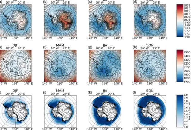
the isobars of the mean sea level pressure (MSLP) depicted in Fig. 2a. We used ERA-Interim reanalysis monthly aver-age products (Dee et al., 2011) averaver-aged over 2007–2010 for each season. There are three permanent (climatic) low-pressure systems (King and Turner, 1997), with average posi-tions that are essentially determined by the topography of the continent (Baines and Fraedrich, 1989). The most obvious of these lows is the Amundsen Sea low (ASL) to the west of the continent, across the Amundsen and the Ross seas around 140◦W (Fig. 2a–d). The two other lows are located around 100◦E (see in Fig. 2b and c) and around 30◦E (see in Fig. 2a and c).

Along the coastline an easterly circulation prevails, fuelled by the above-mentioned lows and also by the regime of kata-batic winds, which characterise Antarctica (see e.g. King and Turner, 1997). These downslope winds are induced by the strong cooling of the atmosphere over the high-altitude icy terrain in the interior of the continent, and their deviation to the west while reaching the coast – due to the Coriolis force – contributes to the coastal easterly circulation. Hence, a weak anticyclonic regime prevails in the interior of the continent in EA, where air subsidence contributes to the outward surface

flow of the katabatic wind regimes (James, 1989). A cyclonic circulation dominates above the surface with a strong perma-nent low above the RIS area, as illustrated by the 500 hPa geopotential height contour lines plotted in Fig. 2e–h.

Finally, the sea ice exerts control over the moisture and heat transported into the lower atmosphere and therefore will affect the cloud cover and their properties, as evidenced in the Arctic (Kay and Gettelman, 2009; Taylor et al., 2015; Morri-son et al., 2018) and over the Southern Ocean in winter (Wall et al., 2017), spring and summer (Frey et al., 2018). The sea ice can also impact cloud formation by acting as a source of cloud condensation nuclei (for sea salt coming from blowing snow; see e.g. Yang et al., 2008; Legrand et al., 2016), al-though this link between sea ice and clouds has been much less investigated in the literature so far. Figure 2i–l show the average seasonal sea ice fraction over 2007–2010 plotted us-ing the passive microwave sea ice concentration data record (Cavalieri et al., 1996) archived by the National Snow and Ice Data Center (NSIDC) and projected onto the grid used to map the cloud fraction (see Sect. 3.2). The largest extent of sea ice occurs in September and the smallest in February. The westernmost part of the Weddell Sea shows a persistent and dense sea ice coverage throughout the year.

3 Data and method

3.1 The DARDAR-MASK version 2 products

The DARDAR products were developed in order to use the complementarity of the CALIOP (Cloud Aerosol Lidar with Orthogonal Polarization) lidar on board CALIPSO (Cloud Aerosol Lidar and Infrared Pathfinder Satellite Observations, Winker et al., 2010) and the Cloud Profiling Radar (CPR) on board CloudSat (Stephens et al., 2002). Both satellites are part of the A-Train constellation (Stephens et al., 2002). A seamless retrieval algorithm uses both signals to obtain two products, namely the DARDAR-MASK (Delanoë and Hogan, 2010; Ceccaldi et al., 2013) and the DARDAR-CLOUD (Delanoë and Hogan, 2008; Cazenave et al., 2018). Due to their different wavelengths, the radar and the lidar are not sensitive to the same part of the hydrometeor size distribution. The cloud radar will be more sensitive to the large particles and will miss very small droplets or ice crys-tals. In contrast the lidar is very sensitive to the concentra-tion of hydrometeors and can detect optically thin cirrus and supercooled water but suffers from a strong attenuation ef-fect. The lidar signal is almost fully extinguished in a cloud with an optical thickness larger than 3. This synergy pro-vides the unique opportunity to vertically describe the inte-rior of clouds across the entire Antarctic. In this study we only make use of the DARDAR-MASK product, which con-tains information on the three-dimensional cloud thermody-namic phase classification at the vertical resolution of the li-dar (60 m) and at the horizontal resolution of the CPR 1.7 km

Figure 2. Four-year (2007–2010) seasonal averages of (a–d) the mean sea level pressure (MSLP, in hPa), (e–h) the 500 hPa geopotential height (m). Panels (i–l) show the 4-year seasonal average of the sea ice fraction obtained from the National Snow and Ice Data Center and projected onto the grid used to map the cloud fraction (see Sect. 3.2). The topography contours are also indicated.

(along track) ×1.4 km (cross track). We use the most recent version 2 of those products recently made available by the Aeris/ICARE data centre and that are introduced in Ceccaldi et al. (2013). The DARDAR-MASK v2 is built from the li-dar attenuated backscatter coefficient at 532 nm (CALIPSO Level 1 products, version 4-1), the vertical feature mask (VFM, CALIPSO Level 2 products, version 4-1) and the 94 GHz radar reflectivity (CloudSat 2B GEOPROF, version 4). The ECMWF-AUX (version R04) products provide ther-modynamic state variables stored in the DARDAR-MASK. They are analysis products provided by the European Cen-tre for Medium-Range Weather Forecasts (ECMWF) that are interpolated on the CloudSat grid by the CloudSat team. The DARDAR-CLOUD products, which give access to the ice microphysical properties like the ice water content and the ice effective radius, will be investigated in a separate work (their version 2 products were not yet available at the time of writing).

Substantial improvements were made for the DARDAR-MASK v2 in comparison to v1 (Ceccaldi et al., 2013). The main features are a better assessment of the higher cloud cover (above 5 km height), which was overestimated in v1 due to a block effect present in the CALIOP VFM (An over-counting of cloud occurrences due to a coarser resolution of the VFM projected on the DARDAR 60 m vertical resolution

grid). As version 2 now relies directly on the original 60 m resolution lidar signal, it does not suffer from this effect. The other significant improvement is a better categorisation of su-percooled water pixels that were overestimated in v1 in the lowest atmospheric layers (Ceccaldi et al., 2013). Two ex-amples of typical Antarctic DARDAR scenes are shown in Fig. 3. The topography shows up as brown in the colour-coded DARDAR-MASK transects. These two examples of transects illustrate the different categories of the mask in-troduced in Ceccaldi et al. (2013), along with some com-mon features of the cloud phase and its vertical distribu-tion observed in the Antarctic region. The summer transect (top) shows the high occurrences of supercooled liquid wa-ter (SLW) with (light green) or without (red) ice, allowing differentiation between mixed-phase and unglaciated layers. The early spring transect (bottom) is an example of intru-sion of large synoptic-scale systems that can happen over the Antarctic plateau, to the east of the continent, with no or very few occurrences of a mixed phase.

As we are interested in mapping the occurrences of the liquid and the ice phase, we do not use the distinct cate-gories developed for the ice phase but we consider all the ice categories together (namely the ice clouds, the highly con-centrated ice and the spherical or 2-D ice). Hence we track the general ice phase occurrences (light blue, dark blue,

pur-C. Listowski et al.: Antarctic clouds, supercooled liquid water and mixed phase 6775

Figure 3. Two examples of DARDAR-MASK transects (altitude vs. latitude and longitude) illustrating the various categorisation included in the DARDAR-MASK version 2. The summer transect (a) occurred on 3 February 2007, while the early spring one (b) occurred on 11 September 2009. The small map next to each transect shows the satellite track (solid red line) projected over the Antarctic region. The circle indicates the beginning of the tracks across the Antarctic.

ple of the colour-coded mask) and the occurrences of SLW wether it is mixed with ice (light green of the colour-coded mask) or not (red of the colour-coded mask). The vast ma-jority of Antarctic tropospheric clouds occurs in these cate-gories. Warm liquid cloud occurrence is observed on the mar-gins of the domain (60–62◦S; 100–180◦W) in very negligi-ble amounts compared to the rest of the investigated cloud phases.

Finally, note that the category “multiple scattering due to SLW” was not introduced in Ceccaldi et al. (2013) and was subsequently added by Ceccaldi (2014, their Sect. III.3.5). As explained in that work, this corresponds to the detection of a backscatter signal from below the SLW layer, which is still important despite a strong attenuation of the lidar signal there. If the radar does not detect any ice, this signal has to be caused by the multiple scattering in the layer of supercooled droplets above.

3.2 Methodology 3.2.1 Statistics

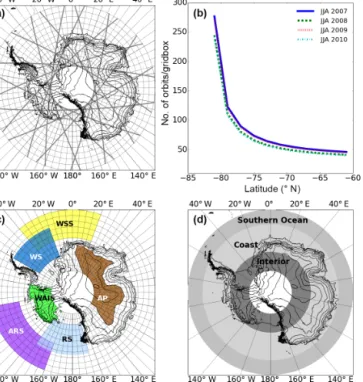
About 15 overpasses occur each day over the Antarctic re-gion (Fig. 4a), which we define as the rere-gion poleward of 60◦S. Following Adhikari et al. (2012) and Mioche et al. (2015), we divide the area into grid boxes of 2◦in latitude

and 5◦ in longitude, which correspond approximately to a grid box of 280 km by 220 km at 60◦S and of 280 km by 80 km at 82◦S (the southernmost latitude observed by the satellites). The grid, on which the overpasses are combined to derive the occurrence frequency of the clouds, appears in the maps of Fig. 4a and c. The shaded areas in Fig. 4d de-limit the investigated Antarctic region in this study located between 60 and 82◦S and the three different latitudinal bands used to derived latitudinally averaged vertical transects: the Southern Ocean (SO) transect (60–65◦S), the coastal tran-sect (65–75◦S) and the interior transect (75–82◦S).

The sun-synchronous polar orbit of the satellites results in an exponentially increased sampling of the continent as we observe closer to the pole (Fig. 4b). The SO limit at 60◦S shows one overpass every 2 days (∼ 45 per season) per grid box, while the southernmost limit at 82◦S shows on average more than 2.5 overpasses per day (∼ 250 per season) per grid box. The sharp increase in the statistics towards the South Pole is welcome as it is the area where the cloud cover is the lowest (e.g. Bromwich et al., 2012). The measurement statis-tics hardly change along a given parallel due to the symmetry of the polar orbiters’ trajectories in relation to the South Pole (hence the zonal average presented in Fig. 4b). The measure-ment statistics are very similar from one season and one year to the next. JJA is shown as an example in Fig. 4b. Only DJF 2010 shows a significant reduction (by 40 %) in the number

Figure 4. (a) The Cloudsat tracks across the Antarctic on 1 Jan-uary 2007, and the grid (grid boxes of 2◦in latitude and 5◦in lon-gitude) used to derive the geographical distribution of cloud occur-rences and extending between 60 and 82◦S (b) The zonally aver-aged number of satellite overpasses per grid box as a function of latitude, for the whole winter season each year. (c) Areas of inter-est used in the study and introduced in Sect. 4.3 to invinter-estigate the monthly evolution of cloud occurrences. They are called WSS (in the Weddell Sea sector), ARS (in the Amundsen–Ross sector), WS (in the Weddell Sea), RS (in the Ross Sea), the WAIS (on the West Antarctic Ice Sheet) and AP (on the Antarctic Plateau). Names are recalled in Table 1. (d) The three latitudinal bands used for the av-erage vertical transects presented in Sect. 4.2.

of available DARDAR products. We use the 4 years 2007– 2010 as they are the only 4 full years with night-time obser-vations for the CPR, which works only by daylight due to a battery failure from 2011 onwards.

Note that despite the different times of satellite overpasses over the different Antarctic areas, we do not expect any di-urnal cycle to bias our observations and conclusions. For in-stance, the local (UTC) times of the overpasses above the grid box including Rothera are 02:00 (05:00) and 17:00 (20:00), while for Halley they are on average at 01:30 (01:30) and 18:00 (18:00). The morning and evening times corre-spond to the descending and ascending nodes of the satellite overpasses. Cloud cover varies diurnally as a result of the development of convection, but in and around Antarctica this will be weak at all times of the year. Over the ocean, diur-nal variation in the surface temperature is small. Even over the ice sheets, diurnally varying convective boundary layers develop in summer at locations like Dome C, but these lay-ers are very shallow and do not generate convective cloud

(King et al., 2006). Moreover, the ceilometer data introduced in Sect. 3.3 and used in Sect. 4.4.1 confirm the low amplitude of the cloud occurrence diurnal cycle (not shown) at Halley (2.5 % absolute variation) and Rothera (6 % absolute varia-tion) compared to the average amplitude of the seasonal cy-cle (> 20 %).

3.2.2 Cloud fraction mapping

Following Mioche et al. (2015) in their study of Arctic clouds with DARDAR v1 products, we derive a (temporal abso-lute) cloud fraction (or cloud occurrence frequency) Fcloud.

It is the ratio of the number of cloud occurrences Ncloud

per grid box over the number of observations (footprints) Nfootprintsin that grid box: Fcloud=Ncloud/Nfootprints. A valid

cloud occurrence is an occurrence of at least three adjacent vertical pixels flagged with the same condensed phase. We do not distinguish between precipitable and non-precipitable frozen hydrometeors as the ice phase includes both cloud ice and snow in the DARDAR products. We focus on tro-pospheric clouds, so that stratospheric features are not ac-counted for in the derived horizontal or vertical distributions of the cloud fraction. We use the tropopause height provided by the CALIOP product and stored in the DARDAR product. The tropopause lies at ∼ 9 km in the summer and at ∼ 12 km in the winter. The same method is used to derive the fraction FXof any given cloud type X (see below). This technique is

applied for every month to derive a monthly averaged frac-tion in every single lat–lon grid box. To obtain the cloud (or any cloud type) seasonal fraction, the number of total occur-rences of clouds (or any cloud type) over the 3 months of interest is divided by the total number of footprints in each grid box over these months. The relative fraction (as opposed to the previously defined absolute fraction) can also be com-puted for the different cloud types, where the number of ob-servations Nfootprintsis replaced by the number of cloud

oc-currences Ncloud in the ratio. In DJF (austral summer) of a

given year, the month of December is the one from the previ-ous year. For instance, DJF 2007 uses December 2006. Thus, we obtain maps of the geographical distribution of the cloud fractions. The vertical distribution of the cloud or any cloud type fraction is also computed by deriving the ratios as ex-plained above but for each of the 60 m vertical pixels.

The fraction of SLW-containing clouds is called the SLC fraction, FSLC. Table 1 recalls the acronyms used for the

var-ious cloud types (as well as the ones for specific Antarctic regions). The DARDAR-MASK includes a mixed-phase cat-egory (“SLW with ice” – first type), and we extend this cate-gory by adding the clouds where a pure SLW layer is detected with at least three adjacent vertical pixels containing ice be-low (second type), folbe-lowing Mioche et al. (2015). In prac-tice, most of the detected mixed-phase clouds are of the first type, but pure SLW layers with an ice phase immediately be-low are clearly detected. We interpret these as occurrences of a mixed phase since the ice below is immediately in contact

C. Listowski et al.: Antarctic clouds, supercooled liquid water and mixed phase 6777

with the liquid layer; their microphysics must be interacting. Note that cloud where ice crystals are too small and/or too few to be detected by the radar in the top SLW layer of the cloud is also possible (recall that in the upper atmosphere, for instance, the CPR cannot detect thin cirrus). A cloud top made out of SLW with ice precipitating below is characteris-tic of boundary layer mixed-phase clouds (e.g. Korolev et al., 2017) and, in practice, cloud layers flagged by DARDAR as actual mixed phase (and not pure SLW) come systematically along with ice below. The mixed-phase clouds (first and sec-ond types) are described by the MPC fraction, FMPC.

Su-percooled liquid-water-containing clouds (SLCs) that are not part of any mixed-phase clouds as defined above (hence be-ing pure liquid) are categorised as unglaciated supercooled liquid clouds (USLCs), with a fraction of FUSLC. They are

liquid clouds for which no glaciation process has occurred (see for example Fig. 3a: the layer appearing in red around 2 km altitude at longitudes between 51◦_{W and 82}◦_{W). By}

“glaciation processes” we designate the processes by which a pure liquid layer becomes a mixed-phase layer. The SLC fraction will refer to any detection of SLW (whether involved in a mixed layer or not). Adding the USLC fraction and the MPC fraction gives the SLC fraction. An all-ice cloud cate-gory is defined and accounts for occurrences of the ice phase when no SLW at all is present in the investigated part of the troposphere (the whole of it or the low, middle or high part of it). This is proven to be useful to investigate occurrences of strict ice-only processes in order to put the behaviour of these clouds into perspective with SLCs. Importantly, all-ice and SLC fractions are complementary by definition. We can summarise all the fractions we are interested in and their re-lationships by writing the following:

Fcloud=Fall-ice+FSLC (1)

FSLC=FMPC+FUSLC. (2)

Following Mioche et al. (2015), a distinction is made be-tween low-level clouds (at altitudes bebe-tween 500 m and 3 km above ground level), mid-level clouds (3–6 km above ground level) and high-level clouds (more than 6 km above ground level). When no restriction to a particular altitude level is considered, we will speak about the total cloud fraction or, simply, the cloud fraction. We choose to use ground level and not mean sea level as a reference for altitudes and, similarly, altitude levels rather than pressure levels in order to remain consistent in our description of clouds across the Antarc-tic region, where ground levels between 0 and 4 km above mean sea level are found. Using a mean sea level reference or pressure levels to discriminate between clouds of differ-ent height would artificially lead to an empty low-level cloud category as looking closer to the pole. Thus we do not make use of the International Satellite Cloud Climatology Project (ISCCP, Rossow and Schiffer, 1999) pressure levels (680 and 440 hPa, which approximately correspond to 3 and 6 km

Table 1. Acronyms used in the text to designate some cloud phase or cloud types and some Antarctic places or areas.

SLW Supercooled liquid water SLCa SLW-containing cloud MPCa Mixed-phase cloud USLCa Unglaciated SLW cloud WA West Antarctica EA East Antarctica SO Southern Ocean WSSb Weddell Sea sector ARSb Amundsen–Ross sector WSb Weddell Sea

RSb Ross Sea

WAISb West Antarctic Ice Sheet APb Antarctic Plateau AIS Amery Ice Shelf RIS Ross Ice Shelf

a_{Their fractions are linked by Eq. (2).} b_{Geographical areas are defined in Fig. 4c and}

their names relate to the regions in which they are located.

above mean sea level) as this was done for studies over the SO only. Our goal is to describe the marine and continen-tal clouds of the Antarctic and their differences rather than comparing our observations to the numerous characterisa-tions made over part of or the whole of the SO using A-Train (and sometimes DARDAR v1) and/or ISCCP observations (e.g. Hu et al., 2010; Haynes et al., 2011; Huang et al., 2012; Mason et al., 2014; Bodas-Salcedo et al., 2014; Huang et al., 2015).

3.2.3 Limitations of the products

Finally, two main limitations have to be considered when us-ing space-borne lidar and radar data sets. First, the strong extinction of the lidar meeting a supercooled liquid layer pre-vents it from detecting any other liquid layer that could ex-ist below this one. The lidar signal can also be extinguished closer to the surface because of optically thick ice clouds above. Figure 3a shows grey-shaded areas flagged “presence of liquid unknown”. This is illustrative of the lidar signal extinction below the detections of supercooled liquid layers (first part of the transect in Fig. 3a). This category is flagged in the mask when the lidar signal is extinguished and when at the same time the radar does not detect any ice. Second, the surface clutter or blind zone of the radar (Tanelli et al., 2008) (surface wave reflection blurring the signal) prevents it from detecting any ice cloud (or identifying the ice part of the MPC) close to the surface. This can be clearly seen when the identification of the ice phase ceases when nearing the ground (at ∼ 500 m above the surface) in Fig. 3a after the longitude 168◦E and in Fig. 3b right at the beginning of the transect.

Practically, the clutter height is not constant, and it is flagged in the CloudSat products used to build the DARDAR-MASK products so that the latter does not take into ac-count the radar signal in areas where the clutter is identi-fied. This will result effectively in a reduced statistics close to the surface. The lidar information, however, is not filtered out. Hence, detection of supercooled liquid layers even in the blind zone of the radar can happen. To derive the geo-graphical distribution of the cloud fraction we consider the atmosphere above 500 m above the surface, ignoring a large part of the radar signal ground contamination in order not to work with the very reduced radar or lidar statistics too close to the surface, following (Mioche et al., 2015). Their statis-tics was approximately halved (∼ 60 % loss) between 500 and 1000 m above the surface. In Appendix A we show ver-tical transects of the occurrence frequency of the lidar extinc-tions and the radar signal contamination (Fig. A1). Addition-ally, the monthly time series of the occurrences of radar sig-nal contamination and lidar extinction or attenuation above 500 m above the surface are shown in Fig. A2. In our data set, ∼ 80 % of the radar observations are still available at an altitude of 500 m above the ground (Fig. A2a), and almost no contamination occurs above 1 km. Importantly, there is almost no seasonality in the radar clutter occurrences. Sea-sonality in the radar signal reflection can occur because of the changing nature of the surface (caused by more waves at the sea surface at a given time of the year Tanelli et al., 2008). The statistics of lidar observations show a ∼ 55 % occurrence in the signal extinction at 1 km above the surface and ∼ 65 % at 500 m above the surface (Fig. A2b). The lower altitude cut-off set at 500 m above the surface to derive the geographical distributions of the cloud fractions does not affect our conclu-sions, and this is discussed in Appendix B. It is mainly the absolute value of the USLC monthly fraction that is affected by this cut-off but not its relative variations (Fig. B1). 3.3 Ceilometer data set

Vaisala CT25k ceilometers were installed at Halley and Rothera in 2003, their purpose being to support logistical and scientific aircraft operations. They operate on the li-dar principle, with a laser at 905 nm as a light source. The maximum measurement range of the instruments is 25 000 ft (∼ 7500 m) with a vertical range resolution of 15 m. In this study we use data sets from Rothera and Halley over 2007– 2010 (Sect. 4.4.1). We use the operational products from the internal software of the instruments, providing the cloud base height. We do not use the complete backscatter signal. This requires specific processing (e.g. VanTricht et al., 2014), which is out of scope of the present study. The ceilometer al-lows different recording intervals (one measurement every 60, 30 or 15 s). Most of the time these settings were kept constant for years at one level or another, but there are also changes from one month to the next or even from day to day. Since we are looking at the ratio of cloud observation

over the number of total observations, this is not an issue. Several cloud base heights are recorded if the instruments detects more than one cloud layer. However, the number of measurements when a clear second or third cloud layer is detected is negligible and we only used the first (lowest) de-tected cloud base height. For instance, at Rothera, 897 947 individual ceilometer measurements were recorded in 2007 and a first clear cloud base was detected in 400 589 cases (45 %). A second and third cloud layer with a clearly defined base height were recorded in 35 530 (4 %) and 1499 (0.2 %) cases, respectively.

The polar-optimised algorithm by VanTricht et al. (2014) effectively lowers the cloud base height by allowing for the detection of thin precipitating ice below the supercooled liq-uid layer at the top of the mixed-phase clouds. Since most of the cloud bases detected by the Vaisala’s algorithm are al-ready at a low level (see Sect. 4.4.1), in our particular case of (vertically integrated) low-level cloud cover comparisons between the ceilometers and DARDAR we cannot expect a significant change in using the VanTricht et al. (2014) algo-rithm. However, future work will certainly benefit from using the polar-optimised algorithm for characterising the vertical structure of clouds at these stations and improving the com-parison between ceilometer and satellite detections.

4 Results

4.1 Geographical and seasonal distribution of clouds and supercooled liquid water

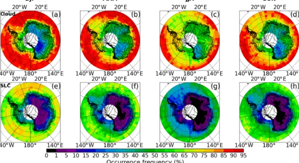
The geographical distributions of the total cloud and SLC fractions are shown as seasonal averages derived over 2007– 2010 in Fig. 5. They clearly show how the total SLC fraction distribution (Fig. 5e–h) differs from the total cloud fraction distribution (Fig. 5a–d). We first comment on the cloud frac-tion and then on the SLC fracfrac-tion.

Figure 5a–d show that the SO and the Antarctic seas have the largest cloud fractions as already demonstrated in pre-vious studies using other synergetic A-Train products (Ver-linden et al., 2011; Bromwich et al., 2012; Adhikari et al., 2012). There, the cloud fraction reaches values larger than 90 %. From summer to winter the cloud fraction decreases the most in the Weddell Sea and the Weddell Sea sector and in the Ross Sea (by an amplitude of ∼ 30 %). These are places where the sea ice formation extends the most equa-torward (Fig. 2k). Observing the highest continental cloud fractions over the WAIS is consistent with the presence of the ASL to the north of it, which brings moisture from lower latitudes to the slopes of WA coasts. There, the orography induces adiabatic cooling and cloud formation (e.g. Scott et al., 2017). The deepening of the ASL in winter (Fig. 2c) is associated with an increase in the cloud fraction over the WAIS (Fig. 5c), which is consistent with the intense mois-ture fluxes and higher cloudiness related to the sustained

cy-C. Listowski et al.: Antarctic clouds, supercooled liquid water and mixed phase 6779

Figure 5. Geographical distribution of the total cloud fraction (a–d) and the total SLC fraction (e–h) for each of the four seasons based on 2007–2010 averages.

clonic activity across the Amundsen and Ross seas (Nicolas and Bromwich, 2011), a process also observed along EA’s coasts (Dufour et al., 2019).

A salient feature is the minimum of the cloud fraction reached over the megadune region (75–82◦S, 110–150◦E) (e.g. Frezzotti, 2002), west of the Transantarctic Mountains. In fact, the minimum cloud fraction occurs around 140◦_E

longitude throughout the year. The largest value of this mini-mum occurs in winter (30 %–35 %). This region corresponds to the area with the largest subsidence of air on the plateau, as emphasised by Verlinden et al. (2011) (their Fig. 4). More generally, the lowest cloud fractions are found across the high-altitude terrain of the Antarctic Plateau, compared to the cloudier WAIS (by at least 20 % in absolute value). Outside of the megadune region, the cloud fraction in EA increases from 30 %–35 % in summer to 60 %–65 % in winter.

The SLC fraction geographical distribution (Fig. 5e–h) is in strong contrast to that of the cloud fraction, especially over the continent. In EA, the SLC fraction decreases sharply polewards and away from the coast in all seasons (Fig. 5e–h), following the increasing surface height. The SLC fraction is at most 10 % in summer over the plateau, decreasing to al-most 0 % during other seasons and especially in winter. WA shows, in comparison to EA, larger continental SLC tions in summer (30 %–40 % vs. 10 %–20 %). The SLC frac-tions are the largest over the ocean with an average value of ∼70 % (Fig. 5e). As for the cloud fraction, the strongest de-crease in offshore SLC fractions in winter occurs in regions where sea ice forms. In summer, the eastern Weddell Sea and the Weddell Sea sector have the largest SLC fractions (75 %– 80 %). The western Weddell Sea (60–40◦W) shows system-atically lower SLC fractions than the eastern Weddell Sea

(40–20◦W) and more particularly in summer, with a 12 % absolute difference in the SLC fraction (Fig. 5e).

To further emphasise the difference between cloud fraction distributions, we show the seasonal geographical distribution of the total all-ice, MPC and USLC fractions in Fig. 6. Re-call that all-ice, MPC and USLC fractions describe – when added up – the entire cloud fraction (Eq. 1). By consider-ing the all-ice fraction (Fig. 6a–d), we clearly highlight the enhancement of ice clouds over the WAIS from the summer season (20 %–25 %, Fig. 6a) to the winter season (∼ 65 %– 70 %, Fig. 6c). This feature is explicable by the deepening of the ASL (Fig. 2c) and the upper-level low-pressure sys-tem in the Ross Sea region (Fig. 2g). The increase in the all-ice fraction in winter on the WAIS and in EA close to Princess Elizabeth Land (Fig. 1) near the coasts at ∼ 90◦E is in agreement with the strengthening of the ASL and the other climatic low-pressure system located around 100◦E (Fig. 2c) and drives the increase in the cloud fraction (Fig. 5c).

The all-ice fraction distribution in winter (Fig. 6c) ranges between 45 % and 70 % across the whole continent, except west of the Transantarctic Mountains, where it is around 30 %. It is interesting to note that the cloud-depleted area observed in the cloud fraction over the megadune region is observed in the all-ice fraction throughout the year but not in the SLC fraction. This area is located downwind of the ASL (the upwind area being Marie Byrd Land, Fig. 4a) and of the upper-level low-pressure system of the RIS. The airstream of the ASL will meet with the Transantarctic Mountains and prevent moisture or cloudiness from progressing further.

West and east of the Amery Ice Shelf (AIS, Fig. 1), the all-ice fraction is larger than over it. At the same time the SLC fraction is actually larger over the AIS than in the

neighbour-ing areas of similar latitudes. This can be seen in all seasons. This is consistent with the presence of the depression in the land south of the AIS, where the absence of a sharp longitu-dinal gradient in the orography would allow (due to the lack of adiabatic cooling) for slower or delayed cooling and the liquid phase not to freeze.

The largest all-ice fractions each season happen to be where the orography is and southwards of places where the three climatic low-pressure systems are (see Sect. 2, and Fig. 2a–d). Hence, the all-ice fraction corresponds to oro-graphic clouds and fewer of those clouds occur over the large Weddell and Ross sea embayments (e.g. Fig. 5e). The Antarctic Peninsula (∼ 65◦W) also acts as a barrier to the dominant westerlies and triggers ice cloud formation through interaction between the airflow and the orography. The all-ice fraction is larger in that region than in areas over water nearby at similar latitudes. It can be already noticed that the spatial pattern of the sea ice fraction spatial distribution in winter is not similar to that of the all-ice cloud fraction dis-tribution, contrary to what is observed for the SLC fraction (for instance, compare the winter patterns of sea ice in Fig. 2o with the winter cloud and SLC distributions in Fig. 5c and g on one side and the winter all-ice distribution in Fig. 6c on the other side).

The MPC fraction (Fig. 6e–h) and the USLC fraction (Fig. 6i–l) are the largest in summer. There is an area of con-centrated higher USLC fraction in the eastern Weddell Sea in summer, which has no counterpart elsewhere in the Antarc-tic region (e.g. in the Ross Sea). Over the SO and the seas, the absolute difference between the average MPC fraction and USLC fraction is the largest in autumn (33 % vs. 20 %, Fig. 6f and j), while it is the smallest in spring (26 % vs. 23 %, Fig. 6h and l). This difference is 8 % in summer and 4 % in winter. As for the SLC fraction, the MPC and USLC fractions are lower on the continent and particularly in EA, where they decrease polewards. Interestingly, these fractions show no significant differences between each other on the continent, in contrast to what is observed over seas. This will be investigated and discussed further below.

4.2 Vertical distribution of clouds and supercooled liquid water

As a complement to the geographical distribution of clouds, we now investigate their vertical distribution with a focus on the SLW. We show the 4-year average transects (at the 60 m vertical resolution) in the three latitudinal bands de-fined in Fig. 4d, aimed at roughly describing the SO (60– 65◦S), the coastal areas (65–75◦S) and the interior of the continent (75–82◦S). Transects were built for the cloud frac-tion (Fig. 7a), the SLC fracfrac-tion (Fig. 7b), the MPC fracfrac-tion (Fig. 8a) and the USLC fraction (Fig. 8b). In Fig. 8, isotherms built using the ECMWF temperatures stored in the DARDAR product indicate the average temperature at which MPCs and USLCs form. Similar transects of the cloud fraction as the

ones shown in Fig. 7 are discussed in Adhikari et al. (2012) for 2007–2010 and in Verlinden et al. (2011) for 2007–2009. However, we show the 4-year average for the cloud fraction to put the other transects into context. We limit ourselves to the low and middle altitudes as this is where all SLC form. The average topography in each transect is indicated by the solid white line. Since the topography is not homogeneous along any given meridian within each latitudinal band, the number of effective footprints per altitude level will change along any meridian in the coastal and the interior transects. In order to show a smooth pattern of cloud vertical distribu-tion we divide the number of occurrences of any cloud type in any three-dimensional grid box by the effective number of footprints in it (this number equals the number of overpasses above that grid box if the grid box is above the surface, and zero, if it is below the surface). In doing so, when averag-ing to build the transect, we account for the actual reduction in footprints along each meridian at altitude levels that are partly above and partly below the surface. Note that, since the fractions are derived in each of the 60 m vertical bins, they are lower than the ones derived for the geographical dis-tributions, for which the occurrences of clouds were derived over the tropospheric column whatever their altitude.

The reduced statistics due to the radar blind zone and the lidar signal extinction across the Antarctic clearly appears in the resulting transects for the cloud fraction at ∼ 500 m a.s.l. (e.g. Fig. 7Aa). This is illustrated and discussed in Ap-pendix A with Fig. A1. There is a sharp reduction in the low-level cloud fraction below ∼ 500 m a.s.l., which corre-sponds to the lesser ability to detect clouds because of the radar blind zone. Satisfyingly, despite a reduction by up to 40 % of the number of valid radar observations from 1 km to 500 m a.s.l. (Fig. A1a), no discontinuity appears in the verti-cal transects above 500 m a.s.l. (Fig. 7Aa). This suggests that the vertical distribution of cloud fraction is well reproduced above this altitude and that it is legitimate to use 500 m as a lower-altitude cut-off for the geographical distributions in-troduced in the previous section.

4.2.1 Cloud vertical distribution

The highest vertical cloud fractions (70 %) occur at low alti-tudes in the SO transects (Fig. 7Aa, d, g and j). The maximum of the summer cloud fraction occurs across the boundary be-tween the Weddell Sea sector and the Indian sector (20◦E) and in autumn in the Indian sector and the Amundsen–Ross sector (Fig. 7Aa and d). In spring, the latter has the highest occurrences of low-level clouds. To the east of the Antarc-tic Peninsula (∼ 65◦W, hereafter called the peninsula), north of and in the Weddell Sea (60–25◦W), the cloud fraction is halved at each altitude level between 0.5 and 2 km a.s.l. in winter (20 %–30 % Fig. 7Ag and h) compared to sum-mer (40 %–60 % Fig. 7Aa and b). This reduction is less pro-nounced above 2 km a.s.l. To the west of the peninsula, the cloud fraction is hardly changed at similar altitudes. Hence,

C. Listowski et al.: Antarctic clouds, supercooled liquid water and mixed phase 6781

Figure 6. Geographical distribution of the total all-ice cloud fraction (a–d), MPC fraction (e–h) and USLC fraction (i–l) for each of the four seasons based on 2007–2010 averages.

this drop in the cloud fraction induces a dramatic difference in the winter and spring longitudinal distributions of low-level clouds across the peninsula, between the west (45 %– 55 %) and the east (20 %–30 %) of the mountain chain. Ad-ditionally, and whatever the season (Fig. 7b, e, h and k), there is a ∼ 20 % absolute difference in the mid-level cloud frac-tions between both sides of the peninsula, i.e. well above the highest peak of the peninsula (∼ 2.5 km). East of the penin-sula, the lowest low-level cloud fractions in winter and spring coincide with the largest sea ice fractions (Fig. 4k and l).

In EA, east of the AIS (around 90–100◦E, Fig. 7Ah) a local increase in the vertical extension of coastal cloud frac-tion occurs in winter, at altitudes up to 6 km a.s.l. This fea-ture in the vertical distribution of clouds occurs while the cli-matic low-pressure system located off the coast is strength-ened (Fig. 4c). This low-pressure system is the weakest in summer (Fig. 4a), and the cloud fraction is also at its lowest (∼ 25 %) (Fig. 7Ab). This seasonal variation is seen during each year taken separately. South of the AIS (∼ 70◦E), the cloud fraction is lower than immediately to the east and to the west of the AIS (Fig. 7Ae, h and k). This is the effect of the land depression there, preventing the orographically induced cloud formation from occurring.

Generally, the cloud vertical extension follows the air mass interactions with the coastal topography. This is also clearly visible in the interior transects (Fig. 7Ac, f, i and l) around 100◦W, on the WAIS. There, the ASL brings moisture from lower latitudes, triggering cloud formation through adiabatic cooling on the steep coasts. In winter the vertical extension of clouds lead to values of 45 % and 30 % at 2 km and 6 km a.s.l. against 40 % and 10 % in summer. Hence, higher clouds oc-cur at higher altitudes in winter and this is consistent with the deeper ASL and the contraction of the westerly circu-lation towards the coast (Fig. 4c). In EA, the area of lowest cloud fraction (∼ 5 %–10 %) is visible around 140◦E consis-tently with observations made by Verlinden et al. (2011) over 2007–2009. It is the area of largest subsidence and also im-mediately west of the Transantarctic Mountains, which pre-vents moisture or cloudiness from WA entering EA. The land depression extending poleward from the AIS is the area of maximum cloud fraction in the interior in winter (∼ 70◦E, Fig. 7Ac, f, i).

4.2.2 Supercooled liquid-water vertical distribution The largest SLC fractions are consistently found in the low-est (warmlow-est) atmospheric layers, below 2 km altitude in the Southern Ocean transect (Fig. 7Ba, d, g, and j) and the coastal

Figure 7. (A) Four-year (2007–2010) average seasonal vertical transects of the cloud fraction, spatially averaged over three latitudinal bands defined in Fig. 4d (SO stands for Southern Ocean). One column corresponds to one latitudinal band, showing the four seasons. Each line corresponds to one season. (B) Same as (A) for the SLC fraction. The white line is the average surface elevation in the latitudinal band.

C. Listowski et al.: Antarctic clouds, supercooled liquid water and mixed phase 6783

Figure 8. (A) Same as Fig. 7A but for the MPC fraction. (B) Same as (A) but for the USLC fraction. Additionally, isotherms are shown every 5◦C (dotted white lines) and they are labelled but ignore the minus sign in the temperature value. The warmest temperature shown in all panels is −5◦C. In plots (Aa) to (Ak) and (Ba) to (Bk) (SO and coastal transects) isotherms are shown down to −25◦C only, while for the interior transects they are shown down to −35◦C.

regions (Fig. 7Bb, e, h, and k). The largest SLC fractions over the largest oceanic area are found in autumn across the Weddell Sea sector and the Indian sector (0–70◦_{E) at}

1–1.5 km altitude (Fig. 7Bd). This corresponds to an area of preferred MPC formation compared to USLCs (compare transects Fig. 8Ad and Bd). In the coastal transect the Wed-dell Sea is an area of enhanced SLC formation (60–25◦W, Fig. 7Bb). This maximum is principally due to the increase in the USLC fraction there (Fig. 8Bb) rather than to the MPC fraction (Fig. 8Ab). This already appeared in the USLC frac-tion geographical distribufrac-tion (Fig. 6i). This suggests that the Weddell Sea is an area more prone to maintain layers of su-percooled liquid with no significant glaciation process. There is a clear cut in the SO zonal distribution of the SLC frac-tions at the northern tip of the peninsula (∼ 60◦W), causing an asymmetry in this distribution. Lower altitudes (a.s.l.) are reached by SLCs to the east of the peninsula compared to the west. This is particularly visible outside summer months (Fig. 7Bd, g, and j) and can be explained by the lower surface temperatures on the eastern side of the peninsula, which is well documented in the literature (e.g. Morris and Vaughan, 2003). Also note the changes in the isotherms, which have lower altitudes to the east of the peninsula (Fig. 8Aa, d, g and j).

Over water, the largest USLC fractions generally occur between 0.5 km and 1 km a.s.l., and the largest vertical ex-tent of the largest USLC fractions occurs in the Weddell Sea (Fig. 8Bb). The maximum MPC fractions are located between 1 km and 1.5 km a.s.l. with no MPCs detected be-low 500 m a.s.l. The isotherms indicate the average tempera-tures at which MPCs and USLCs form. In the SO transect and in the coastal transect, the largest MPC fractions oc-cur between −15 and −5◦_{C and more particularly between}

−15 and −10◦C. In the SO transect, USLCs occur at tem-peratures above −5◦C in summer (Fig. 8Ba) and between −10 and −5◦C in other seasons (Fig. 8Bd, g and j). The high USLC fractions in the Weddell Sea in summer between 0.5 km and 1 km a.s.l. occur at temperatures between −10 and −5◦C (Fig. 8Bb).

In the interior transects, the SLC fraction is the largest above the WAIS (∼ 100◦W) and the RIS (170◦E–150◦W) throughout the year (Fig. 7Bc, f, i, and l). In EA, on the plateau, SLCs occur almost exclusively in summer at tem-peratures down to −35◦C. The SLC fraction maximises in summer at 3 km a.s.l. over the WAIS and below 500 m a.s.l. above the RIS (Fig. 7Bc), mainly in the form of USLCs (compare Fig. 8Bc and Ac). Over the WAIS, this maximum occurs at average temperatures between −23◦_{C and −20}◦_C

(Fig. 8Bc) and around −25◦C in other seasons. It is reminis-cent of quasi-steady-state mountain-wave orographic clouds displaying supercooled droplets down to −33◦C with no ice (Heymsfield and Miloshevich, 1993). However, satellite ob-servations do not allow a statement to be made on the life-time of such a feature. Note that low-level SLCs that are cat-egorised as USLCs in the radar blind zone above the RIS

(be-low 500 m a.s.l.) could actually be MPCs. Silber et al. (2018), who investigated liquid-bearing clouds with ground-based measurements at McMurdo Station (167◦_{E) at the edge of}

the RIS throughout the year 2016 did not differentiate be-tween pure and mixed SLC layers. Thus, we cannot deter-mine the preferred formation of USLCs or MPCs at very low altitudes there. In EA, the presence of SLCs is evidenced in summer (Fig. 7Bc), while no SLCs are detected over the plateau in winter, except where the depression of the land south of the AIS is (Fig. 7Bi). There, poleward intrusion of moisture and cloudiness from the coastal areas would cause enhanced SLC fractions (Fig. 7Ai).

Unlike for the cloud fraction, no discontinuity occurs in the SLC fraction vertical distribution close to the surface, es-pecially over seas (Fig. 7B). This suggests that the statistics of the SLC fraction vertical distribution close to the surface is not much affected by the reduced statistics due to the li-dar extinctions (∼ 80 % near the surface, Fig. A1d). Above land, some spurious SLC fraction enhancements appear at the surface on very rare occasions, though (e.g. Fig. 7Bc, at ∼50◦E). It is also interesting to note that the maximum in the vertical MPC fraction occurs above 1 km height above ground level in the transects (Fig. 8A), suggesting that the decrease in MPC occurrences below 1 km is rather real and not an artefact of the 40 % reduced statistics (at 500 m a.s.l.) caused by the radar blind zone. The consequence of this is that the picture given by the DARDAR-MASK products of the MPC fraction and the USLC fraction is representative of their actual averaged distribution down to 500 m a.s.l. and possibly down to the surface for the SLC fraction at least (which does not rely on the radar signal). Hence, using a 500 m lower altitude cut-off for deriving the distributions of MPC and USLC fractions seems legitimate despite the re-duced statistics.

4.3 Monthly time series over specific Antarctic regions 4.3.1 Total cloud and phase fractions

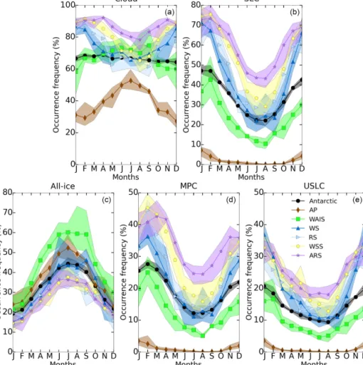
We now spatially average the geographical distribution of the total cloud fractions presented in Sect. 4.1 over distinct areas defined in Fig. 4c. In doing so, we increase the statistics com-pared to a single grid box, while we pin down the monthly evolution in these regions. The geographical areas investi-gated are called WSS (in the Weddell Sea sector), ARS (in the Amundsen–Ross sector), WS (in the Weddell Sea), RS (in the Ross Sea), AP (the Antarctic Plateau) and the WAIS (Fig. 4c and Table 1). We also show the monthly time series for the whole Antarctic region (60–82◦S). Note that ARS and WSS are of similar sizes, as WS and RS. Figure 9 shows the monthly evolution of several total fractions: cloud (a), SLC (b), all-ice (c), MPC (d) and USLC (e). The shaded ar-eas indicate the 4-year maximum and minimum monthly av-erage values as an indication of the amplitude of interannual variability.

C. Listowski et al.: Antarctic clouds, supercooled liquid water and mixed phase 6785

Figure 9. Four-year (2007–2010) average monthly time series of the total cloud fraction (a), SLC fraction (b), all-ice fraction (c), MPC fraction (d), and USLC fraction (e). See Sect. 3.2 for the definition of the cloud categories. The different colours correspond to the different investigated regions (see map in Fig. 4c): WSS (in the Weddell Sea sector), ARS (for the Amundsen–Ross sector), WS (in the Weddell Sea), RS (in the Ross Sea), the WAIS (on the West Antarctic Ice Sheet) and AP (Antarctic Plateau). The shaded areas indicate the amplitude between the monthly minimum and maximum encountered over the years from 2007 to 2010.

A striking feature is the constant average cloud fraction throughout the year for the whole Antarctic region, around 68 % (black lines in Fig. 9) (Fig. 9a). When considering spe-cific regions, different patterns appear. Generally, the maxi-mum cloud fraction over continental regions occurs in winter and the minimum in summer, while the opposite occurs over oceanic regions. The cloud fraction derived for ARS shows the lowest amplitude of variation. It decreases from 90 % to 92 % in mid-autumn and throughout the winter and reaches a minimum of 78 % by the end of it. It increases again, reach-ing a second maximum around 90 % in late sprreach-ing. A similar pattern appears for WSS, with a stronger decrease throughout winter, down to 65 %. This is consistent with the larger sea ice fractions observed in that area in JJA (Fig. 2o) and SON (Fig. 2p) and can be related to the likely reduced moisture flux into the atmosphere. WS and RS show the same pattern of a decreasing cloud fraction, starting from a maximum in summer. However, the cloud fractions are on average lower in winter over RS (∼ 60 %) than over WS (∼ 70 %). On the

continent, the WAIS shows a slight increase in cloud frac-tion from summer (60 %) to winter (75 %) before decreasing abruptly from September to October. A much clearer trend emerges over the AP with a steady increase in cloud fraction from summer to winter and a maximum in July. It is the area where the seasonal cycle has the largest amplitude of varia-tion (as already noted by Verlinden et al., 2011, using vertical transects). The same abrupt decrease in the cloud fraction as over the WAIS is noticeable between September and Octo-ber.

The monthly evolution of the SLC fraction (Fig. 9b) is a general decrease from summer to winter with a minimum reached in August, before increasing again. This seasonal cycle is not biased by one of the lidar signal extinctions, which has occurrences that are equal to or lower than the SLC occurrences and follow the same pattern (Appendix A, Fig. A2). As a lidar signal extinction will happen below a SLC detection, this is expected. Some of the SLCs may be detected just above the 500 m lower altitude cut-off, so that

the SLC occurrence is then counted, but the extinguished area below is missed in the statistics. Extinction or attenu-ation of the lidar signal can also happen because of optically thick ice clouds, and this is why the occurrences of extinc-tions and attenuaextinc-tions are almost as important in the winter as they are in the summer over the WAIS (Fig. A2). Overall, the seasonal cycle of the SLC fraction above 500 m above the surface is not biased by the lidar extinctions. The largest SLC fractions occur in ARS and WSS (both 75 %) in sum-mer against 40 % and 30 % in winter. The lowest values of the SLC fraction are observed above the continental areas. The SLC fraction in the WAIS is 40 % in summer and 10 % in winter. The plateau has few but non-negligible SLC oc-currences, with ∼ 10 % in January, and none by the end of winter and early spring. The relatively simple SLC fraction seasonal cycle points to the temperature seasonality as being one of the main drivers everywhere in the Antarctic (colder temperatures favour more glaciation in clouds).

Contrary to the cloud fraction evolution, the all-ice cloud fraction shows the same evolution over each area, increasing from the end of the summer to the winter (Fig. 9c). ARS and WSS show similar values ranging from 15 % to 35 %, while the WAIS reaches the largest 4-year average of 60 %. The AP has the second largest values of all-ice fractions in win-ter (50 %). This fraction is lower than in the WAIS and can be explained by the ASL located off the WAIS coast, con-tributing to a direct inflow of moisture (and cloudiness). Note the almost identical evolution for the cloud and all-ice frac-tions over the AP, showing the almost exclusive presence of ice clouds there. These fractions only differ during the sum-mer months, when SLC fractions are not negligible (∼ 10 %, Fig. 9b).

A striking difference appears between the MPC and the USLC fractions (Fig. 9d and e) when considering the tran-sition from beginning of summer to autumn. All regions – with the exception of the AP – show a local maximum of the MPC fraction in late summer or early autumn before a decrease in the following months, with a minimum reached around August. Conversely, the USLC fraction shows a steep decrease over the same period, which starts in January. This difference suggests that the glaciation process converting the supercooled liquid to a mixed phase follows a distinctly dif-ferent cycle from the one describing the mere occurrence of supercooled liquid (although the former is obviously related to the latter). These differing behaviours are readily observed by comparing the Antarctic averages (solid black lines) in Fig. 9d and e. The differences in MPC fractions between ma-rine areas (ARS, WSS, WS and RS) are larger than the dif-ferences in the USLC fraction between the same areas. For instance the USLC fractions are within a 5 % range of val-ues except during winter (8 %), while the MPC fractions can differ by more than 15 %. This points to larger regional dif-ferences in the glaciation process (and occurrences of MPC) than in the mere occurrences of USLCs.

4.3.2 Cloud and phase fractions at low, middle and high levels

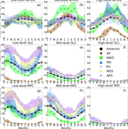
To look further into the details of the monthly evolution of the different cloud fractions, we divide them into low-level, mid-level and high-level fractions, as defined in Sect. 3.2. Figure 10 shows the all-ice fractions (a–c), the SLC fractions (d–f) and the MPC fraction (g–i). Since the addition of the all-ice and the SLC fractions gives the cloud fraction, it is easy to infer what the dominant component of the cloud frac-tion is and we do not show the cloud fracfrac-tion here, although we still refer to it.

Over the continent, the monthly variability of the cloud fraction is primarily driven by the mid-level and high-level all-ice clouds (Fig. 10b and c). The monthly variability is within a 30 % range and 35 % range for mid- and high-level all-ice fractions on the WAIS, and 30 % and 15 % over the AP. Regarding the AP, the mid-level clouds can virtually be considered high clouds (in comparison to the oceanic re-gions) since the average altitude of the plateau is 3 km a.s.l. The evolution of the continental mid-level and high-level all-ice cloud fractions appears to be the same in both WAIS and AP, changing from a minimum in summer to a maximum in winter. This is consistent with the increases in cyclogen-esis and depressions offshore in that season (e.g. King and Turner, 1997), leading to more intrusions of weather sys-tems over the continent. The monthly evolution of continen-tal clouds is essentially driven by the all-ice clouds. The mid-and high-level clouds detected over the WAIS mid-and the AP are almost exclusively of the all-ice type given the much smaller mid-level SLC fractions (0 % and ≤ 10 % for AP and WAIS) compared to the mid-level all-ice fractions (20 %–50 % and 10 %–40 % for AP and WAIS) on one side and the almost null high-level SLC fraction (except over ARS) compared to the all-ice fractions on the other side.

Interestingly, over water (WS, RS, WSS and ARS regions) the mid-level cloud fraction shows almost no monthly vari-ability compared to the low-level cloud fraction and the high-level cloud fraction (not shown). Mid-high-level cloud fractions are always within a 10 % range of values in ARS, WSS, RS and WS. We can understand the absence of monthly varia-tion for mid-level cloud fracvaria-tions over marine areas, since the ∼ 13 % increase in mid-level all-ice fraction (Fig. 10b) is almost compensated by a similar decrease in the SLC frac-tion (∼ 10 % decrease, Fig. 10e). This may be explained by the mid-level liquid phase being more often converted or re-placed by ice in the winter season. Over water, the low-level cloud fractions are within a ∼ 40 % range of values in WS, ∼30 % in RS, ∼ 35 % in WSS and ∼ 20 % in ARS and this variability is caused by the SLC fraction (Fig. 10d). High-level cloud fractions are driven by the all-ice fraction and are within a ∼ 25 % range of values in WS, ∼ 15 % in ARS and WSS, and ∼ 10 % in RS. This demonstrates that the vari-ability of the cloud fractions over water is firstly due to the low-level liquid-bearing clouds, which dominate the cloud

C. Listowski et al.: Antarctic clouds, supercooled liquid water and mixed phase 6787

fraction, and secondly to the high-level all-ice clouds, while mid-level clouds have little influence. Over marine regions (WS, RS, WSS, ARS), the monthly variability of the all-ice fraction (Fig. 10a–c) is largely driven by the mid- and high-level all-ice clouds (Fig. 9b and c), pointing to the increased cyclonic activity and number of frontal systems in winter (as for the general cloud fraction).

The monthly evolution of the low-level MPC fraction clearly differs from the low-level all-ice fraction, but also from the low-level SLC fraction. Over marine areas, little monthly variation in the low-level all-ice fraction occurs throughout the year in comparison to the low-level MPC fraction, suggesting that different factors affect their respec-tive formation and evolution. More particularly, the monthly variation observed for the low-level all-ice fraction in WS, WSS and ARS is in a range of values of 5 % (10 % for RS), while the monthly variations in low-level MPC frac-tions are within a larger range of values, i.e. 20 % for WSS, 15 % for WS and RS, and 10 % for ARS. The largest part of the total USLC fraction is driven by the low-level USLCs (not shown), which does not show a local maximum at the end of summer or beginning of autumn, explaining the dif-ferent patterns between the low-level SLC (Fig. 10d) and MPC (Fig. 10g) seasonal cycles. Finally, Fig. 10g demon-strates that the singular evolution of the MPC fraction from summer to autumn (Fig. 9d) is due to the low-level MPC. The mid-level MPC fraction does not display any similar lo-cal maximum in autumn. The particular monthly variation in the low-level MPC fractions points to a seasonal cycle of the glaciation process, involving interactions with the surface and/or the lowest layers of the troposphere. Note that, given the absence of seasonality in the radar clutter occurrences (Fig. A2), identifying ice in SLCs to assess the existence of a mixed-phase cloud seasonality is not biased.

Figure 11 shows the monthly time series of the in-cloud temperature and water vapour mass mixing ratio at the top (Ttop and Qtop) of the low-level MPCs and USLCs, as well as the ones at the surface (T2m and Q2m) below where these clouds occur. The seasonal cycles of Ttop and T2m show a similar pattern to that of the SLC fraction suggesting the temperature as being the main driver of the SLC fraction evolution. The decrease in Qtop and Q2m is a direct con-sequence of the formation of sea ice and the reduction in moisture coming from the sea surface. Ttop of USLCs are larger than those of the MPC layers as the latter form at higher altitudes on average and have some active glaciation process suggestive of these lower temperatures. Note that, in the DARDAR-MASK, the two criteria using temperature in the identification of supercooled liquid is −40◦C, taken as the homogeneous nucleation temperature, below which the lidar backscatter will be considered to come from highly con-centrated small ice crystals, and 0◦C, above which the liquid layer will be considered warm liquid (Ceccaldi et al., 2013). Apart from that it is the combination of lidar and radar ob-servations that determines whether or not liquid and ice are

simultaneously present. Hence, our observations of system-atic higher average temperatures (and lower altitude – from Sect. 4.2) of the USLC are, while being independent, in line with the identification of these layers. Marine SLC top tem-peratures range between −22 and −10◦C. Continental SLC top temperatures range between −38 and −22◦C. The aver-age lowest SLC top temperature occurs on the plateau (−35 in summer and −38◦in winter). The statistics based on the highest number of samples, i.e. those for the whole Antarc-tic region (black lines in Fig. 11a), give a 1.5–2◦C warmer Ttop for USLCs than for MPCs. This temperature difference is significant at the 99.9 % level (using a t test), while the differences between Qtop for MPCs and USLCs is signif-icant at the 90 % level only. There are no statistically sig-nificant Antarctic-wide differences in the near-surface tem-perature and water vapour mixing ratio between the MPCs and USLCs (Fig. 11c and d). This shows that the average near-surface conditions are the same for both types of SLC and more particularly over water. The only exception is the winter near-surface temperature on the plateau, which corre-sponds to extremely low and almost null SLC occurrences (Fig. 10g and j).

4.4 Comparison with ground-based measurements from the coast to the interior

The DARDAR products were validated in the Arctic by Mioche et al. (2015) using comparisons with a ground-based micropulse lidar. In this section we use the geo-graphical cloud fraction distributions derived above to make comparisons with ground-based measurements of different sorts (cloud fraction, precipitation, SLC fraction) taken over 2007–2010 in Antarctica.

4.4.1 Ceilometer cloud base observations at Rothera and Halley between 2007 and 2010

In order to get a better perspective of the monthly evolution of cloud fraction illustrated by Fig. 9a, we performed qualita-tive comparisons with ceilometer data collected at the British Antarctic Survey’s stations Rothera and Halley (Fig. 1) for the period 2007–2010. These were introduced in Sect. 3.3. We compare these with our low-level cloud fraction as the average height of cloud bases detected by the ceilometers is ∼ 1600 m at Rothera and ∼ 1000 m at Halley. When us-ing the data from the ceilometers, we plot cloud base occur-rences as measured starting from above the surface (> 0 m) and from above 500 m above the surface (> 500 m). In or-der to have enough monthly statistics from the satellite over-passes we extend the analyses to larger regions than the grid box containing the respective station (see Fig. 4a). Hence, in addition to the stations’ grid boxes we derive the low-level cloud fraction using – for Rothera Station – the Belling-shausen sea (i.e. upwind of the station) and – for Halley – the Weddell Sea (off the Brunt Ice Shelf where Halley sits).