The effect of a plasma sheath on hypersonic flight communications

The Effect of a Plasma Sheath

on Hypersonic Flight

Communications

by

Hiroshi Taneda

S.B. Aeronautics, Tokyo University, 1981 S.M. Aeronautics, Tokyo University, 1983 SUBMITTED IN PARTIAL FULFILLMENT OF THE

REQUIREMENTS FOR THE DEGREE OF

Master of Science in

Aeronautics and Astronautics

at the

Massachusetts Institute of Technology

May 1990

@1990, Hiroshi Taneda, All Rights Reserved

The author hereby grants to MIT permission to reproduce and distribute copies of this thesis document in whole or in part.

Signature of Author

Department of Aeronautics and Astronautics May 1990

Certified by

topfessor Daniel E. Hastings, Thesis Supervisor ,

*Departipent of AerpnaItics and Astronautics

Accepted by

' _{.. Proer Harold Y. Wachman, Chairman} Department Graduate Committee

INST.

JUN 1

9 199

The Effect of a Plasma Sheath

on Hypersonic Flight

Communications

by

Hiroshi Taneda

Submitted to the Department of Aeronautics and Astronautics

in partial fulfillment of the requirements for the degree of

Master of Science in Aeronautics and Astronautics

The attenuation of electromagnetic waves propagating through a plasma sheath sur-rounding a sigle-stage-to-orbit vehicle with a scramjet was estimated. The forebody of the vehicle is simulated by a two dimensional wedge and the chemical composition and the effective dielectric coefficient in the high temperature air associated with the shock and the boundary layer over the wedge are calculated. The flow anal-ysis includes the finite rate chemistry in the inviscid region and assumes chemical equilibrium in the boundary layer.

Three different typical trajectories are selected and the effects of velocity, wedge angle, and wall temperature on the attenuation are studied. The results show that the attenuation becomes significant above Mach 16 for radio frequencies below X band. The critical radio frequency decreases with increasing altitude. The increase in wedge angle above 10" increases the attenuation drastically while the effect of wall temperature is relatively small for the temperature range between 1000 K and 2000 K.

Thesis Supervisor: Professor Daniel E. Hastings Associate Professor of Aeronautics and Astronautics

Acknowledgements

I wish to express my thanks to my thesis supervisor Prof. Daniel E. Hastings for his guidance and numerous helpful suggestions. His strong support based on profound physical insights and enthusiasm about the topic will always be remembered and appreciated. I also would like to thank Prof. Martinez-Sanchez, who has provided much of the approach of this thesis and valuable suggestions. It has been my great pleasure to work with outstanding fellow students. I wish to express my special thanks to Rodger Biasca, who has provided helpful suggestions on the computation of high temperature air chemistry. I am also grateful to all of my officemates and coworkers for having provided valuable supports and wonderful company.

Contents

3.1 Inviscid Chemically Nonequilibrium Flows 3.1.1 Governing Equations ...

3.1.2 Finite Rate Chemistry ... 3.2 Boundary Layer ... 3.2.1 Self-similar Solutions . . . . 3.2.2 Numerical Procedures . . . . 4 The 4.1 4.2

Propagation of Electromagnetic Waves in Non-uniform, Isotropic Plasma . . . . Attenuation ... Plasmas 5 Numerical Results 5.1 Flow Results ... 5.1.1 Inviscid Region... 5.1.2 Boundary Layer ...

5.2 Attenuation of Electromagnetic Waves . . . . .

10 10 13 27 27 29 |

. . . .

...

...

...

. . . .

. . . .

6 Conclusions 60

A Reaction Model of High Temperature Air 65

B Calculation of Equilibrium Composition 68

C Effective Collision Frequency 70

List of Figures

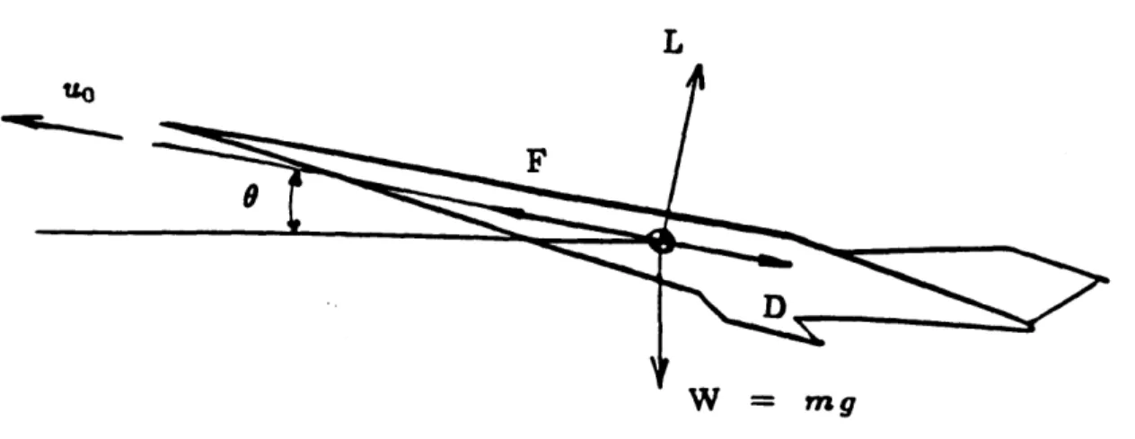
2.1 Force Diagram for Hypersonic Vehicle . ... . ... 11

2.2 Typical Trajectories and Constant Dynamic Pressure ... 14

3.1 _{Schematic of the flow over a wedge ... ... 26}

3.2 _{Schematic of nonequilibrium shock over a wedge . ... 26}

3.3 _{Simplified flow model over a wedge ... 26}

4.1 _{Schematic of Electromagnetic Wave Propagation over a Wedge . . . . 30}

5.1 _{Nonequilibrium species distributions behind a shock at V=3.0 Km/s . 34} 5.2 Nonequilibrium species distributions behind a shock at V=4.0 Km/s . 34 5.3 _{Nonequilibrium species distributions behind a shock at V=5.0 Km/s . 35} 5.4 _{Nonequilibrium species distributions behind a shock at V=6.5 Km/s . 35} 5.5 _{Nonequilibrium species distributions behind a shock at V=7.5 Km/s . 36} 5.6 _{Effect of trajectory on nonequilibrium species distributions behind a} shock at V=6.5 Km/s ... ... 37

5.7 _{Effect of wedge angle on nonequilibrium species distributions behind} a shock at V=6.5 Km/s ... . . ... 38

5.8 _{Velocity and temperature profiles in a boundary layer at V=3.0 Km/s 40} 5.9 _{Species concentrations in a boundary layer at V=3.0 Km/s ... 40}

5.10 Velocity and temperature profiles in a boundary layer at V=4.0 Km/s 41 5.11 Species concentrations in a boundary layer at V=4.0 Km/s ... 41

5.12 Velocity and temperature profiles in a boundary layer at V=5.0 Km/s 42 5.13 Species concentrations in a boundary layer at V=5.0 Km/s ... 42

5.14 Velocity and temperature profiles in a boundary layer at V=6.5 Km/s 43

5.15 Species concentrations in a boundary layer at V=6.5 Km/s ... 43

5.16 Velocity and temperature profiles in a boundary layer at V=7.5 Km/s 44 5.17 Species concentrations in a boundary layer at V=7.5 Km/s ... 44

5.18 Effect of trajectory on Velocity and temperature profiles in a boundary

layer at V=6.5 Km/s ... ... 46

5.19 Effect of trajectory on concentrations in a boundary layer at V=6.5

K m /s _{. . . ... . . . . 47}

5.20 Effect of wedge angle on Velocity and temperature profiles in a

bound-ary layer at V=6.5 Km/s ... 48

5.21 Effect of wedge angle on concentrations in a boundary layer at V=6.5

K m /s _{. . . .. . .. 49}

5.22 Effect of wall temperature on Velocity and temperature profiles in a

boundary layer at V=6.5 Km/s ... 50

5.23 Effect of wall temperature on concentrations in a boundary layer at

V=6.5 Km/s ... _{... 51}

5.24 Effect of trajectory on the attenuation of electromagnetic waves . . . . 55 5.25 Effect of wedge angle on the attenuation of electromagnetic waves . . 56

5.26 Effect of wall temperature on the attenuation of electromagnetic waves 57 5.27 Effect of trajectory on the attenuation of electromagnetic waves at 1

GHz ... . . ... . _{... . 58}

5.28 Effect of wedge angle on the attenuation of electromagnetic waves at 1 G H z . . . .... . . . . ... . . . .. 58 5.29 Effect of wall temperature on the attenuation of electromagnetic waves

List of Tables

5.1 Calculation parameters ... ... 33

A.1 Reaction model of Dunn and Kang . ... ... 66 D.1 Polynomial coefficients for thermodynamic data in equilibrium . . . . 74

Chapter 1

Introduction

Inspired by the National Aero-Space Program, which started in 1985 in the United States, research on hypersonic flight has been actively pursued in various nations.

This hypersonic research has been aimed mainly at the development of a reusable

hypersonic vehicle with a supersonic combustion ramjet or SCRAMJET.

One of the most challenging concepts of this type of vehicle is the Single Stage

To Orbit vehicle or SSTO vehicle which would take off horizontally and fly up to orbital speeds in the atmosphere. A transatmospheric air-breathing vehicle, which

needs to provide sufficient air for the engine opperation, must be accelerated at relatively lower altitudes compared with the conventional rocket boosters. On the

other hand, in order to avoid excessive dynamic pressure and aerodynamic heating

for the structures and materials, higher altitudes are desirable.

Because of these constraints, the trajectory of the SSTO vehicle will be

con-strained into a very narrow region. An important question which should be taken into account for the trajectory is the interference between the electromagnetic waves used for communication and the plasma sheath around the vehicle.

A vehicle flying in the atmosphere at high velocities becomes surrounded by re-gions of ionized gas that affect the propagation of electromagnetic waves to and from the vehicle. The kinetic energy in a hypersonic free stream is converted to the internal energy of the gas across the strong bow shock wave, creating very high temperatures in the shock layer near the nose. If the temperature is high enough,

ionization is present and a large number of free electrons are produced throughout the shock layer.

Downstream of the nose region, a boundary layer grows along the surface of the vehicle. Since the Mach number at the outer edge of the boundary layer is still high, the intense frictional dissipation within the hypersonic boundary layer creates high temperatures and causes chemical reactions.

The ions and electrons produced in the high temperature air around the vehicle create a plasma sheath, which interacts with electrcmagnetic waves propagating to and from the vehicle. If the attenuation of the electromagnetic waves due to the plasma sheath is excessively high, then a communication blackout occurs.

The problem of communications blackout and the flow analysis related to this problem were extensively studied in the 1950s and 1960s mainly for reentry vehicles such as the Apollo[1,2,3]. Since a reentry vehicle usually has a blunt body, these stud-ies mainly focused on the analysis of the inviscid ionized gas over a blunt nose. The

SSTO vehicle, however, will have a slender body and the effect of a boundary layer

is expected to be much more important. The trajectory at relatively low altitudes is also a clear difference from other reentry vehicles.

In order to evaluate the interference between the electromagnetic waves and the plasma sheath, it is necessary to estimate the flow properties around the vehicle. The accurate estimation of the flow around the actual configuration requires computa-tions which solve the full 3-D Navier Stokes equacomputa-tions including a chemical model. However, these computations, which need an extremely large computation time even with the most advanced computers, are not adequate for the parametric study in the wide range of the flight conditions while the vehicle configuration is not well deter-mined yet. Therefore this thesis only considers very simple configurations and focuses on the general effects of the altitude, velocity, shock angle and wall temperature.

Since the major chemical reactions are caused by the strong shock wave which is generated by the forebody, this thesis only considers the flow regions around the forebody. Although no specific configuration is determined yet, the typical concepts of the SSTO vehicle have a slender forebody with a small bluntness at the nose. In

this thesis, two-dimensional wedges with a relatively small vertex angle are examined as the forebody geometry. Actual vehicles,however, have always some finite bluntness at the nose and a large number of electrons may be produced at the stagnation region. Since this effect of stagnation region is not taken into account in the wedge model, the flow analysis is only valid at the location which is sufficiently downstream from the nose. By ignoring the finite bluntness, the flow model may underestimate the electron density near the nose.

The goals of this thesis is to estimate the degree of attenuation of electromag-netic waves propagating to and from the SSTO vehicle and to evaluate the effects of trajectory, velocity, wedge angle, and wall temperature. In chapter 2, the typical trajectories are selected to determine the flight conditions for the evaluation of the flow properties around the vehicle. Chapter 3 states the flow model and the approach to calculate the flow properties over a wedge, and chapter 4 describes the approach to evaluate the attenuation of electromagnetic waves propagating in that flow. The numerical results are presented and discussed in chapter 5 and the conclusions are stated in chapter 6.

Chapter 2

Trajectory

2.1

Trajectory Model

This chapter selects the typical trajectories of a SSTO vehicle to determine the flight conditions, which will be used for the evaluation of the flow properties around the vehicle. The flight trajectory of a hypersonic vehicle with a SCRAMJET has several constraints as follows:

* Sufficient combustor inlet pressure, of the order of one atmosphere, is required. * The dynamic pressure and aerodynamic heating must not be excessively large. The dynamic pressure limitation is generally less severe than the heating limi-tation which depends on the cooling technique. Because of these constraints, the flight envelope is constrained into a very narrow corridor. In order to evaluate the typical trajectory of the vehicle, this chapter follows a simplified trajectory analysis presented in Ref. [4].

The assumptions in this analysis are as follows:

* Constant overall efficiency r0,,,which is the product of thermal efficiency(the

ratio of mechanical work to thermal energy) and propulsive efficiency(the ratio of propulsive work to total mechanical work),that is, the ratio of propulsive

work to thermal energy. This efficiency is defined as

Fto

°lo,

-= -h

(2.1)

where F is thrust,uo is flight velocity, rh! is fuel mass flow, and h is fuel heat value.

* Constant drag coefficient Co.

* Constant fuel/air mass ratio

f.

* Potential energy is negligible compared with kinetic energy.

The governing equations of motion of a vehicle flying at a velocity uo along a flight path inclined at the angle 0 above the local horizontal, as shown in Fig. 2.1, are

duo

F - D -

mgsinO =

m

(2.2)

dt

L+m •w - mg (2.3)

where m is the mass of the vehicle, R,,tth is the radius of the earth, and 8 is assumed to be small.

L

W = mg

Figure 2.1: Force Diagram for Hypersonic Vehicle

Lift L and drag D are written as

L =

1p2

AwCL

(2.4)

2

D =

1

puoAwCD

_(2.5)

where p is the air density, Aw is the wing area, CL is the lift coefficient, and CD is

the drag coefficient.

Neglecting the sin 0 term, Eq.(2.2) can be written as

d

D

dt 2

F

=

-

dmoh

_(2.7)

The fuel mass flow is related to the air capture area Ao as

mf = fpuoAo (2.8)

From equation (2.7) and (2.8),

F

p

=

(2.9)

Aorlo,, f h

Substituting Eqs. (2.5),(2.7), and (2.9) in Eq.(2.6),

Aw CD

2i

muoduo = -rl,,hdm(1 - CD (2.10)

Ao ro, f 2h

Integrating this equation, we have

m Aw CD U2oAn aL

- = [1 ]w CoD (2.11)

mo Ao ,rovf 2h

The balance of the transverse force at the orbital velocity Verb is

Vo2b

mg = m or _(2.12)

Rearth

From Eq.(2.3) and Eq.(2.12), the air density is written as

2mg u.

p =AWCL (1 V~U₎ (2.13)

where m is given by Eq.(2.11)

Equation(2.13) gives the air density in terms of the vehicle velocity along a trajec-tory. In this work, the U.S. Standard Atmosphere [51 is used to obtain the

correspond-ing altitude from the density so that the altitude-velocity relation of the trajectory can be determined.

The controlling parameter of the trajectory is the modified wing loading

m

AwCL

This parameter will be determined by the constraints mentioned in the first part of this chapter.

2.2

Typical Results

In this work, a low-earth orbit with the altitude of 200Km is considered. The

corresponding orbital velocity is about 7.8Km/sec.

Figure 2.2 shows the typical trajectories determined by Eq.(2.13) and Eq.(2.11)

with Ao/Aw = 0.3, 7,,o = 0.6, and Co = 0.02. Three different values of modi-fied wing loading are chosen to study the effect of the different trajectories on the

communications later. Constant dynamic pressure lines are also shown in the same figure.

The scramjet is to be the dominant engine cycle, providing the thrust for accel-eration from about Mach 5 to 20; however, since the scramjet relies on ram forces to compress the air, the vehicle must first be accelerated to the necessary speed for the scramjet operation by other engine cycles such as turbojets or ramjets. After the vehicle reaches about Mach 20, the dynamic pressure decreases rapidly as the vehicle ascends to the orbital altitude and the rocket will be turned on to provide the remaining acceleration to the orbit.

Current scramjet studies have mainly focused on the dynamic pressure range from

500 psf to 2000 psf or about 0.2 atm to 1 atm. The dynamic pressure along the middle

Km/s(M=20). The dynamic pressure along the upper trajectory becomes less than

0.2 atm above V=5.3 Km/s(M=16) and that of the lower trajectory exceeds 2 atm

below V=3.0 Km/s (M=10). Thus the upper and lower trajectories are selected as

bounds.

Trajectories and Constant Dynamic Pressure

Q=0.01 atm

0.1 atm

Figure 2.2: Typical Trajectories and Constant Dynamic Pressure 10 atm

0.

0.0 1.0 2.0 3.0 4.0 5.0 6.0 7.0

Chapter 3

Flow Model

This chapter develops a model for the analysis of the flow properties over a wedge, which is chosen as the simplified geometry of the forebody of a SSTO vehicle.

Since the main focus of the thesis is the attenuation of the electromagnetic waves

propagating through a plasma sheath and the attenuation mainly depends on the

electron density, the production of the electrons is the major interest. In order to

estimate the electron density, a flow analysis including chemical reactions is required. Figure 3.1 shows the schematic of the flow over a wedge, the upper surface of

which is inclined at the angle of 0 to the free stream. The flow behind the oblique shock wave consists of a boundary layer and an essensially inviscid region between

the boundary layer and the shock.

Across the shock, the pressure and temperature are rapidly increased within the shock front, and the internal energy of the gas is redistributed in translation,

rota-tion, vibrarota-tion, dissociarota-tion, and ionization. The translational and rotational modes require a few molecular collisions to reach the local equilibrium and since the mean free path is small throughout the trajectories of interest, these modes are considered to be in equilibrium right behind the shock front.

The vibrational and chemical properties, however, require greater numbers of collisions to approach the new equilibrium properties. Thus, the relaxation times for these modes become important. Although there is a finite region where the vibrational mode is not in equilibrium, the relaxation length of the vibration is much

shorter than that of the dissociation and ionization along the trajectories of interest

[6].

established immediately.

The first section of this chapter treats the inviscid flow region, where the chemical

nonequilibrium is considered, and the second section treats the boundary layer.

3.1

Inviscid Chemically Nonequilibrium Flows

The shock wave generated over a straight wedge is curved due to the

nonequilib-rium process behind the shock. The shock angle tends to be the value of the frozen

shock near the leading edge and far downstream, the shock angle approaches the

equilibrium value as shown in Fig. 3.2.

The difference of the shock angle between the equilibrium and nonequilibrium flow is, however, very small for a small deflection angle 0 throughout the trajectories of interest. Therefore it is assumed here that the shock is straight with the shock angle

of the frozen shock. Corresponding to this assumption, the following assumptions

are also made behind the shock:

* The pressure and velocity are constant.

* The velocity vector is parallel to the wall.

Figure 3.3 shows the simplified flow model with the above assumptions. Along each straight streamline, the flow is one dimensional.

3.1.1

Governing Equations

The governing equations of the flow are * Global continuity

d(pu)

_d(u)

₀

_(3.1)

d(pu)

_i

_(3.2)

* Momentum

du

dp

(h + ) = 0

(3.4)

where pi is the density of species i, that is, the mass of species i per unit volume of mixture. tb is the local rate of change of p, due to chemical reactions, which is written as

dn,

ti = Mdn dA (3.7)

dt

where Mi is the molecular weight of species i, that is, the mass of species i per mole

of species i, ni is the concentration of species i, h is the enthalpy of the mixture per

unit mass and hi is that of species i, and ci is the mass fraction of species i, which is written as

S=

(3.8)

R is the specific gas constant

R =

_M

(3.9)

M = (E _.LVl~)-1 (3.10)

where 1R is the universal gas constant and M is the mixture molecular weight. Sub-stituting Equations(3.7) and (3.8) in Eq.(3.2) and using Eq.(3.1)1_,

dr,_ dn,

Pu d

_dz

_dt

where r7 is the mole-mass ratio, or the number of moles of species i per unit mass

-,

M

(3.12)

The momentum equation(3.3) is readily satisfied because of the assumptions.

du dp

dz dx

The energy equation becomes

dh

d-

(3.13)

Using Eq.(3.12), Eq.(3.6) can be written as

dH* d

0 = ?,~ ' +

C

H,-

(3.14)

where H, is the enthalpy per unit mole. Since Hi is a function of only T,

dT

_d

(3.15)

Equations(3.11) and (3.15) can be integrated numerically. The reaction rate d in

Eq.(3.11) is obtained by the chemical rate equations.

3.1.2

Finite Rate Chemistry

The general elemental chemical reactions, each of which takes places in a single step, of a gas mixture of n species can be written as

n n

Z~:,Ai

E 4vAi

(3.16)

i=l i=l

1

Since the number of unknowns is the number of species plus 2(p and T), all these unknowns are

determined by Eqs.(3.2),(3.4), and (3.5) with Eq.(3.6). Thus, strictly speaking, Eq.(3.1) is an extra condition. However, for most cases considered here, Eq.(3.1) is essentially satisfied with only a few

exceptions, where the density changes by the order of 10 %. In such cases, the assumption of straight

shock gives a non-conservative mass flow behind the shock due to the variation of the density along the hypothetical straight stream lines.

where Ai represents the chemical species and vir, and vi,11 represent the stoichiometric mole numbers of the reactants and products in the rth reaction, respectively.

The net reaction rate of the ith species is given by

dni "

d- =

-i

- ,H n

(3.17)

i i

where nf is the concentration of the ith species and the kr and k" represent the forward

and backward reaction rate constant in the rth reaction, respectively. kr and kr have a relation

S= K _(3.18)

where

K =

I

i

is the equilibrium constant based on concentrations, which is related to the equilib-rium constant K, as

K'

= K"!' _(3.20)

where R is the universal gas constant and T is the temperature.

The kinetic mechanism and the values of the rate constants for high temperature air were compiled by Dunn and Kang in Ref.[14] and the table based on their work is shown in Ref.[71. In this table, the forward rate constant is given by the following form

kf = C;T exp (-Eý/kT) (3.21)

where k is the Boltzmann constant, Ef is the activation energy, and Cý and nr are constants. Although the backward rate constants are obtained by Eq.(3.18), Dunn and Kang defined the backward rate coefficient directly in the form

kr = CrT"n exp (-Eb/kT) (3.22)

The reaction mechanism and the parameters needed are shown in Table A.1 in Ap-pendix A.

3.2

Boundary Layer

The mechanism of the transition of a boundary layer at hypersonic speeds is

not well understood and the accurate prediction of transition is one of the leading

questions in research in fluid mechanics.

Stetson [8] shows the transition Reynolds number ReT, based on the flow

prop-erties at the edge of the boundary layer and the distance from the leading edge, for sharp cones in both wind tunnels and free flight. The results show the drastic

increase of ReT with the Mach number M, at the edge of the boundary layer,

espe-cially above Me = 4. According to these results, the transition point is more than

10 m downstream from the leading edge for M, ý 12 or V > 4 Km along the typical

trajectories[4].

Assuming that there is not a significant difference in ReT between a cone and

wedge, the boundary layer on the wedge-shaped forebody, the length of which is the

order of 10 m, is expected to be fully laminar for Me, 12. Since the communication problem due to a plasma is expected to be serious only at high Mach numbers through

the trajectories, the boundary layer is assumed to be fully laminar in this work. For simplicity, it is also assumed that the chemically reacting boundary layer is

in equilibrium; with this assumption, the velocity and enthalpy have self-similar solutions.

3.2.1

Self-similar Solutions

Since the equilibrium chemical composition in the boundary layer is determined

by the pressure and enthalpy of the gas mixture, the enthalpy profile needs to be

determined to obtain the species concentrations while the pressure is considered to be constant across the boundary layer.

Although the main interest is the electron density, the major species in the bound-ary layer are diatomic molecules such as N2, 02, and NO and atoms such as O and

N unless the temperature exceeds 9000 K[9], which is sufficiently higher than the

expected maximum temperature throughout the trajectories. The concentrations of

for most cases considered here.

Therefore the contribution of the diffusion of ions and electrons to the energy

equation of the mixture is negligible. In the diffusion mechanism, nitrogen and oxygen

behave similarly and the distinction between them is not important compared with

that between diatomic molecules and atoms. Hence the chemical composition of

the mixture can be approximately grouped into two species:one contains diatomic

molecules and the other contains atoms.

With this binary gas assumption, the boundary layer equations become:

* Global continuity

(pu)

(p)

ax

ay

* Species continuity

aci

p -+ pv -(pD2 ) -+ tha (3.24) p I ay

ay

pu

au

_a

_au

pu

ax By

+

_{+ pv}

az

₊

By

ay

(

(3.25)

ap

=

_(3.26)

ay

aho

aho

a

ho

hc]

pu

-

+p

_v

₊

_{p(1 -}

₎

_{( -1)pD12 E h,}

ax

ay

ay

1P,

aP,2

aP

J

L

L

ay

(3.27)

where D1 2 is the diffusion coefficient between species 1 and 2, and Pr and L are

Prandtl number and Lewis number, respectively

/cpf

Pr,

k

L = pD1 2Cpf (3.28)

and cp, is the frozen specific heat

C,, = ZCicpi

i

dhg

cpi d (3.29)

The boundary layer equations (3.23)-(3.27) are reduced to ordinary differential

equa-tions for some special cases by Lees-Dorodnitsyn transformation. The transformation for two dimensional flow are

fI pPeued (3.30)

p1eue

J

Y

P

dy

(3.31)

=(2e)2

First, u(e, j), ci(e, 1), and ho(e, r) are assumed to have similar solutions as

f'(r7) = - (3.32) Ue ho g(r/) =h(3.33) zi() = (3.34) Cie

where the suffix e denotes the value at the outer edge of the boundary layer. Then

the equations (3.23)-(3.27) become(see Ref[10])

C , 2(f'z de;, 2(the

(- z + fi)' 2' d 2 (3.35)

S cie dC ppe U, ei,

(Cf")-- +

e d-

[(f')'

P

(3.36)

C 9 T fgI 2ef'g dho,

C

-

Pr hoe dý- S L he

+ ( - 1)'f"]'"

(3.37)

where the prime denotes the partial derivative with respect to 7, S is the Schmidt number

S= _(3.38)

pD 2

and C denotes the "rho-mu" ratio

C

_A

_(3.39)

From the assumptions made in the previous section,

du, dho

d 0 (3.40)

Then Equations(3.36) and (3.37) do not depend on ý; u((, r) and h0 have similar

solutions, as shown in Eq.(3.32) and (3.33). On the other hand, c,(e, r) has a similar solution only if the cs, and tb terms are constant; a special case is the frozen flow when

tb is zero. Equations(3.36) and (3.37) can be significantly simplified by assuming that the Prandtl number and Lewis nunmber are both unity. In this case, Eq.(3.36) and

(3.37) become

(Cf")' + ff" = 0 (3.41)

(Cg')' + fg' = 0 (3.42)

The boundary conditions are

* At the wall

f = f' = O, g = g,(fized wall temperature)2 (3.43)

* At the boundary layer edge rj -- c00

f'

f' and g satisfy the same ordinary differential equations and the Crocco's integral is

obtained using the boundary conditions for f and g

g = g. + f'(1 - gw) (3.45) or ho - h, u

h

In order to obtain the rho-mu ratio C, p and A in the boundary layer must be

determined. p is obtained from the equation of state

p = pRT (3.47)

R = R (3.48)

M

M = (Z i )- (3.49)

2

For adiabatic wall, k + pDr1 2 h, hi = 0 (,o ay / )W

An approximate temperature variation of the viscosity coefficient for nonreacting air, with a frozen chemical composition at standard conditions is given by Hansen in Ref. [11]

S= 1.462 x 10- _{1 + 112/T} ____ _{cm sec}g[ (3.50) Since the chemically reacting effects are negligible below a temperature of T = 5000

K for the wide range of pressure, as shown in [11], Equation(3.50) is used for the calculation of the viscosity in this work. ci in Eq.(3.49) is determined by the chemical equilibrium relations. Since the equilibrium composition is uniquely determined by any two state variables, ci can be determined by the pressure and enthalpy. Since the pressure is assumed to be constant across the boundary layer, ci can be calculated if the enthalpy is given.

3.2.2

Numerical Procedures

The problem of solving Eq.(3.41) with the boundary conditions Eqs.(3.43)- (3.44) is a two-point boundary value problem. This problem can be solved numerically. In this work, the shooting method([12]) is used with the fourth-order Runge-Kutta method to integrate the O.D.E.(3.41). Eq.(3.41) can be reduced to the following set of first order ordinary differential equations

F' = F2 (3.51)

F' = Fs/C (3.52)

F' = -FIF3/C (3.53)

where F₁ =

f,

f',

the wall are given by Eq.(3.43). The value of F3 at the wall needs to be guessed

first. With these boundary values, Eqs.(3.51)-(3.53) are integrated by the fourth-order Runge-Kutta method in the 77 direction to a large enough value of rl such that

F2(f'(t7)) becomes relatively constant with Yl. If F2 does not satisfy the condition

Eq.(3.44), then a new value of F3 at the wall is chosen based on the discrepancy from

The value of the rho-mu ratio C = "-, which must be determined at each step

of the integration, is calculated by the following procedures:

* Obtain ho using

f'

* Obtain h = ho - u2

* Obtain ci and T from the chemical equilibrium calculation using h and p (see

Appendix B).

* Obtain p from Eqs.(3.47)-(3.49).

Figure 3.1: Schematic of the flow over a wedge

V00

Figure 3.2: Schematic of nonequilibrium shock over a wedge

X

Figure 3.3: Simplified flow model over a wedge

Chapter 4

The Propagation of

Electromagnetic Waves in Plasmas

This chapter develops an approach to evaluate the attenuation of electromagnetic waves propagating in a plasma. The plasma considered here is assumed to be isotropic, but non-uniform. The analysis of the propagation of electromagnetic waves in such a plasma is found in Refs.[1,13], for example.

4.1

Non-uniform, Isotropic Plasma

Maxwell's equations for the electromagnetic fields in a plasma are written as

V D =

e

(4.1)

at

at

where g is the free charge, and u and e represent the permiability and permittivity of the plasma, respectively. Assuming that the conduction current density f in the

plasma is proportional to the imposed electric field E, J is simply related to E as

J = oE (4.6)

where a is the conductivity. Then for time harmonic fields (E, B oc e'"t), Equations

(4.2) and (4.3) become

Vx E = -iwAH (4.7)

VxH = iweK,E (4.8)

where w is the frequency of the electromagnetic wave, and K, is the effective dielectric coefficient

K,= 1 + (4.9)

The equation of motion for electrons is given by

m, + mvffe = eEoe' t i (4.10)

where me is the electron mass, e is the electron charge, v-, is the electron velocity,

and ,4ff is the effective collision frequency. If velf is independent of v,

eE0

S= eiwt (4.11)

m,(vff + iw)

Then the electron current density J is written as

J = n,ev~

nee2

E

+ (4.12)

m,(v.₁ + iw)

Comparing Eqs.(4.6) and (4.12), the conductivity is obtained as

ne 2

oa = + iw) (4.13)

me(veff + iW)

Then the effective dielectric coefficient can be wriiten as

K, = 1-

-

(4.14)

where w, is the plasma frequency

P ne(4.15)

and c has been assumed to have essentially the same value as the permittivity co in

the vacuum. In this work, 14 is also assumed to have the same value as Io in the

vacuum.

The equation of continuity is

a-

_{V -J = 0}

_(4.16)

at

In the time harmonic fields,

= iweV E (4.17)

Using Eqs.(4.17) and (4.6), Eq.(4.16) can be written as

V (KE) = 0 (4.18)

or

VKp

V -E =- - K (4.19)

Using Eq.(4.19), the wave equations of the electromagnetic waves in a non-uniform isotropic plasma are obtained from Eqs.(4.7) and (4.8):

V2'• + k2'K = -V E - ) (4.20)

VK

V

_{H + k}

_KH,

₌

_{x (V}

_x

₎

_(4.21)

where k = w/c, and the relation o0e0 = 1/c2 has been used.

4.2

Attenuation

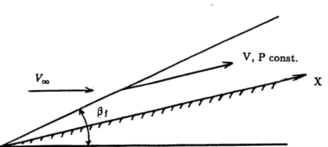
This thesis considers only the attenuation of the electromagnetic waves propa-gating in the z-direction which is perpendicular to the wedge surface, as shown in

Electromagnetic

Figure 4.1: Schematic of Electromagnetic Wave Propagation over a Wedge

Fig. 4.1. This propagation path is considered to be the most desirable for communi-cations since it minimizes the path length to the antenna.

Since the angle between the shock and the wedge (Pj - 0) is small, a few degrees

at most, the direction of propagation is almost perpendicular to the shock. Since the flow properties in the inviscid region change only in the direction perpendicular to the shock, from the assumption in the previous chapter, the plasma properties are varying only in the direction of propagation. It is also assumed that, in the boundary layer, the local variation of the plasma properties in the z-direction is negligible compared with that in the z-direction. In this case, E and VKp are orthogonal and Eq.(4.20) becomes

--

+

If the value of Kp varies only slightly over the length of the electromagnetic wave,

then the approximate solution of Eq.(4.22) is given by an expression of the form:

-=

(4.23)

A = kfRe( V )dz

B = k Im(R)dz

=

f

dz

(4.25)

2

and any reflected wave has been neglected. Since most of the attenuation is expected in the boundary layer, the thickness of which is of the order of centimeter, Eq.(4.23)

will give a good approximation for electromagnetic waves with a wave length which

is less than that order.

Since the electromagnetic wave is attenuated due to the term of e- A_{, and K,}

in this term is a function of wp and vyff, these values need to be given along the propagation path. w, is a function of electron density only as shown in Eq.(4.15).

vfy is evaluated by the following expressions(Appendix C)in this work:

Veff = Veff,m + Veff,i

Veffm - 4a 2Un (4.26) 3 Veff,i = 7r (T)2 vn i In 0.37 (4.27) .T e2n 3 where

= (=8,T)

(4.28)

r. is the Boltzmann constant, a is the radius of molecules, and n, and ni are the number densities of molecules and electrons, respectively.

Chapter 5

Numerical Results

This chapter presents the numerical results of the flow properties over a wedge and the attenuation of the electromagnetic waves propagating through the flow. The

parameters considered in the calculations are shown in Table 5.1.

5.1

Flow Results

This section shows the chemical composition in the flow over a wedge. The flow field is divided into two regions:the inviscid region and the boundary layer. In the

inviscid region, the finite rate chemistry is considered. The boundary layer is assumed to be laminar and in equilibrium.

5.1.1

Inviscid Region

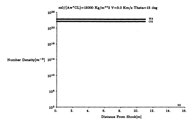
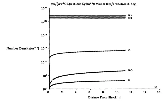
The species distributions behind an oblique shock for various free stream velocities

along the middle trajectory are shown in Figs 5.1- 5.5. The wedge angle 0 is 15 degrees for all the cases.

As the velocity increases,the dissociation of oxygen is first observed at V=4 Km/s (M=13.1). The production of electrons becomes noticeable at V=6.5 Km/s

(M=19.7), and at V=7.5 Km/s (M=24.7), the number density of electrons reaches

Table 5.1: Calculation parameters

trajectory wedge angle[deg] wall temperature[K] velocity[Km/s]

upper 15 1500 2 -- 7.5 10 1500 2 ---+ 7.5 1000 2 --+ 7.5 middle 15 1500 2 --- 7.5 2000 2 --+ 7.5 20 1500 2 -- + 7.5 lower 15 1500 2 -- + 7.5

Figure 5.6 shows the effect of trajectory on the species concentrations for V=6.5 Km/s, 0 = 15 degrees, and Tw = 1500K. As the altitude becomes lower, the concentration of electrons increases.

Figure 5.7 shows the effect of wedge angle for V=6.5 km/s in the middle trajectory.

The electron concentration increases significantly with the increase in wedge angle.

For 0 = 20 degrees, the number density of electrons increases rapidly within a few meters from the shock and reaches the order of 10'1m - 3 _{approximately 7 m from the}

m0/(Aw*CL)=15000 Kg/m**2 V=3.0 Km/s Theta=15 deg 10 y 1022. 101 i Number Density[m- a] 1014 -1010 106 102 0. 2. 4. 6. 8. 10. 12. 14. 16.

Distance From Shocklml

Figure 5.1: Nonequilibrium species distributions behind a shock at V=3.0 Km/s

106. 1022 Number Density[m- 3 10W14 1010o 106 102 0

mO/(Aw*CL)=15000 Kg/m**2 V=4.0 Km/s Theta=15 deg

N2

02

2. 4. 6. 8. 10. 12. 14. 16.

Distance From Shock[m]

Figure 5.2: Nonequilibrium species distributions behind a shock at V=4.0 Km/s 12A

--10" 1022 1018 . Number Density(m-31 1014 101o0. 106

-in2

m0/(Aw*CL)=15000 Kg/m**2 V=5.0 Km/s Theta=15 deg

N2 02

I I

I

Figure 5.3: Nonequilibrium species distributions behind a shock at V=5.0 Km/s

mO/(Aw*CL)=15000 Kg/m**2 V=6.5 Km/s Theta=15 deg 10·'~ 10AA 1018 Number Density[m-3] 1014. 100. 106 in2 0. 2. 4. 6. 8. 10.

Distance From Shock[m]

Figure 5.4: Nonequilibrium species distributions behind a shock at V=6.5 Km/s

12. 14. 16. N2 02 . NO+ 02+ 14. 16. . . ,LIIII ** 2. 4. 6. 8. 10.

Distnce From Shock[m)

...

/S=r=LZr

~c~-cl---~----~

m0/(Aw*CL)=15000 Kg/m**2 V=7.5 Km/s Theta=15 deg 1026 1022 Number Density[m- 3 ] 1014 1010 106 102

Figure 5.5: Nonequilibrium species distributions behind a shock at V=7.5 Km/s

0 NO N e NO+ 02+ 0. 2. 4. 6. 8. 10. 12. 14. 16.

Distance From Shock[m]

1

-Number Density[m- 3 ] Number Density[m-3 ] Number Density[m- 8 ]

m0/(Aw*CL)=5000 Kg/m**2 V=6.5 Km/s Theta=15 deg 1026 N2 1022 02 10ts 0 1014 NO 1010 106 upper trajectory 102 0. 2. 4. 6. 8. 10. 12. 14. 16. Distance From Shock(m]

mO/(Aw*CL)=15000 Kg/m**2 V=6.5 Km/s Theta=15 deg 1026 1022 1014 106 102 . 0 1026 1022 1018 1014 1010 106 102 0 i- 0 .-~---c NO II I I I .. ~---II middle trajectory e NO+ 02+ 2. 4. 6. 8. 10. 12. 14. 16. Distance From Shock(m]

m0/(Aw*CL)=25000 Kg/m**2 V=6.5 Km/s Theta=15 deg

N2 o2 NO N I. lower trajectory e NO+ 02+ 2. 4. 6. 8. 10. 12. 14. 16.

Distance From Shock[m]

Figure 5.6: Effect of trajectory on nonequilibrium species distributions behind a shock at V=6.5 Km/s

mO/(Aw*CL)=15000 Kg/m**2 V=6.5 Km/s Theta=10 deg Number Density[m- SJ Number Density[m- 3 ] Number Density[m- 3 ] 1026 1022 101. 1014 1010o 106 mn2 0. 1026 1022 101' 1014 1010 106 102 0. 102 1022 1018 1014 1010 106 102 0. 0 Theta= 1 deg 2. 4. 6. 8. 10. 12. 14. 16. Distance From Shock[m]

mO/(Aw*CL)=15000 Kg/m**2 V=6.5 Km/s Theta=15 deg

N2 02 Theta=15 deg e NO+ 02+ 2. 4. 6. 8. 10. 12. 14. 16. Distance From Shock[m]

m0/(Aw*CL)=15000 Kg/m**2 V=6.5 Km/s Theta=20 deg

N e0 ~o2 2. NO+ I+ o+ N2+ N+ Theta=20 deg 4. 6. 8. 10. 12. 14. 16. Distance From Shock[m)

Figure 5.7: Effect of wedge angle on nonequilibrium species distributions behind a shock at V=6.5 Km/s I LIIIIII t m * /L~-~·LLIICC--

~---5.1.2

Boundary Layer

The velocity profiles, the temperature profiles, and the concentrations in the

boundary layer 10 m downstream from the leading edge for various free stream

ve-locities along the middle trajectory are shown in Figs 5.8- 5.17. The wedge angle and wall temperature are 8 = 15 degrees and Tw = 1500 K, respectively.

The boundary layer thickness increases with velocity from about 1 cm at V=3.0

Km(M=10.0) to about 8 cm at V=7.5 Km/s(M=24.7). The maximum number

den-sity of electrons reaches the order of 10'1m-S at V=5.0 Km/s, and beyond that

velocity, it does not increase significantly because of the rapid decrease of the air

density along the trajectory. The region with high electron density,however, increases

m0/(Aw*CL)=15000 Kg/m**2 V=3.0 Km/s Theta=15 deg Tw=1500 K 1.250 1.000 Y[m] 0.500 0.250 TIKI U[m/l) 0.0 1.0 2.0 3.0 4.0 5.0 Velocity[m/s], Temperature(K] Figure 5.8: 6.0 7.0 8.0 x 103

Velocity and temperature profiles in a boundary layer at V=3.0 Km/s

mO/(Aw*CL)=15000 Kg/m**2 V=3.0 Km/s Theta=15 deg Tw=1500 K

1.250 1.000 Y[m] 0.500 0.250 No O2 N2 1022 1024 1026

Figure 5.9: Species concentrations in a boundary layer at V=3.0 Km/s

101o0 1012 1014 1016 101 1020 Number Density fm-3] _ _^_

m0/(Aw*CL)=15000 Kg/m**2 V=4.0 Km/s Theta=15 deg Tw=1500 K 1.250 1.000 0.500 0.250 TI[K Ulml/. 0.0 1.0 2.0 3.0 4.0 5.0 Velocity[m/s), Temperature[K] Figure 5.10: Y[m] 6.0 7.0 8.0 x 103

Velocity and temperature profiles in a boundary layer at V=4.0 Km/s m0/(Aw*CL)=15000 Kg/m**2 V=4.0 Km/s Theta=15 deg Tw=1500 K

1022 1024 1026

Figure 5.11: Species concentrations in a boundary layer at V=4.0 Km/s

1010 1012 1014 1016 10o I 1020 Number Density [m-31 t F#%•i

m0/(Aw*CL)=15000 Kg/m**2 V=5.0 Km/s Theta=15 deg Tw=1500 K 2.50 2.00 Y(m] 1.00 0.50 T[KI U['m/, 0.0 1.0 2.0 3.0 4.0 5.0 Velocity[m/a], Temperature[(K 6.0 7.0 8.0 x 103

Figure 5.12: Velocity and temperature profiles in a boundary layer at V=5.0 Km/s

m0/(Aw*CL)=15000 Kg/m**2 V=5.0 Km/s Theta=15 deg Tw=1500 K

2.50 2.00 Y[m) 1.00 0.50 O NO 02 N2 1022 1024 1026

Figure 5.13: Species concentrations in a boundary layer at V=5.0 Km/s 1010 1012 10" 1016 1018 1020

Number Density [m- 3 ]

mO/(Aw*CL)=15000 Kg/m**2 V=6.5 Km/s Theta=15 deg Tw=1500 K

TIKI Ulm/sl

1.0 2.0 3.0 4.0 5.0 6.0 7.0 8.0 x 103

Velocity(m/s], Temperature(K]

Figure 5.14: Velocity and temperature profiles in a boundary layer at V=6.5 Km/s

m0/(Aw*CL)=15000 Kg/m**2 V=6.5 Km/s Theta=15 deg Tw=1500 K

Y[m]

1010 1012 ' 101 1016 1020 1022 1024 1026

Number Density m-3

Figure 5.15: Species concentrations in a boundary layer at V=6.5 Km/s

2.50 2.00 Y[m] 1.00 0.50 0.0 a f%

m0/(Aw*CL)=15000 Kg/m**2 V=7.5 Km/s Theta=15 deg Tw=1500 K T(K] 0.0 1.0 2.0 3.0 4.0 5.0 Velocity[m/s), Temperature(KI Ulm/al 6.0 7.0 8.0 x 103

Velocity and temperature profiles in a boundary layer at V=7.5 Km/s

m0/(Aw*CL)=15000 Kg/m**2 V=7.5 Km/s Theta=15 deg Tw=1500 K

e NO+ NOO 02 N2

102 1014 101'6 108 1020 Number Density [m- 3

]

1022 1024 1026

Figure 5.17: Species concentrations in a boundary layer at V=7.5 Km/s

Y(m) Figure 5.16: 0.12 0.10 0.08 Y[m] 0.06 0.04 0.02 0.00 1010 02+

Figure 5.18 shows the effect of trajectory on the velocity and temperature profiles

in a boundary layer at V=6.5 Km(M=19.7) for the wedge angle 0 = 150 and the wall temperature Tw = 1500 K. Figure 5.19 shows the effect of trajectory on the

concentrations in a boundary layer for the same conditions. As the altitude decreases, the boundary layer thickness decreases and the maximum electron density increases. Figure 5.20 shows the effect of wedge angle on the velocity and temperature profiles in a boundary layer at V=6.5 Km(M=19.7) in the middle trajectory for

Tw = 1500K. Figure 5.21 shows the effect of wedge angle on the concentrations in a boundary layer for the same conditions. As the wedge angle increases, the boundary layer thickness decreases and the electron density increases significantly.

Figure 5.22 shows the effect of wall temperature on the velocity and temperature

profiles in a boundary layer at V=6.5 Km(M=19.7) in the middle trajectory for

0 = 15'. Figure 5.23 shows the effect of wall temperature on the concentrations for

the same conditions. The variation of the boundary layer thickness with the wall

temperature is very small for the range 1000K < Tw < 2000K. The increase of the electron density with the increase in wall temperature is noticeable only in the

m0/(Aw*CL)=15000 Kg/m**2 V=6.5 Km/s Theta=15 deg Tw=1500 K

T(K] Ulm/s]

rajectory

D x 10* Velocity[m/s], Temperature[K]

m0/(Aw*CL)=15000 Kg/m**2 V=6.5 Km/s Theta=15 deg Tw=1500 K

Y[( ,0. 6.0 x 10- 2 5.0 4.0 Y[mj 3.0 2.0 1.01 0n T[KJ U[m/,j trajectory 0 1.0 2.0 3.0 4.0 5.0 6.0 7.0 8.0 Velocity[m/sJ, Temperature[K] m0/(Aw*CL)=25000 Kg/m**2 V=6.5 KM/s Theta=15 T[K) U[m/sJ lower tr 0.0 1.0 2.0 3.0 4.0 5.0 6.0 7.0 8.( Velocity(m/s], Temperature[K] x 103 deg Tw=1500 K ajectory S x 103

Figure 5.18: Effect of trajectory on Velocity and temperature profiles in a boundary layer at V=6.5 Km/s

m0/(Aw*CL)=5K00 Kg/m**2 V=6.5 Km/s Theta=15 deg Tw=1500 K

xl

Y(m]

Number Density [m- 8

]

m0/(Aw*CL)=15000 Kg/m**2 V=6.5 Km/s Theta=15 deg Tw=1500 K

e NO+ N 02+ ON002N2

S

middle

trajectory

m0/(Aw*CL)=25000 Kg/m**2 V=6.5 Km/s Theta=15 deg Tw=1500 K

e NO+ N ONO 02N2 oN2+ 2+ lower tr 010o 1012 1014 1016 10'5 1020 102 104 102 Number Density [m- _1j ajectory 6

Figure 5.19: Effect of trajectory on concentrations in a boundary layer at V=6.5 Km/s rajectory 26 6.0 x 10 -5.0 4.0 Y[m] 3.0, 2.0 1.0 nn. 6.0 x 10- 2 5.0. 4.0 Y[m] 3.0. 2.0 1.0 0. 0 •A - --

----m0/(Aw*CL)=15000 Kg/m**2 V=6.5 Km/s Theta=10 deg Tw=1500 K T[KI le 0 X 103 Velocity[m/s], Temperature[K) m0/(Aw*CL)=15000 Kg/m**2 V=6.5 Km/s Theta=1500 K Tw=1500 K Y[n 0.b Y[m] leg 0 1.0 2.0 3.0 4.0 5.0 6.0 7.0 8.0 x 103 Velocity(m/sj, Temperature(K]

m0/(Aw*CL)=15000 Kg/m**2 V=6.5 Km/s Theta=20 deg Tw=1500 K

TIKJ

eg

0.0 1.0 2.0 3.0 4.0 5.0 6.0 7.0 8.0 x 103 Velocity[m/s], Temperature[K]

Figure 5.20: Effect of wedge angle on Velocity and temperature profiles in a boundary layer at V=6.5 Km/s

x1

Y[mI

m0/(Aw*CL)=15000 Kg/m**2 V=6.5 Km/s Theta=10 deg Tw=1500 K

1012 1014 1016 101' 1020 1022 1024 10i

Number Density [m- ] 1

mO/(Aw*CL)=15000 Kg/m**2 V=6.5 Km/s Theta=15 deg Tw=1500 K 6.0-x 10- 2 5.0' 4.0 Y[m) 3.0 0.0

N

m0/(Aw*CL)=15000 Kg/m**2 V=6.5 Km/s Theta=20 deg Tw=1500 K

eNO+ N NO N2

0 = 20deg

1014 1016 10I' 1020 1022 1024 1026

Number Density [m-3a

Figure 5.21: Effect of wedge angle on concentrations in a boundary layer at V=6.5

Km/s Y[n 5.0 4.0 Y[m] 3.0 20n n0 02+ 1010 1012 _ _

a#

ii

m0/(Aw*CL)=15000 Kg/m**2 V=6.5 Km/s Theta=1500 deg Tw=1000 K

OOOK

0 1.0 2.0 3.0 4.0 5.0 6.0 7.0 8.0 x 103 Velocity[m/s], Temperature(K]

m0/(Aw*CL)=15000 Kg/m**2 V=6.5 Km/s Theta=15 deg Tw=1500 K

S00K 0 1.0 2.0 3.0 4.0 5.0 6.0 7.0 8.0 Velocity[m/s], Temperature[K] m0/(Aw*CL)=15000 Kg/m**2 V=6.5 Km/s Theta=15 x 103 deg Tw=2000 K 000K S 10'3 Velocity[m/s], Temperature[K)

Figure 5.22: Effect of wall temperature on Velocity and temperature profiles in a boundary layer at V=6.5 Km/s x Y[m] 0.( X Y[mJ 0.C x Y[rn] • M

mO/(Aw*CL)=15000 Kg/m**2 V=3.0Km/s Theta=15 deg Tw=1500 k X=10 m

DO K

10o 10' 10 101 10 10'6 10 101 102 1022 1024 1026

Number Density [m-a]

m0/(Aw*CL)=1500 Kg/m**2 V=6.5 Km/s Theta=15 deg Tw=1500 K

600K

101o0 1012 1014 1016 101" 1020 1022 1024 1026

Number Density [m-8 ]

mO/(Aw*CL)=15000 Kg/m**2 V=6.5 Km/s Theta=15 deg Tw=2000 K

Y[m

000K

101o 1012 1014 10'6 10I s 1020 102 1024 1026

Number Density [m

-3]

Figure 5.23: Effect of wall temperature on concentrations in a boundary layer at V=6.5 Km/s

x

Y(m]

5.2

Attenuation of Electromagnetic Waves

This section presents the numerical results of the attenuation of the power of the

electromagnetic waves propagating through the plasma over a wedge. The location

of antenna is tentatively chosen to be 10 m from the leading edge.

Figure 5.24 shows the effect of trajectory on the attenuation for 8 = 150 and

Tw = 1500K. In this figure, the attenuation is shown with the frequency of the electromagnetic waves for various velocities. The attenuation becomes significant

above V=5.0 Km/s(M=16.0) for all the trajectories below some frequency, which increases with decreasing altitude. This critical frequency is 2.4 GHz for the upper, 4 GHz for the middle, and 6.3 GHz for the lower trajectory. The magnitude of

attenuation becomes 3 dB at about V=6.5 Km/s(M=20) and reaches about 10 dB

at V=7.5 Km/s(M=25) for 1 GHz. This result shows that electromagnetic waves

with radio frequencies in S band(2-4 GHz) or lower are strongly attenuated along the upper trajectory and those in C band(4-6 GHz) or lower are attenuated along

the middle and lower trajectories. On the other hand, no noticeable attenuation is

observed in X band(8-12 GHz).

Figure 5.25 shows the effect of wedge angle on the attenuation along the middle

trajectory for Tw = 1500K. The attenuation increases significantly with the increase in wedge angle and the critical frequency increases from 2.4 GHz for 0 = 100 to 10

GHz for 0 = 20*. This result shows that for 0 = 20*, communications with X band are also attenuated at high velocities. The drastic increase of the attenuation with

increased wedge angle corresponds to the rapid increase of the electron density in the inviscid region and the outer part of the boundary layer. On the other hand, the critical velocity above which the attenuation becomes significant does not change considerably with wedge angle.

Figure 5.26 shows the effect of wall temperature on the attenuation along the middle trajectory for 0 = 15*. The attenuation for each velocity increases with increased wall temperature; however, the critical frequency is relatively constant.