Economic Analysis of Shale Gas Wells in the United States
byChristopher D. Hammond
Submitted to the
Department of Mechanical Engineering
In Partial Fulfillment of the Requirements for the Degree of Bachelor of Science in Mechanical Engineering
ARCHP&c,
at theF F TECMT Massachusetts Institute of Technology
June 2013 L
LiBAR
Es
0 2013 Christopher D. Hammond All rights reserved
The author hereby grants to MIT permission to reproduce and to distribute publicly paper and electronic copies of this thesis document in whole or in part in any medium now
known or hereafter created.
Signature of Author
Department of Mechanical Engineering May 10, 2013
Certified by
Francis O'Sullivan Executive Director, Energy Sustainability Challenge, MIT Energy Initiative Thesis Supervisor
Accepted by
Annette Hosoi Professor of Mechanical Engineering Undergraduate Officer
Economic Analysis of Shale Gas Wells in the United States
by
Christopher D. Hammond
Submitted to the Department of Mechanical Engineering on May 10, 2013 in Partial Fulfillment of the
Requirements for the Degree of
Bachelor of Science in Mechanical Engineering
ABSTRACT
Natural gas produced from shale formations has increased dramatically in the past decade and has altered the oil and gas industry greatly. The use of horizontal drilling and hydraulic fracturing has enabled the production of a natural gas resource that was previously unrecoverable. Estimates of the size of the resource indicate that shale gas has the potential to supply decades of domestically produced natural gas. Yet there are challenges surrounding the production of shale gas that have not yet been solved. The economic viability of the shale gas resources has recently come into question. This study uses a discounted cash flow economic model to evaluate the breakeven price of natural gas wells drilled in 7 major U.S. shale formations from 2005 to 2012. The breakeven price is the wellhead gas price that produces a 10% internal rate of return.
The results of the economic analysis break down the breakeven gas price by year and shale play, along with P20 and P80 gas prices to illustrate the variability present. Derived vintage supply curves illustrate the volume of natural gas that was produced economically for a range of breakeven prices. Historic Natural Gas Futures Prices are used as a metric to determine the volumes and percentage of total yearly production that was produced at or below the Futures Price of each vintage year. From 2005 to 2008, the total production of shale gas resulted in a net profit for operators. A drop in price in 2009 resulted in a net loss for producers from 2009 to 2012. In 2012, only 26.5% of the total gas volume produced was produced at or below the 2012 Natural Gas Futures Price.
Thesis Supervisor: Francis O'Sullivan
Table of Contents Abstract 3 Table of Contents 4 List of Figures 6 List of Tables 7 1. Introduction 8
1.1 What is Shale Gas? 9
1.2 Enabling Technology 10
1.3 Environmental Risks 14
1.4 The Rise of Shale Gas 17
1.5 Historic Natural Gas Economics 23
1.6 Implications of Shale Gas Production 24
2. Current Situation and Challenges 26
2.1 Supply Increase, Price Decrease 26
2.2 Production Variability 27
3. Method for Economic Analysis 29
3.1 Revenue Streams in the Economic Model 31
3.1.1 Decline Curves and EUR 31
3.1.2 Determining the Correct LGR Calculation 34
3.1.3 Natural Gas Liquids Pricing 35
3.2 Costs in the Economic Model 36
3.3 MATLAB Calculation and Optimization Scheme 38
4. Results 40
4.1 Breakeven Price Distribution 40
4.2 Supply Curves 42
4.2.1 The Shift to Liquids-Rich Areas 44
4.2.2 Past Breakeven Volumes and Percentages 45
4.3 Aggregate Vintage Shale Gas Profitability 46
5. Discussion and Implications of Analysis 49
5.1 Will production decline? 49
5.3 Beneficiaries of Low-Price Gas 51
5.4 International Implications 51
5.5 Criticisms of Analysis Method 53
6. Conclusion 54
7. Appendices 57
Appendix A: Breakeven Price Cumulative Distribution Functions by Play 57
Appendix B: United States Vintage Supply Curves 64
List of Figures
Figure 1-1: Schematic geology of natural gas resource 9
Figure 1-2: Typical casing and cement program 11
Figure 1-3: Effects of stresses, wellbore orientation on fracture propagation 13
Figure 1-4: Map of shale plays in the lower 48 United States 18
Figure 1-5: Contributions to total U.S. shale gas production 18
Figure 1-6: EIA U.S. natural gas production projections 19
Figure 1-7: Historic U.S. natural gas wellhead prices 24
Figure 2-1: Distribution of Barnett peak gas production rates 28
Figure 3-1: Normalized production decline curves of select Barnett vintages 32
Figure 3-2: CDF of 2006 vintage Bamett LGRs calculated with 3 different data sets 35
Figure 4-1: CDF of breakeven prices for Barnett vintages 40
Figure 4-2: U.S. shale gas vintage supply curves 43
Figure 4-3: Select U.S. supply curves highlighting shift to liquids-rich areas 45 Figure 4-4: Supply curve representation of value captured, loss, and revenue 47
List of Tables
Table 1-1: Summary of shale gas resources for 32 countries 22
Table 2-1: Barnett well peak production rate statistics 28
Table 3-1: Number of wells analyzed by play and year 31
Table 3-2: Arps decline curve parameters for select Barnett wells 33
Table 3-3: Barnett shale tax write down schedule 37
Table 3-4: Summary of economic model input values 39
Table 4-1: Summary of P20, P50, P80 breakeven prices for all wells 41
Table 4-2: Past breakeven volumes, percentages of vintage total production 46 Table 4-3: Revenue, costs, and net profit/loss for U.S. vintage shale gas 48
1. Introduction
In recent years, the rapid increase in natural gas production from shale formations has had a major impact on the oil and gas industry in North America. Within the span of a decade, the rise of natural gas production from shale rocks has opened up vast natural gas resources that were previously unrecoverable. In addition, countries all over the world are paying close attention to natural gas production in the United States and considering producing natural gas from shale formations in their own countries. Despite these recent advances, there are considerable challenges that remain unsolved in the production of these unconventional resources. One prominent issue is the variability of productivity from well-to-well, even within the same shale formation, which gives rise to further challenges. For one thing, it becomes very difficult to accurately assess the amount of natural gas that can be recovered from shale formations. This poses problems for a range of stakeholders, from production companies to those trading natural gas and land resources.
This study uses an economic model and historic individual well production data to deduce a breakeven price of natural gas for each well. Aggregating these individual breakeven gas prices with corresponding gas volumes produces supply curves that show what quantities of natural gas were economically viable at various natural gas prices. Since the supply curves are derived from individual well breakeven prices, unique supply curves can be created based on different combinations of years and shale formations. In total, this study examines horizontally drilled natural gas wells from the past eight years across seven major U.S. shale gas plays. Results highlight historical trends in the
economic viability of natural gas produced from shale rock formations. Most notably, as natural gas supplies rose and price dropped, producers moved to areas of shale formations that produced natural gas liquids as well as natural gas. This phenomenon has resulted in significant quantities of natural gas with a break-even price of zero dollars, which has a broad range of implications from affecting future gas prices to impacting the chemical and energy sectors. Additionally, the vintage supply curve of any given year analyzed can be compared to the natural gas price of that year to make an assertion about what volume of gas resulted in a profit for the producing companies and what volume resulted in a loss.
1.1 What is shale gas?
Natural gas, like crude oil, is formed from organic matter that becomes buried and is transformed over thousands of years under immense heat and pressure. As such, natural gas and crude oil are found deep within the earth's crust in reservoirs at high pressures. Natural gas can be found with or without crude oil, in a variety of reservoir types as Figure 1-1 illustrates below. Natural gas that is found in a reservoir also
containing oil is called associated gas, while natural gas that is found without oil is called non-associated gas. Both associated gas and non-associated gas fall under the category of conventional gas resources. Conventional resources develop when organic material is turned into hydrocarbons like oil and gas in a permeable source rock. The oil and gas then migrates towards the surface until it reaches a layer of rock that is impermeable. The oil and gas collect under the impermeable layer, held in place by a buoyant force, in a permeable rock termed the reservoir rock. Conventional resources are extracted by drilling into the reservoir rock, which allows the high pressure within the rock to push the gas and/or oil to the surface where it is collected.
Co- bed 0*n.
Unconventional resources are found in rocks where the permeability is extremely low, so gas cannot migrate to another formation. Instead, small droplets of gas or oil are trapped within pores in the rock. One type of rock in which unconventional resources are often found is shale. The shale serves as both the source and reservoir rock in these cases. This study focuses on natural gas found in shale formations. Shales have a permeability that is on the order of 0.01 to 0.00001 millidarcies. A darcy is a unit of permeability. A medium that has a permeability of 1 darcy allows a fluid with a viscosity of I mPa*s to have a volumetric flow of 1 cm 3/s under a pressure gradient of 1 atm/cm
acting across a 1 cm2 area. The extremely low permeability of shale means that extracting natural gas from shale formations requires the use of distinct technologies. Hydraulic fracturing is a process that creates pathways within the shale formation to allow natural gas to flow out of the rock. The specifics regarding this technology will be discussed in the next section.
1.2 Enabling Technology
The technologies that have unlocked the expansive and previously unrecoverable shale gas and shale oil resources, horizontal drilling and hydraulic fracturing, are not new technologies as is often thought. For decades, production companies have used
horizontal drilling and hydraulic fracturing to increase the production of conventional resources. However, in the past decade the novel use of these two technologies in combination has become widespread and allowed vast resources locked in shale
formations to be recovered. The use of hydraulic fracturing to extract natural gas and oil from shale rocks is not without controversy. Environmental concerns arise at many stages of production and are widely publicized. These concerns will be addressed briefly following an explanation of horizontal drilling and hydraulic fracturing, but the purpose of this study is not to analyze the environmental effects of shale gas production. This study assumes that with proper regulation and responsible practices, shale gas production can and will continue into the future in an environmentally friendly way.
Before operators can drill land, they are required to obtain a permit to drill from the state in which they are drilling. Then, the first step in production of natural gas from
drilling is that it greatly increases the contact area between the wellbore and the rock formation in comparison to conventional drilling, which is done vertically. To begin, a production company drills vertically down into the earth to different depths before cementing a steel tube in place to keep the well open. Typically three layers of cement and steel casing are set in place to different depths before the final production casing is run to bottom of the well. The purpose of the cement and steel casing are to separate the
layers of rock and ground water above the shale formation from the shale formation itself. Figure 1-2, below, shows a representation of a typical casing and cement program. This process is not a perfect one and has led to shale gas development coming under fire for environmental issues related to groundwater contamination.
- Conductor Casing 100
-1000
-I
2000 - Salt Water Zone7100 - Kickoff Point I:II-iICement Surface Casing Drilling Mud ~---Intermediate Casing --- Cement Production Casing Production Tubing
ALL LOnSUMQ OUU5
Figure 1-2: Schematic of typical casing and cement program
Not to Scale
The wellbore is drilled vertically until it is just above the top of the shale formation. At this point, a specialized drill bit is used to turn the well at a rate of a few
degrees per hundred feet until it has made a 90-degree turn and runs horizontally through the shale formation. The direction of the wellbore through the shale formation is
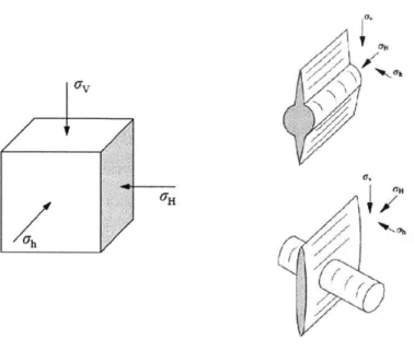
important for hydraulic fracturing. The wellbore is aligned parallel to the direction of the least compressive stress within the shale formation. Shale formations fracture in an orientation that is perpendicular to the direction of least compressive stress because the least compressive stress is the first to be overcome, resulting in the fracturing of the rock. This means that the wellbore is perpendicular to the dominant orientation of fractures in a formation where fractures are naturally occurring [I]. A prominent benefit of horizontal drilling is the ability to drill multiple wells from a single well pad, sometimes called "pad drilling". Drilling pads are usually 3-5 acres in size, and one drill pad is typically used to drill approximately 6 wells. Pad drilling greatly reduces the time, cost, and
environmental impact of drilling shale gas wells.
After the well has been drilled into the shale formation, it is ready to be hydraulically fractured. Before hydraulic fracturing, or fracking, can be done the
wellbore is perforated at specific points along the horizontal section to open the bottom of the wellbore to the rock formation. In shale formations, the low permeability prevents gas from migrating. Hydraulic fracturing is the process of creating pathways in the shale for the gas to flow out. Large volumes of fluid containing roughly 99% water and sand and 1% chemicals, are pumped into the well at high pressures. This is where the direction of the wellbore within the formation becomes important. Figure 1-3 illustrates the effect of wellbore orientation on fracture propagation. The graphic in the bottom right of Figure 1-3 shows the case where the wellbore is oriented parallel to the minimum horizontal compressive stress (or conversely, perpendicular to the maximum horizontal stress). The high pressure overcomes the least compressive stress within the shale rock, opening fractures that extend dominantly in the direction perpendicular to the wellbore. This is repeated at several locations or "stages" along the wellbore, creating a large network of fractures in the shale formation that are open to the wellbore. The sand in the fracking fluid keeps the cracks in the shale open so that gas can flow for years, and the chemicals mainly lower surface tension to help increase the flow of natural gas to the surface.
1V '7H 17~ /1 p7 -/ **I~Ka, ~, N / N N > / // (7 1-~/~~
Figure 1-3: Effects of horizontal stresses, wellbore orientation on fracture propagation
The best shales for hydraulic fracturing are those that fracture in a brittle, rather than ductile, manner. Ductile shales tend to resist fracturing and deform intemally, while
brittle shales fracture more easily and respond well to the hydraulic fracturing process [1]. Shale gas wells tend to have a steep decline in production rate during the first year. This decline is typically about a 60% drop-off after one year and is relatively consistent in past years across shale formations. Though sophisticated seismic techniques are used to estimate the characteristics of hydraulically induced fractures, the models are not exact. For this reason and others, the production rates of natural gas wells can vary unpredictably, as will be discussed later. The development of both micro and macro scale seismic techniques could help improve the accuracy and productivity of fracking operations.
Another important technical aspect of natural gas found in shale rock formations is that not all areas produce the exact same mixture of gas and liquids, even within the
same play. Natural gas is primarily composed of methane, which is the simplest and lightest possible hydrocarbon molecule consisting of four hydrogen atoms attached to a
single carbon atom (CH4). However, the geological process that turns organic matter into
natural gas can lead natural gas in shale formations to contain smaller amounts of heavier hydrocarbons such as ethane (C2H6), propane (C3H8) and butane (C4H10) [2]. These
heavier hydrocarbons are produced from the shale rock formation along with methane and are referred to as natural gas liquids (NGLs). Natural gas liquids are sold at a separate, higher price than natural gas which in many cases can help offset the cost of producing and selling natural gas at a low gas price, making a particular area within a shale play more lucrative. Areas that tend to produce relatively high amounts of NGLs are called liquids-rich. A ratio called the liquid-to-gas ratio is used in the industry to quantify how liquids-rich a particular area is. The ratio is just as it sounds, a ratio of barrels of oil equivalent liquids to million cubic feet of gas (boe/MMcf). The fact that NGLs fetch a considerably higher price than natural gas makes liquids-rich areas of shale plays desirable.
1.3 Environmental Risks
Though the use of horizontal drilling and hydraulic fracturing has rapidly
increased in recent years, the technologies do come with environmental risks. There are even some who claim that shale gas production is currently causing considerable
environmental damage. Though hydraulic fracturing is most often the process attacked as environmentally damaging because of its use of chemicals and massive volumes of water, the process of horizontal drilling is not without its own set of environmental concerns. Multiple environmental risks surround the issue of water. One issue is quite plainly the enormous amount of water that is used in each fracking operation. It is typical for a fracking operation to consume from 2 to 4 million gallons of water for a single well.
Standing alone, this is a massive amount of water, but studies have shown that it is just a small portion of the water consumption in areas where shale gas is developed. Water use
by shale gas ranges from less than 0.1% to 0.8% of total water use in the area of the shale
play, substantially outpaced by use for livestock, irrigation, industrial/mining, and public supply [3]. Regardless, shale gas producers are continuing to improve in reusing fracking
fluid that returns from the well in order to reduce overall water use. Another issue surrounding water is the occurrence of surface spills at a drilling or fracking site. There are many fluids used in the production of shale gas, with the most common being drilling mud and fracking fluid. Surface spills can occur as a result of equipment failure like pumps and hoses, or as a result of overflow of a tank or surface pit. If a large volume of fluid is spilled it could contaminate local waterways and cause further problems. A third water related environmental risk is the disposal of flow-back fluid, which is a mix of fracking fluid and formation water that is returned back up the well after the completion of a fracking operation but before production. The flow-back fluid typically has high salinity and can contain naturally occurring radioactive material (NORM) from deep within the ground. In some states the practice is to inject the flow-back fluid into an EPA regulated disposal well, while in others like Pennsylvania the fluid is taken to waste treatment plants, many of which cannot handle the high contamination levels of the flow-back fluid. The issue of disposal of flow-flow-back fluid is an ongoing problem.
Other environmental impacts affect the communities in the shale play area more directly. Many of the shale gas plays are located in rural areas where the residents rely on the groundwater table as their supply of potable water. The most common cause of reported environmental incidents is the migration of natural gas or drilling fluids into groundwater zones, which is related to issues that occur while drilling and setting the casing that is supposed to protect the groundwater. There are a few causes for this contamination. One cause could be that the drilling fluid, or "drilling mud," is too dense and therefore pressure at the depth of the groundwater table causes the drilling mud to move into the groundwater table. Another cause could be that the wellbore enters an unexpected pocket of natural gas, and the open passageway to the groundwater table results in natural gas migrating to and contaminating the groundwater. Lastly, if the casing that protects the groundwater is poorly cemented in place it could result in an open pathway to the groundwater table by which contaminants from subsequent operations could migrate into the groundwater. Regardless of the source of contamination, if the groundwater table becomes unfit for use in an area that depends on it for its water supply, the community is greatly affected. Production companies that caused groundwater contamination in the past have had to pay to have potable water shipped to rural
residents. Another way the community and local environment are affected by shale gas production is the large increase in traffic and infrastructure in the areas of drilling. Many
drilling locations are inaccessible by roads, so the production company must build a road in order to transport the rig and supplies to the location. Estimates for the number of truck trips to a shale well site for both drilling and completion range from 890 for drilling
and completing one well to 8,900 for two drilling rigs and completion supplies for 8 wells [3]. For the rural communities of many shale gas plays, this large increase in truck traffic disrupts their way of life. Additionally, the construction of access roads and well pads causes damage to the community and local environment.
A controversial but nonetheless important environmental concern surrounding shale gas development is the issue of harmful air emissions. It is recognized that engines for drilling rigs, pumps, mixers, trucks, and similar equipment that run on a hydrocarbon fuel will produce some level of harmful air emissions. However, these emissions are known and essentially taken as a given in the process of natural gas extraction. A less known set of emissions are what are called fugitive emissions or fugitive gas. Fugitive emissions can occur from leaks in pipes or connectors, or as a result of the use of pneumatic devices that bleed small amounts of natural gas into the atmosphere during their normal operation. Additionally, when a problem is experienced it may be necessary to release down-well pressure by flaring, or burning off natural gas that is rising from the well. All of these sources and more contribute to fugitive emissions. There is no
consensus about the extent of the problem that fugitive emissions pose to the environment. Methane is a greenhouse gas that is much more harmful than CO2,
however when burned it bums the cleanest of all fossil fuels and produces roughly half of the CO2 emissions that coal produces. Despite the fact that it burns cleaner than coal, one
study, [4], asserted that because of fugitive emissions, natural gas from shale formations releases more harmful emissions than coal when the entire extraction and burning life cycle is taken into account. More recent studies refuted the previously mentioned study
[5], [6]. As it stands, fugitive emissions from shale gas production pose a relatively unknown environmental risk.
1.4 The Rise of Shale Gas
Natural gas production from shale rock formations began about a decade ago in the Barnett shale located in the Fort Worth Basin near Dallas, Texas. For decades, natural gas supply in North America came from conventional resources. Around the year 2000, there was concern that domestic natural gas supply would not be sufficient to satisfy increasing demand, as conventional resources were on the decline. At the same time, gas prices were rising which created economic incentives to build infrastructure necessary to import Liquefied Natural Gas (LNG). Gas prices rose sharply in the later months of 2005, which ultimately led to the dissemination of horizontal drilling and hydraulic fracturing, as shale gas resources became economically viable for the first time. In subsequent years, the use of horizontal drilling and hydraulic fracturing became
widespread, unlocking the vast domestic quantities of natural gas stored in shales. The shift to cheap, domestic gas from shale plays has left many of the LNG import stations unused. However, these LNG import terminals leave open the option of future imports, and some have proposed the idea of overhauling these import terminals for use as LNG export terminals.
With the success of horizontal drilling and hydraulic fracturing to produce natural gas from the Barnett shale beginning mainly in the year 2005, the domestic natural gas
supply picture changed drastically. Soon after, production companies began drilling exploratory wells into similar shale formations around the United States. Figure 1-4 shows numerous shale formations across the lower 48 states [7]. Though these formations are widespread, many are currently undeveloped. The major shale plays currently under development and those analyzed in this study are the Barnett, the Marcellus, the Fayetteville, the Haynesville, the Eagle Ford, the Woodford, and the Bakken which is largely a shale oil formation. Figure 1-5 below shows the rapid and large increase in total U.S. shale gas production starting around 2008 and taking off in 2010, as well as which plays contributed most to this increase [7].
il- coped., ona kf - p~wumy
"Kbs ~w~
- O #$@ u .. w.Ie
Figure 1-4: Map of shale plays in the lower 48 United States
shale gas production (dry) billion cubic feet per day
30 o0r US ulue gas
Bakkwn (ND) 25
a Eagle Ford (TX)
20 a Mkrcellus (PA and WV) aHaynesvle (LA and TX) 15 a Woodkird (OK)
a FyeftvM* (AR)
10
5 a Antrim (Mi, IN, and OH)
0
2000 2002 2004 2006 2008 2010 2012
Sounes: LCI EnWgy Insight gross wif v Iesnwmt as of January 2013 and conve.1e4 to fy poducton
estmats wth EIA-c*4uted average gvss4-dry shalnkage fector by state ardor shale play
Figure 1-5: Individual shale play contribution to total U.S. shale gas production, in billion cubic feet per day (Bcf/day)
Not only has the recent natural gas production from shale formations increased dramatically, but signs point towards the continued growth of shale gas as an exploited resource. The EIA, in its Annual Energy Outlook 2013 projected a 44% increase in total natural gas production from 2011 to 2040 in the United States. By far the largest
contributor to that increase in production is shale gas, which is projected to grow by 113% from 2011 to 2040. That is a growth from 7.85 trillion cubic feet (Tcf) of production in 2011 to a projected 16.70 Tcf in 2040 [7]. Figure 5 below illustrates this projected growth. 40 History 2011 Projections 30 20 10 0 "" 1990 2000 2010 2020 2030 2040
eil
Figure 1-6: EIA Annual Energy Outlook 2013 projected U.S. natural gas production by resource type, 1990 - 2040
contributions to total
The main reason that projections of future shale gas production can be so
aggressive is that the resource is quite large across the lower 48 United States. While the resource is known to be large, it is difficult to estimate how large it truly is and
projections can vary drastically. There are two categories of projections that are useful for understanding how much natural gas exists in the ground. The first type is estimates of proved reserves. Proved reserves are the amount of gas that is thought to exist in known gas reservoirs and estimated to eventually be recovered, given the current economic and technological conditions. Proved reserves are always smaller than the second type of projection, which is technically recoverable resources. Technically recoverable resources, sometimes just called resources, is the amount of gas that is more broadly thought to be in the ground that could be recovered given the current
technological conditions. This includes proved as well as unproved plays, but ignores whether it would be economical to produce the gas. Technically recoverable resources are essentially an estimate of the amount of gas in the ground that could one day be recovered given the right economic conditions. Natural gas resources on the large scale like this are measured in trillion cubic feet, or Tcf.
Even though projections disagree, it is by and large accepted that the shale gas resource, and natural gas resources in general, are substantial. In 2011 the EIA reported that the United States has a technically recoverable shale gas resource of 862 trillion cubic feet and proved natural gas reserves of 272.5 trillion cubic feet. Even more impressive, however, is the estimate for the total amount of technically recoverable natural gas from all sources. The EIA estimates that in the United States there are 2,203 trillion cubic feet of technically recoverable natural gas. To put this in perspective, at the U.S. 2011 natural gas consumption rate of approximately 24 Tcf per year, the technically recoverable resource is enough to last about 92 years.
Nations around the world have taken notice of the new natural gas resource that hydraulic fracturing has opened up in the United States. These countries have begun to examine shale formations within their own borders in hopes of exploiting the resource in a similar fashion to the United States. Early studies of the worldwide shale gas resource have revealed that shale gas has the potential to become an immense source of natural gas in the future. A study prepared by Advanced Resources International for the EIA
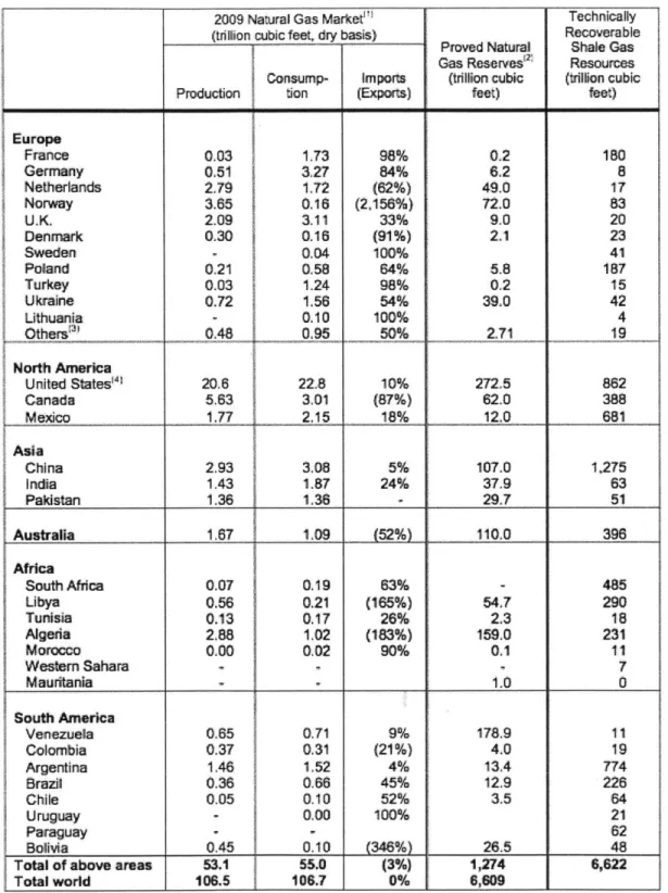
reported in 2011 that an initial estimate of technically recoverable shale gas resources is 6,622 Tcf. The study analyzed 32 countries around the world in addition to the United States. Notable among the results is the fact that China has a technically recoverable
natural gas resource of 1,275 Tcf and Argentina has a natural gas resource of 774 Tcf. The study states that the addition of the identified shale gas resource increases the total world technically recoverable natural gas resources to 22,600 Tcf, an increase of over 40 percent [8]. Table 1-1 below summarizes findings of the study for each country
analyzed. The study did not include Russia or the majority of the Middle East, which are large contributors to the overall world supply of natural gas. The study notes that its total
estimate of shale gas resources is not a global estimate but rather the estimate for the 32 countries analyzed in addition to the United States. For that reason, the global shale gas resource is most likely even higher. Still, estimates like these have a high degree of uncertainty. Shale gas is largely untapped in countries outside the United States despite the enormous resource estimates. The economic, environmental, and societal impacts of
shale gas production in the United States could have important implications for how the resource is exploited worldwide.
2009 Natural Gas Market'I Technically (trillon cubic feet, dry basis) Recoverable
Proved Natural Shale Gas Gas Reserves'2 Resources Consump- Imports (trillon cubic (trillion cubic Production tion (Exports) feet) feet)
Europe France 0.03 1173 98% 02 180 Germany 051 84% 5127 6.8 Netherlands 2,79 1.72 (62%) 49.0 1 Norway 3.65 0.16 (2,156%) 72.0 83 U.K 2.09 3 11 33% 9,0 20 Denmark 0.30 0.16 (91%) 2.1 23 Sweden - 0.04 100% 41 Poland 011| 0.58 64% 5,8 187 Turkey 0.03 1.24 98% 0,2 is Ukraine 0.72 1.56 54% 39.0 42 Lithuania 0.10 100% 4 04ers 095 50% 211 19 North America United States'4 20.6 22.8 10% 272.5 862 Canada 5.63 3.01 (87%) 62.0 388 Mexico 1.77 2.15 18% 12,0 881 Asia China 2.93 3.08 5% 107.0 1,275 India 1.43 1.87 24% 37.9 63 Pakistan 1.36 1.38 29.7 51 Australia 1.87 1,09 52%) 110,0 396 Africa South Africa 0.07 0.19 63% - 485 Libya 0.56 0.21 (165%) 54.7 290 Tunisia 0.13 0.17 26% 2.3 18 Algeria 2,88 1.02 (183%) 159.0 231 Morocco 0.00 0.02 90% 0.1 11 Western Sahara - 7 Mauritania 1.0 0 South America Venezuela 0.65 0.71 9% 178.9 11 Colombia 0.37 0.31 (21%) 4.0 19 Argentina 1.46 1,52 4% 13.4 774 Brazil 0.36 0.66 45% 12.9 226 Chile 0.05 0.10 52% 3.5 64 Uruguay - 0.00 100% 21 Paraguay - j - 62 Bolivia 0.45 j 0.10 (346%) 26.5 48
Total of above areas 53.1
j
55.0 (3%) 1,274 6,622Total world 106.5 106.7 0% O,609
1.5 Historic Natural Gas Economics
Natural gas in the United States did not historically have a smooth path to get to where it is today. The natural gas market was first developed with the help of an interstate natural gas pipeline system that supplied local distribution systems. At this point the market was subjected to cost-of-service regulation by both the Federal
government and state governments, and natural gas production and use grew significantly in this framework during the 1950's, 1960's and into the 1970's. However, after the first oil embargo many energy customers attempted to switch to natural gas. The issue was that price controls and the tightly regulated natural gas market served as disincentives for domestic gas production. This led in part to the perception that U.S. gas resources were limited. From the late 1970's until the late 1980's, legislation essentially outlawed building new gas-fired power plants, lowering the demand for natural gas. However, by the mid 1990's the process of deregulation of wellhead natural gas prices that had begun in the late 1980's was complete and new technology surrounding the natural gas market came to the forefront. Highly efficient and relatively inexpensive combined cycle gas turbines were being deployed, and new upstream technologies were used to developed offshore natural gas resources. The combination of these factors led to a period where domestic gas supplies were perceived to be abundant.
At the turn of the 21 s century, the situation began to change yet again. Concerns arose that domestic natural gas supplies were inadequate. Supplies of natural gas from conventional sources were in decline. Unconventional natural gas resources were too expensive and difficult to produce, and the overall confidence in gas fell sharply. The price of natural gas went through periods of significant volatility. The price volatility in the early 2000's served to accelerate the development of LNG import terminals and
infrastructure, as such projects were deemed economically advantageous. In late 2005, a rapid increase in the price of natural gas finally tipped shale gas into the territory of economically viable. The high natural gas prices at the time were justification for the development, using horizontal drilling and hydraulic fracturing, of the Barnett shale. Shale gas was perceived as a profitable venture, causing many to jump into the industry. As drilling of wells in shale plays increased across the United States at the end of the decade, a glut of natural gas in the market was quick to follow, driving prices down yet
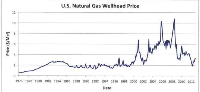
again. The low prices observed led some to question whether shale gas was actually an economically viable option at all. This study hopes to shed some light on the recent economics of natural gas produced from shale formations. Figure 1-7 below shows the historical wellhead price of natural gas in dollars per thousand cubic feet ($/Mcf), helping to illustrate the erratic history of natural gas in the United States.
U.S. Natural Gas Wellhead Price 12 10 ot8 6 0.L 4 V 2 1976 1978 1980 1982 1984 1986 1988 1990 1992 1994 1996 1998 2000 2002 2004 2006 2008 2010 2012 Date
Figure 1-7: Historic U.S. natural gas wellhead price ($/Mcf)
1.6 Implications of Shale Gas Production
Low natural gas prices like those of the past year make it difficult for operators to produce shale gas at a profit. While this puts stress on the operators and may influence some to hold off on future production until prices increase, there are other sectors in the United States that stand to benefit greatly from abundant, cheap natural gas. Two prominent sectors that fit this category are the electric power sector, and the chemical manufacturing sector.
In recent years, electric power generation from natural gas has increased partly due to the low cost of the fuel. However, in addition to the currently low price, natural gas is a desirable fuel for electricity generation for a number of reasons. First, natural gas is the cleanest burning of all fossil fuels because of methane's simple, light structure. In comparison to coal, which is what has been the dominant power generation fuel for
decades, natural gas produces approximately one-half of the CO2 emissions that coal does
per kilowatt-hour. The improvement of natural gas over coal is even more drastic when it comes to other harmful pollutants. Natural gas produces less nitrogen oxides (NOx), sulfur dioxide (SO2), and particulate ash than coal, all by at least one order of magnitude difference [3]. These reduced emissions are critical to any future energy plans that call for the reduction of greenhouse gas emissions, especially in the short term. Another advantage of natural gas over coal is that power plants can be highly efficient. Natural Gas Combined Cycle (NGCC) power plants have efficiencies typically around 50-60%. When high efficiency is combined with low natural gas price, the option becomes economically advantageous. Lastly, natural gas turbines can be ramped up or down quickly to respond to changes in power demand. Even before the low gas prices of late, natural gas was used as a backup source of power that could be quickly brought online when needed. With the projected and environmentally necessary increase in renewable, albeit intermittent, power generation sources, the demand for quick responding backup power will increase. Renewable power sources like solar power and wind have the downfall of unreliability based on unpredictable factors like weather, so using natural gas turbines as a backup to ensure that power supply meets demand will most likely increase in the future. Clearly there are several benefits to natural gas as a fuel for power
generation. Lower-cost natural gas translates into lower-cost power generation, and those savings can be passed on to customers as lower electricity costs.
The chemical manufacturing sector in the United States is inherently tied to the global chemical manufacturing sector. Large companies dominate the sector, and decisions regarding where to locate factories and production facilities are based on the cost of supplies in different locations. Natural gas can be used as both a feedstock and fuel source for many chemical manufacturing processes. For instance, methane is broken down to provide the hydrogen needed to produce ammonia, and natural gas can be the fuel that provides the energy to break down the methane. Ammonia is used as a fertilizer by itself and is also used as a basis for other types of fertilizer for the full range of plants and crops. Similarly, ethane from natural gas can be processed into ethylene, which is the most significant single chemical in terms of volume and value and is the basis for various product categories including plastics, adhesives, soaps, solvents, and paints, to
name a few. The process of transforming ethane into these products also needs a fuel to provide the necessary energy, which natural gas can cleanly do. A
PricewaterhouseCoopers (PwC) study of the impact of shale gas on domestic chemical manufacturing companies found that lower-price natural gas as a result of shale gas production results in big benefits for chemical companies. The study states that the United States could be the lowest-cost producer of ethylene, ahead of Asia and Saudi Arabia Polyethylene, the number one plastic by volume and value, is produced from ethylene that has been converted into long-chain polymers. The PwC study found that the potential selling price of High Density Polyethylene (HDPE) could be reduced by 2.4 times because of the reduction in natural gas costs [9]. Since chemicals are used in an
estimated 90% of all manufactured products, the lower chemical costs that result from lower natural gas prices can bring about lower manufacturing costs which can eventually be passed on to the customers as savings. If natural gas prices remain low, the chemical
sector and its customers all benefit.
2. Current Situation and Challenges 2.1 Supply Increase, Price Decrease
At the current time natural gas production from shale formations is still quite young and developing. Performance data for modem shale gas wells cannot be older
than eight years in the case of wells from 2005. Most wells, especially in younger plays have only been producing natural gas for a few years. Because of the relative novelty of shale gas as a serious portion of domestic supply, the long-term production of these wells remains to be seen. Similarly, longer-term economic, environmental, and societal effects are currently unknown. Despite this, production of natural gas from shale rocks has been and will continue to be extensively studied and analyzed because of its massive potential.
As mentioned above, shale gas production has brought a substantial volume of natural gas to the market, and this trend is likely to increase into the future. The increase in supply has outpaced demand resulting in low natural gas prices, most notably in the past two to three years. While these low prices benefit some, it puts pressure on the operators to keep costs low and production high, which might not always be possible. In fact, as the economic analysis in this study will show, many wells that have been drilled
in the past resulted in a monetary loss for the operating company. With excess supply creating downward pressure on natural gas prices, some smaller operating companies may be forced out of the industry at least until prices rise back to a level that is conducive to profitable wells. For this reason among others, prices may not stay at the low level that they are currently. Yet for the time being the low gas prices pose a formidable challenge to production companies that seek to make a net profit on each of their wells.
2.2 Production Variability
Although low gas prices create an economically challenging situation for
production companies, a larger challenge exists for the entire shale gas industry. As more and more wells are drilled in various plays, it has become apparent that there exists a wide, unpredictable variability in the natural gas production of shale gas wells. Different shale plays have different shale characteristics, so it is quite reasonable to expect
production rates to vary from one play to another, which they do. However, it is also the case that a large variability in production rates exists within the same play. Figure 2-1 shows a histogram of the peak production (in average Mcf/day of the peak month) from all Barnett wells analyzed in this study drilled from 2005 to 2012 [10]. It can be shown that this distribution is lognormal. Table 2-1 summarizes the mean and median peak gas production of the same Barnett wells. Universally, the mean peak production rate is greater than the median peak production rate, which indicates that the distribution is skewed upwards. Also listed in Table 2-1 are the P90 and P10 peak production rates, which are the peak production rates that 90% of wells performed below and 10% of wells performed below, respectively. The spread between the P90 and P10 peak production rates is quite consistent across vintages and is bounded between 4.5 and 5.6. This ratio of approximately a factor of five difference between the top and bottom performing wells solidifies the fact that unpredictable variability can present quite a challenge.
Furthermore, the variability is not spatially dependent at small distance scales. What this means is that while there are "core" areas of plays that on average contain higher
producing wells, within the core or non-core areas there is an equal chance of producing a relatively high volume of gas as there is of producing a relatively low volume of gas.
Most importantly, this variability has not been linked to any characteristics of the land or operating procedures, and is thus totally unpredictable.
900 0
A
E 800 -700 -600 -500 -400 -300 200 II I I I I I 100 0 1000 2000 3000 4000 5000 6Peak Month Gas Production Rate (McflDay)
8000
Figure 2-1: Distribution of peak gas production rate in Mcf/day for all Barnett wells analyzed in this study drilled between 2005 and 2012
1,t51:b 1,5t3 3,421 616 1,689 1,435 3,149 603 5.2 1,794 1,553 3,262 602 5.4 1,767 1,559 3,137 628 5.0 2,005 1,799 3,614 723 5.0 2,225 1,928 3,985 883 4.5 2,383 2,095 4,358 805 5.4 2,056 1,774 3,763 829 4.5
Table 2-1: Summary of peak production rate statistics in Mcf/day for all Barnett wells analyzed in this study drilled between 2005 and 2012
The unpredictable variability of shale gas wells within the same play poses an immense challenge for predicting the economics of shale gas. For one thing, high variability of individual well production translates to difficulty assessing the amount of recoverable natural gas in an area. While on a very large scale the variability could
average out, producers looking to buy or lease acreage to drill are put in the tough position of attempting to assess recoverable resources. Chesapeake Energy recently ran into some problems where, among several issues, they claimed that the value of their land was higher than it actually was. With production rates varying so wildly, it is difficult to accurately assess the value of land. Similarly, production variability adds a large amount of uncertainty to operators' metrics for whether or not a shale gas project is a positive economic investment. That difficulty is exacerbated for small operating companies who might operate one rig at a time and drill ten sites in one year. With a much-reduced ability to absorb financial losses compared to large integrated oil companies, a small operating company is essentially taking a potentially very costly gamble with each well it drills as to whether the project will result in a profit. Though big production companies are taking this same gamble their large amounts of capital allow them to drill enough wells to come close to averaging out the variability, so the gamble is much riskier for small production companies.
Some have claimed that a distinction exists between conventional resource production rationale and shale gas production rationale. In a conventional exploration, development, and production process each prospective well is evaluated on an individual basis. Shale gas development has been referred to as more of a "manufacturing process" where wells are drilled on a statistical basis. Even if this contrast holds true, the
"manufacturing process" of shale gas drilling occurs within an environment of high variability, and a large number of wells would need to be drilled in order for average production to come close to overall mean well productivity. With this production variability in mind, this study performs an economic analysis that essentially illustrates the varying profitability of individual wells within the current environment of high production rate variability.
3. Method for Economic Analysis
This study makes use of a discounted cash flow (DCF) model to calculate a breakeven price of shale gas wells on a full-cycle, individual well basis. Using several inputs, the model calculates the wellhead gas price that generates a 10% internal rate of return (IRR) on an individual well basis for each well analyzed. The model is
programmed as a MATLAB function, which allows flexibility both in the application of the model to distinct well data sets as well as manipulation of resulting data sets for intuitive plots and graphics. The economic model includes the first 20 years of production. Steep production declines and discount rates mean that the majority of revenue for each well comes from the first few years. After breakeven prices are calculated, various types of plots can be created to illustrate and analyze the breakeven prices and associated volumes of shale gas.
There are numerous inputs for the economic model. The revenue stream is mainly defined by each well's initial production data, liquid-to-gas ratio (LGR), and the market price for natural gas liquids (NGLs). The revenue stream also depends on the
decline curve parameters D and n, which will be described in more detail. Costs include the capital expenditures, operating costs, royalty and severance payments, lease costs,
and taxes. The model also makes use of a 1.5% inflation rate. Explanations for the values used for these parameters in the economic model in this study are detailed below.
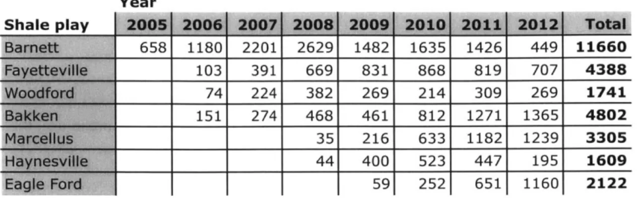
The wells that are analyzed in this study were drilled in the following plays: the Bamett, the Haynesville, the Fayetteville, the Eagle Ford, the Marcellus, the Woodford, and the Bakken. Well characteristic and production data was obtained from the HDPI database for these wells. After exporting the well data, additional filtering was needed to eliminate wells that were either missing data or had data misreported. For instance, wells that had zero gas production, wells that had total depths outside of the possible range for a play, and wells that had negative data values for categories that could only exist as positive values were eliminated from the data set. Also, because full-scale production began at differing times for different shale plays, the first year vintage for each play varies accordingly. All wells in the data sets were drilled horizontally and were active as of March 7, 2013. Table 3-1 below shows the years for which data was included, broken down by each play, as well as the number of wells included from that vintage for each play.
Year 658 1180 2201 2629 1482 1635 1426 449 11660 103731 669 831 868 819 707 4388 74 224 382 269 214 309 269 1741 151 274 468 461 812 1271 1365 48102 35 216 633 1182 1239 3305 44 400 523 447 195 1609 1 591 252 6511 1160 2122
Table 3-1: Number of wells analyzed by play and vintage year
3.1 Revenue Streams in the Economic Model
As mentioned, this study made use of a discounted cash flow model to calculate the wellhead gas price that generates a 10% IRR. The revenue flow in the model is the result of natural gas production and NGL production. In order to calculate the theoretical revenue flow from natural gas, it is necessary to determine an estimated ultimate recovery (EUR) projection for each well.
3.1.1 Decline Curves and EUR
The oil and gas industry has been estimating the ultimate recovery from wells for a long time, as it is important for asset valuation and calculation of proved reserves. However, there is no single way to calculate EUR. One common choice in the industry is to use a reservoir simulation. Unfortunately for shale gas, simulation is not a realistic option because of the lack of understanding of the physics that govern shale gas
production [11], [12]. A second common option for estimating ultimate recovery is the use of a "decline curve," which involves determining a decline trend based on observed production data and projecting that trend forward to reach an EUR. This is the method employed in the economic model used in this study.
Arps carried out the initial work on the decline method [13]. The decline curve that Arps suggested was entirely empirical. Equation 1 below gives the general form of Arps' suggested decline curve.
1 q.(1)
'I (+ bDit)I")
In Equation 1, q is the well's instantaneous production rate, qj is the initial production rate of the well, t is time, and b and Di are constants. The Arps equation is
widely used by analysts to establish shale gas well EURs. Despite its widespread use, the Arps equation is often flawed in a way that leads to an overestimation of EUR [12], [14], [15]. To illustrate the problem, note Figure 3-1 and Table 3-2, which respectively show the normalized production decline trend of the horizontal well vintages in the Barnett shale for 2005, 2007, 2009, and 2011 from [10], and the best-fit b and Di parameters. All of the b parameter values are greater than 1. However, in the limit t -+ oc, with a b value greater than 1, the EUR also goes to infinity which is, logically, a physically impossible value. Some have used the Arps model and assumed a 30 year lifetime of the well, after which production stops [16]. However this method is also incorrect because these wells often remain in transient flow for long periods of time [17],[18], which the Arps equation does not account for. Studies have shown that if the Arps equation is used carelessly with early-life productivity data it can result in an overestimation of EUR by over 100% [14], [19]. 0.9 -0.8 -0.7 -0.6 - 0 .05 vintage 0 '07 vintage 0.5 - 0 '09 vintage. 0 '11 vintage 0.4 - 0 0.3 -0.2 --0 10 20 30 40 50 60 70 80 90 100 Production Month
Table 3-2: Arps decline curve parameters for select Barnett wells
More recently, Ilk et al [14] and Valko [20] have proposed decline curves, which are very similar. The decline curve that is employed in the economic analysis for this study is Valko's rate equation, Equation 2:
q= q,exp (2)
where q is the well's instantaneous production rate, qj is the initial production rate of the well, t is time, and r and n are parameters derived from empirical data. Valko's decline equation accounts for transient flow, and results in finite and reasonable EURs in all situations. This model results in lower EURs than would result if Arps' equation were utilized.
In order to use Valko's "power-law exponential" decline curve, the defining parameters D (used in place of 1/r) and n needed to be determined from empirical data using best-fit curve analysis. Logically, each play has slightly different vintage empirical decline curves because of natural geological variations in the shale formations and their history. Additionally, vintage decline curves from more recent years do not yet have a fully developed shape, and thus resulted in decline curve parameters that cause too aggressive of a decline. For this reason, discretion was used in choosing the decline curve parameters D and n for each play based on averages of the same parameters determined for several of the most historic vintage decline curves for each play.
In the economic model utilized in this study, the power-law exponential decline curve is used with the empirically determined parameters D and n and each individual well's peak gas production rate to create an array of theoretical gas output for each month in a 20 year period. The individual well peak production rate was taken as well data from the HDPI database, and is the amount of gas produced, in Mcf, during the well's highest
producing gas. From there, a theoretical yearly production array was built out to 20 years, assuming that production started in year 0 plus 6 months. Each well's 20-year
production is used in the economic model as one source of revenue flow for that particular well.
3.1.2 Determining the Correct LGR Calculation
The second contribution to a particular well's revenue flow in the economic model comes from natural gas liquids. The amount of NGL associated with each individual well is calculated based on the liquid-to-gas ratio, which itself is a calculated value in barrels of oil equivalent per million cubic feet (boe/MMcf). The well data from the HDPI database includes data on the liquid production of each well in addition to gas production data. Though not completely accurate, the model used in this study assumes that over the 20 year span examined, the production of NGLs declines according to the same decline rate as natural gas production. In reality, liquids production appears to drop off at a faster rate than gas production. Figure 3-2 illustrates this trend through a
cumulative distribution function of the liquid-to-gas ratio of all wells drilled in the Barnett shale in 2006 calculated three different ways. The first method uses the one month peak gas and peak liquids production numbers to calculate the LGR. The second uses the gas and liquids volumes from the first 12 months that a well is on production, and the last uses the cumulative gas and liquids volumes from the entire time that the well has been on production. As can be seen in Figure 3-2, the cumulative distribution
function of LGRs reaches 1 fastest when the cumulative gas and liquid production data is used. This means that the LGRs calculated using cumulative data are in general lower than LGRs calculated using the first twelve month data, which themselves are generally lower than the LGRs calculated using peak gas and peak liquid data. This indicates that the liquid production rate that is present during the peak month declines faster over the cumulative production life of the well than the natural gas production rate. If the gas and liquid production rates declined in equal fashion, the cumulative distribution functions of the LGR's would be identical regardless of which data is used to calculate the LGR.
Cumulaiye Densty Function o( Barne 06 LGR 0.8 -PA G e.1 ...---. U.ULAT.VE LG -PEAK LGR FIRST1 2 LGR 0.1 ... ... ... - CUMULATIVE LGR 0 5 10 15 20 25 30 35 40 45 50 LOR
Figure 3-2: Cumulative Distribution Function of the liquids-to-gas ratio of 2006 vintage Barnett wells calculated using 3 different data sets
Although calculating the LGR using the cumulative gas and liquid production data is perhaps the most accurate, not all wells that were analyzed have the same length of production. For younger wells, the cumulative distribution functions of the LGRs calculated using cumulative production data and the first 12 month production data are rather similar, as there is less of a difference between the data sets used for the
calculations because the length of production is not considerably longer than 12 months. On the other hand as pointed out above, for older wells there is a considerable difference between the LGRs calculated using cumulative data and peak month data. In order to keep consistent and comparable LGRs between vintages, the LGRs that were used in the economic model were calculated using the first 12 month natural gas and liquid
production data.
3.1.3 Natural Gas Liquids Pricing
Natural gas liquids fetch a considerably higher price in the market than natural gas does. This represents a potentially lucrative revenue stream for a natural gas well beyond the revenue of the natural gas itself. Different constituents of natural gas are
priced differently in the market, and like oil and natural gas prices, these prices fluctuate individually. However, the data available for this study does not include the composition of the NGL produced from gas wells, which would be quite complicated. For this reason an approximated, single price for natural gas liquids is established for use in the
economic model. In this study, for each vintage of shale gas wells, the liquids price that is used is 80% of the Cushing, OK WTI Spot Price FOB for the given year. With this price as an input and the derived 20-year liquids production based on the well's LGR and production decline curve parameters, the economic model calculates a portion of revenue flow from natural gas liquids. In total, the gross revenue in the economic model comes from natural gas production and NGL production.
3.2 Costs in the Economic Model
After gross revenue is calculated, royalties and severance payments must come off of the top. One trait of royalties and severance payments is that they come from gross revenue before any other reductions, as a percentage. Another rather simple-to-calculate cost is operating costs. Operating costs are a cost per thousand cubic feet of gas
produced, typically around one dollar or less. In the economic model, the operating cost accrued in a given year is based solely on the amount of gas produced in that year.
The majority of costs involved with shale gas wells come from drilling and completing (hydraulically fracturing) operations. In this economic model, drilling and completing costs were combined as a single capital expenditure value that is assumed to occur in the first year. Several factors such as shale formation depth, geological make-up of layers above the shale, machinery and supply costs, and operating practices due to regulation all affect the drilling and completion costs of a well. Logically because of the differences in the factors mentioned, the different plays analyzed had different capital expenditure values. The economic model was run for each well vintage in all of the plays with capital expenditure applied in two different ways. The first was with a fixed capital expenditure value for each well in a given play that is the same regardless of well date or more importantly well depth (the total length of the well). This is obviously a simplistic view, but little is known or published about drilling and completion costs for wells, especially in the newer plays. The second way in which capital expenditure was applied
in the economic model was using a capital expenditure value for each well that depended on the well depth. A specific per-foot capital expenditure value is calculated for each play by dividing the fixed capital expenditure value by the median total well depth of 2011 vintage wells for each play. When running the economic model using this variable capital expenditure, another input is the total well depth of each well, from which a unique capital expenditure value is calculated for each well. The total depth of the well is the length of pipe from the surface, along the curve and horizontal, to the end of the well, not the vertical depth.
Fortunately for operators, drilling and completion costs as well as lease costs can be written down before taxes according to different schedules. Drilling and completion costs are written down according to United States regulations for both depreciation and intangibles. Lease costs are written down as a percentage cost depletion. This means that each year the percentage of total production that was produced in that year is the
percentage of lease cost that can be written off. In the case of the economic model utilized in this study, these percentages come from the projected production based on the decline curve. An example of a depreciation, intangibles, and depletion schedule for a Barnett shale well is shown below in Table 3-3.
Barnett Shale Tax Write Down Schedule U. 1 14 0.25 0.17 0.13 0.11 0.10 0.10 4 0.1902 4 0.1291 4 0.0960 4 0.0746 4 0.0597 31 0.0488 0.00 0.00 0.0405 0.00 0.00 0.0340 0.00 0.00 0.0288 0.00 0.00 0.0246 0.00 0.00 0.0212 0.00 0.00 0.0184 0.00 0.00 0.0160 0.00 0.00 0.0140 0.00 0.00 0.0123 MM 0.00 0.00 0.0109 NAM 0.00 0.00 0.0097 0.00 0.00 0.0086 0.00 0.00 0.0077