Deformable solids and displacement maps--a multi-scale technique for model recovery and recognition

A Multi-scale Technique

for Model Recovery and Recognition

Stanley Edward Sclaroff

TuFrs UNIVERsITY, 1984

SUBMITTED TO THE MEDIA ARTS AND SCIENCES

SECTION, SCHOOL OF ARCHITECTURE AND PLANNING IN PARTIAL FULFILLMENT OF THE REQUIREMENTS FOR THE DEGREE OF

Master of Science

MASSACHUSETTS INSTITUTE OF TECHNOLOGY June 1991

Massachusetts Institute of Technology 1991 All Rights Reserved

A uthor... Certified by ... Accepted by ... MASSACHUSETTS INSTITUTE OF T19"9"1Y

Ju

U

L

1991

Media Arts and 4 iences Section May 10, 1991

- .- ..--. -. -

.-Alex P. Pentland Associate Professor Computer Information and Design Technology Thesis Supervisor

Stephen Benton Chairperson Departmental Committee on Graduate Studies

Deformable Solids and Displacement Maps:

A Multi-scale Technique

for Model Recovery and Recognition

by

Stanley Edward Sclaroff

Submitted to the Media Arts and Sciences Section, School of Architecture and Planning on May 10, 1991, in partial fulfillment of the

requirements for the degree of Master of Science

Abstract

In this thesis, we formulate a model recovery, recognition, and simulation framework which uses a combination of deformable implicit functions and displacement maps to describe solid objects. Modal deformations, also known as free vibration modes, are used to describe the overall shape of a solid, while displacement maps provide local and fine surface detail by offsetting the surface of the solid along its surface normals. Displacement maps are similar to gray-scale images and can therefore be encoded via standard image compression techniques.

We present an efficient, physically-based solution for recovering these deformable solids from collections of three-dimensional range data, surface normals, surface measurements, and silhouettes, or from two-dimensional contour data. Given a sufficient number of independent measurements, the fitting solution is overconstrained and unique except for rotational symmetries. We then present a physically-based object recognition method that allows simple, closed-form comparisons of recovered models. The performance of these methods is evaluated using both synthetic and real laser rangefinder data and two-dimensional image contours. Finally, we outline how these recovered models can be used efficiently in virtual experiments and simulations - the primary advantage of this approach over the standard polygon-based representations prevalent in computer graphics is that collision detection and dynamic simulation become simple and inexpensive even for complex shapes.

Thesis Supervisor: Alex P. Pentland Title: Associate Professor

Contents

1 Introduction

1.1 Approach . . . . 1.2 O verview . . . . 2 Model Recovery using Deformation Modes

2.1 The Representation . . . . 2.2 Recovering 3-D Part Models From 3-D Sensor Measurements 2.3 Determining Spring Attachment Points . . . . 2.4 Examples of Recovering 3-D Models . . . .

3 Object Recognition

3.1 Using Recovered Mode Values for Recognition . . . . 3.2 Recovering and Recognizing Models . . . . 4 Recovery, Tracking, and Recognition from Contour

4.1 Head Recognition from Contours . . . . 4.2 3-D shape from 2-D contours . . . . 4.3 Dynamic Estimation of Rigid and Non-Rigid Motion...

5 Displacement Maps and Physical Simulation

5.1 The Geometry: Generalized Implicit Functions . . . .

5.2 Computing a Displacement Map . . . . 5.3 Storage and Compression . . . . 6 Conclusion A Programming Shortcuts . . 10 13 . . 15 . . 21 . . 25 . . 30 36 . . . . 37 . . . . 39 59 . . . . 60 . . . . 64 . . . . 66

List of Figures

2-1 Several of the lowest-frequency vibrations modes of a cylinder. . . . . 19

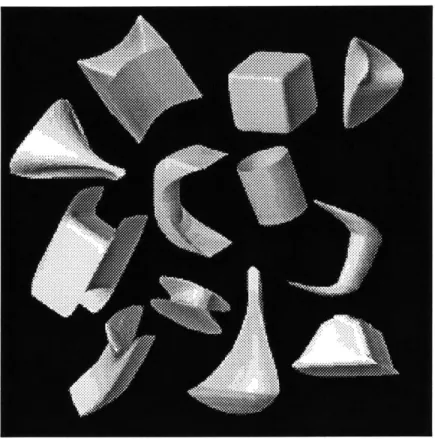
2-2 Some shapes produced by deforming a sphere using 30 modes. . . . . 22

2-3 Using Moment Method for Initial Model Placement . . . . 28

2-4 Fitting geometric objects using sparse 3-D point data . . . . 30

2-5 Fitting laser rangefinder data of a human face. . . . . 32

2-6 Segmenting range data of a human figure into parts . . . . 33

2-7 Incremental fitting to range data of a human figure . . . . 35

3-1 Eight heads used in our recognition experiment . . . . 40

3-2 Recognizing faces from five different points of view. . . . . 41

3-3 How recognition degrades as a function of sensor noise . . . . 43

3-4 Using L2 distance to measure object similarity . . . . 45

3-5 Using normalized dot product to measure object similarity . . . . 46

4-1 Recognizing heads recovered from contours. . . . . 49

4-2 Using a 2-D image contour to recover a 3-D heart model . . . . 50

4-3 Recovering pills from contours and center axes . . . . 52

4-4 A heart's nonrigid motion recovered from contours . . . . 57

5-1 Three frames from a physically-based animation. . . . . 64

5-2 Simulation using a Recovered Head . . . . 68

5-3 Displacement map pyramid. . . . . 69

I gratefully acknowledge the support and advice of my collaborators, Trevor Darrell, Bradley Horowitz, Jun Inagawa, and Sandy Pentland (also my thesis advisor) and the rest of the ThingWorld programming posse: Irfan Essa, Thad Starner, and Martin Friedmann. Special thanks to my thesis readers: Ted Adelson, Frank Ferrie, and Demetri Terzopoulos.

This research was made possible in part by the Rome Air Development Center (RADC) and the Defense Advanced Research Projects Agency (DARPA) under contract No. F30602-89-C-0022. We would like to thank the Harvard Face Archive, Cyberware Labs, and The Visual Computing Group for providing us with range data of human heads.

Chapter 1

Introduction

Recovering higher-level descriptions of images is critical in any machine vision or virtual world scenario. For robots to independently understand, explore, or manipulate their environments, they must be able to extract compact and meaningful representations of the images they gather via a camera. For virtual simulation, we would like to point a camera at a scene and automatically create a computer model - thus gathering the real world, allowing it to coexist with imaginary, computer generated objects. And finally, for image compression to be successful, it will be useful to build up powerful abstractions (i.e., 3-D models) of image data to get the bit rates down to desired levels. The success of each of these depends on how expressive and stable our representation is.

To date, nearly all successful high-level computer vision systems have been unsuccessful at developing a representation which is both general enough and stable enough to be useful in coding a variety of images. Useful computer vision systems have been achieved, but they restrict themselves to a very small variety of shapes - for instance, some parts moving on a factory's conveyor belt - or they assume that they will only encounter certain objects, for which a precise computer model is already known. Such systems solve difficult machine vision problems and are useful within their restricted domains, but they are not useful when it comes to general image coding for high definition video transmission, or when it comes to Al-style image understanding for autonomous creatures who can learn and adapt to new experiences.

There are two contradictory problems which need to be solved before a successful and general machine vision system can be achieved: representation for machine vision, and representation for model recovery and physical simulation. If a computer is to recognize and reason about objects, then it needs a high-level representation which somehow reduces the confounding volume of surface information down to a manageable abstraction. If, however, a computer is to interact with the world, predict behavior, simulate reality, or encode images, then it needs a representation which is general and expressive enough to accurately represent localized surface details and physical behavior. Up until recently, there has been a clear division between representations which provide the necessary abstraction - parametric models - and those which provide the necessary expressiveness - finite element-based, deformable models. Clearly, we would better off with a hybrid method, one that offers the best of both representations.

1.1 Approach

Such a hybrid is not easy to achieve. This is because lurking under all of this is the problem of choosing an appropriate scale. To obtain an abstraction, we reduce shape information down to its fundamental core, but in so doing, we sacrifice local surface detail. A multiscale method is needed, one which allows for choosing the level of detail needed for comparison, simulation, or compression. A standard image compression technique for this is pyramid image encoding. This thesis will explore a similar multiresolution frequency coding method for representing three-dimensional shape. The resulting hybrid representation will be a physically-based, parametric model - based in part on Terzopoulos's work with deformable models and on Pentland's work with modal analysis - and supplemented with a displacement map which will be used to store local surface detail.

The notion of employing physical constraints in shape modeling has been suggested by many authors, however, the seminal paper by Terzopoulos, Witkin, and Kass [47], who obtained 3-D models by fitting simulated rubbery sheets and tubes, has focused attention on

Chapter 1. Introduction

modeling methods that draw on the mathematics used for simulating the dynamics of real

objects. One motivation for using such physically-based representations is that vision is often concerned with estimating changes in position, orientation, and shape, quantities that models such as the finite element method (FEM) accurately describe. Another motivation is that by allowing the user to specify forces that are a function of sensor measurements, the intrinsic dynamic behavior of techniques such as the FEM can be used to solve fitting, interpolation, or correspondence problems.

In this implementation, computer simulated rubber sheets are "shrink-wrapped" over the range data. This rubber sheet is actually a spline, finite element mesh that simulates the reaction of such a sheet to simulated forces - the data points exert forces which essentially attract the sheet. The spline sheets are very good at capturing local detail while staying somewhat stable to noise. And since they are force-based, the resulting deformable models can participate in physical simulations.

Unfortunately, the representation has the drawback that it is not easy to compare two objects. For any mesh-based representation, the only general method for determining if two surfaces are equivalent is to generate a number of sample points at corresponding positions on the two surfaces, and observe the distances between the two sets of sample points. Not only is this a clumsy and costly way to determine if two surfaces are equivalent, but when the two surfaces have very different parameterizations it can also be quite difficult to generate sample points at "corresponding locations" on the two surfaces.

Pentland addressed this problem by adopting an approach based on modal analysis [31]. In this method, the standard FEM computations are simplified by posing the dynamic equations in terms of the equations' eigenvectors. These eigenvectors are known as the object's deformation modes, and together form a frequency-ordered orthonormal basis set for shape. In this representation, objects are described using the force/process metaphor of modeling clay: shape is thought of as the result of pushing, pinching, and pulling on a lump of elastic material. The modal representation, assuming that all modes are employed, decouples the degrees of freedom within the non-rigid dynamic system, but it does not by itself reduce the total

number of degrees of freedom. Thus a complete modal representation suffers from the same non-uniqueness problems as all of the other representations.

The obvious solution to the problem of non-uniqueness is to discard a enough of the high-frequency modes that we can obtain an overconstrained estimate of shape. Use of a reduced-basis modal representation results in a unique representation of shape because the modes (eigenvectors) form a frequency-ordered orthonormal basis set similar to a 3-D Fourier decomposition. Just as with the Fourier decomposition, reducing the number of sample points does not change the low-frequency components, assuming regular subsampling. Similarly, local sampling and measurement noise primarily affect the high-frequency modes rather than the low-frequency modes.

By discarding the higher-order modes, we get a parametric deformable model representation. The parameters are physically meaningful, and correspond to how much bending, tapering, pinching, etc., is needed to represent an object. This is not enough to achieve the goal of a hybrid representation: there is still a trade-off between abstraction and expressiveness, since local shape information (attributed to high frequency modes) is discarded.

To get around this problem, we propose a model recovery framework which incorporates displacement maps to add fine detail to a solid model described by deformable analytic implicit functions. Such maps store surface displacements as a coded relief map, where brighter shades signify positive offsets (peaks), and darker shades signify negative offsets (troughs). Displacement maps are similar to the offsets used for B-splines in that they allow for local and fine-detail control over the shape of the surface. In the context of solid models, displacement maps function by offsetting the analytic surface of the solid along its surface normals. Displacement maps will provide a two-tiered method for describing an object: first the system will compute a low-order modal fit, and then it will do a second pass in which the residual error is stored as a displacement map.

This detail map methodology is especially appealing because the map can be stored like an intensity image. The most useful side-effects of this are that displacement maps can be compressed via standard image compression techniques, and that the representation is

Chapter 1. Introduction 10

especially well-suited for physical simulation. Since the resulting part representation is still an implicit function (displacement maps merely offset the underlying deformed function) intersection and inside/outside measurements are easy to compute.

Thus, as part of this thesis, we will explore some of these aspects of the modal deformation and displacement map combination. In addition, we will outline a method for making a possible "physical connection" between the underlying deformable model and the displacement map.

1.2

Overview

This thesis is built around a core representation: deformable implicit functions supplemented by displacement maps. The purpose will be not only to review and introduce methods for use in model recovery, recognition, and physical simulation, but also to present useful and interesting results of experiments and examples for applications in computer vision and computer graphics. The emphasis (and therefore structure) of the thesis will be split equally between theory and application. Besides this introductory chapter and a short concluding chapter, there are 4 other chapters in this thesis. The chapters are:

Chapter 2: In Chapter 2, we first review the previous work and motivation behind physically-based models in computer vision. In particular, we review the ideas behind modal analysis, what deformation modes look like, and why they are useful in model recovery. As part of this background, the chapter provides a brief review of the Finite Element Method (FEM) and modal analysis. We then present an efficient, physically-based solution for recovering these deformable solids from collections of three-dimensional surface measurements. Given a sufficient number of independent measurements, the fitting solution is overconstrained and unique except for rotational symmetries. The concept of displacement maps is introduced in this chapter, and will be described in more depth in Chapter 5. Examples of model recovery are given using artificial (no noise) range data, laser range data, and integrating data taken from many views of an object.

Chapter 3: The model recovery method described in Chapters 2 produces a vector of mode amplitudes; these are parameters which describe how much of each modal deformation was used in recovering the model. In Chapter 3, we describe a simple, closed-form technique for comparing recovered models. The technique's accuracy, graceful degradation when noise is added to sensor measurements, and plausibility (i.e., If two objects are similar to human observers, are they similar in our recognition system?) are evaluated and discussed using 3-D range-data of human heads, and feature points from geometric objects.

Chapter 4: In Chapter 4, we show how to use the techniques described in Chapters 2 and 3 for recovering, recognizing, and tracking deformable models from two and three-dimensional

contours. By using a variant of weighted least squares, we can enforce volume or symmetry constraints; or by changing weights, we can reflect the certainty of our measurements. We also describe a simple method to include contour normals in model recovery. The examples include head contours taken from range data, and contours taken from an X-ray motion sequence of a human heart beating. In the heart example, we describe a simple recursive filter method which is used to improve the stability of the non-rigid motion recovery.

Chapter 5: This chapter describes our representation and its applications in computer graph-ics terms. Our method can be thought of as generalizing implicit functions by use of polynomial deformations and displacement maps. We then outline a physical simulation technique based on modal dynamics, and include example simulations. Also as part of this chapter, we describe how to compute, store and display displacement-mapped solids. Displacement map interpolation methods are outlined and then demonstrated. Since displacement maps are stored as large floating point image arrays (usually 100x100 or 256x256), there is some concern about the amount of space they occupy in memory or on disk. To get around this problem, we propose using a pyramid-based compression and interpolation scheme which significantly reduces the amount of space needed to store a displacement map.

This thesis presents some work which also appears in journals and conference proceedings. Chapters 2 and 3, were taken in part from [40, 38, 14]. Parts of Chapter 4 appear in an article

Chapter 1. Introduction 12

submitted to the IEEE Workshop on Visual Motion, to be held in Princeton later this year [37]. And finally, parts of Chapters 5 will appear in a SIGGRAPH paper, [41].

Chapter

2

Model Recovery using Deformation

Modes

Vision research has a long tradition of trying to go from collections of low-level measurements to higher-level "part" descriptions such as generalized cylinders [8, 28, 29], deformed superquadrics [33, 34, 42, 10], or geons [7], and then of attempting to perform object recognition. The general idea is to use part-level modeling primitives to bridge the gap between image features (points, edges, or corners) and the symbolic, parts-and-connections descriptions useful for recognition and reasoning [51].

Recently, several researchers have successfully addressed the first of these problems

-that of recovering part descriptions - using deformable models. There have been two classes of such deformable models: those based on parametric solid modeling primitives, such as our own work using superquadrics [33], and those based on mesh-like surface models, such as employed by Terzopoulos, Witkin, and Kass [47]. In the case of parametric modeling, fitting has been performed using the modeling primitive's "inside-outside" function [34, 42, 10, 31], while in the mesh surface models a physical-motivated energy function has been employed [47].

The description of shape by use of orthogonal parameters has the advantage that it can produce a unique, compact description that is well-suited for recognition and database search,

Chapter 2. Model Recovery using Deformation Modes 14 but has the disadvantage that it does not have enough degrees of freedom to account for fine surface details. The deformable mesh approach, in contrast, is very good for describing shape details, but produces descriptions that are neither unique nor compact, and consequently cannot be used for recognition or database search without additional layers of processing. Both of these approaches share the disadvantage that they are relatively slow, requiring dozens of iterations in the case of the parametric formulation, and up to hundreds of iterations in the case of the physically-based mesh formulation.

We have addressed these problems by adopting an approach based on the finite element method (FEM) and solid modeling. This approach provides both the expressiveness and convenience of the physically-based mesh formulation, but in addition can provide much greater accuracy at physical simulation. Thus it is possible to use the models we recover from range data to accurately simulate particular materials and situations for purposes of prediction, visualization, planning, and so forth [39, 31].

More importantly, however, we have been able to obtain develop a formulation whose degrees of freedom are orthogonal, and thus decoupled, by posing the dynamic equations in terms of the FEM equations' eigenvectors. These eigenvectors are known as the object's free

vibration or deformation modes, and together form a frequency-ordered orthonormal basis set analogous to the Fourier transform.

By decoupling the degrees of freedom we achieve substantial advantages:

" The fitting problem has a simple, efficient, closed-form solution.

" The model's intrinsic complexity can be adjusted to match the number of degrees of free-dom in the data measurements, so that the solution can always be made overconstrained.

* When overconstrained, the solution is unique, except for rotational symmetries and degenerate conditions. Thus the solution is well-suited for recognition and database tasks.

The plan of this chapter is to first review our representation. We will then demonstrate its use in obtaining closed-form solutions to the shape recovery problem. This will prepare us for

Chapter 3, where we will demonstrate how closed-form comparison of different object models can be used to obtain accurate object recognition from range data.

2.1 The Representation

Our representation describes objects using the force-and-process metaphor of modeling clay: shape is thought of as the result of pushing, pinching, and pulling on a lump of elastic material such as clay [33, 39, 31]. The mathematical formulation is based on the finite element method (FEM), which is the standard engineering technique for simulating the dynamic behavior of an object.

The notion of employing physical constraints in shape modeling has been suggested by many authors [27, 21, 33]; however, the seminal paper by Terzopoulos, Witkin, and Kass [47], who obtained 3-D models by fitting simulated rubbery sheets and tubes, has focused attention on modeling methods that draw on the mathematics used for simulating the dynamics of real objects. One motivation for using such physically-based representations is that vision is often concerned with estimating changes in position, orientation, and shape, quantities that models such as the FEM accurately describe. Another motivation is that by allowing the user to specify forces that are a function of sensor measurements, the intrinsic dynamic behavior of techniques

such as the FEM can be used to solve fitting, interpolation, or correspondence problems. In the FEM interpolation functions are developed that allow continuous material properties, such as mass and stiffness, to be integrated across the region of interest. Note that this is quite different from the finite difference schemes commonly used in computer vision - as is explained in [23] and [38] - although the resulting equations are quite similar. One major difference between the FEM and the finite difference schemes is that the FEM provides an analytic characterization of the surface between nodes or pixels, whereas finite difference methods do not. All of the results presented in this paper will be applicable to both the finite difference and finite element formulations.

Chapter 2. Model Recovery using Deformation Modes 16 in terms of discrete nodal points. Energy functionals are then formulated in terms of nodal displacements U, and the resulting set of simultaneous equations is iterated to solve for the nodal displacements as a function of impinging loads R:

M + C

+

where U is a 3n x 1 vector of the (Azx, Ay, Az) displacements of the n nodal points relative to the object's center of mass, M, C and K are 3n by 3n matrices describing the mass, damping, and material stiffness between each point within the body, and R is a 3n x 1 vector describing the x, y, and z components of the forces acting on the nodes.

Equation 2.1 is known as the governing equation in the finite element method, and may be interpreted as assigning a certain mass to each nodal point and a certain material stiffness between nodal points, with damping being accounted for by dashpots attached between the nodal points. Inertial and centrifugal effects are accounted for by adding appropriate off-diagonal terms to the mass matrix.

When a constant load is applied to a body it will, over time, come to an equilibrium condition described by

KU=R (2.2)

This equation is known as the equilibrium governing equation. The solution of the equi-librium equation for the nodal displacements U (and thus of the analytic surface interpolation functions) is the most common objective of finite element analyses. In shape modeling, sensor measurements are used to define virtual forces which deform the object to fit the data points. The equilibrium displacements U constitute the recovered shape.

The most obvious drawback of the all physically-based methods are their large computa-tional expense. These methods require roughly 3nmk operations per time step, where 3n is the order of the stiffness matrix and mk is its half bandwidth.1 Normally 3n time steps are required to obtain an equilibrium solution. For a full 3-D model, where typically mk d 3n/2,

the computational cost scales as 0(n3). Because of this poor scaling behavior sometimes equations are discarded in order to obtain sparse banded matrices (for example, in [47] those equations corresponding to internal nodes were discarded). In this case the computational expense is reduced to "only" O(n2_mk).

A related drawback in vision applications is that the number of description parameters is often greater than the number of sensor measurements, necessitating the use of heuristics such as symmetry and smoothness. This also results in non-unique and unstable descriptions, with the consequence that it is normally difficult to determine whether or not two models are equivalent.

Perhaps the most important problem with using physically-based models for vision, however, is that all of the degrees of freedom are coupled together. Thus closed-form solutions are impossible, and solutions to the inverse problems encountered in vision are very difficult.

Thus there is a need for a method which transforms Equation 2.1 into a form which is not only less costly, but also allows closed-form solution. Since the number of operations is proportional to the half bandwidth mk of the stiffness matrix, a reduction in mk will greatly reduce the cost of step-by-step solution. Moreover, if we can actually diagonalize the system of equations, then the degrees of freedom will become uncoupled and we will be able to find closed-form solutions. To accomplish this goal, we utilize a FEM technique known as Modal Analysis; in the remainder of this section we develop this method along the lines of Bathe[23].

To diagonalize the system of equations, a linear transformation of the nodal point displacements U can be used:

U = P (2.3)

where P is a square orthogonal transformation matrix and U is a vector of generalized displacements. Substituting Equation 2.3 into Equation 2.1 and premultiplying by PT yields:

Chapter 2. Model Recovery using Deformation Modes 18 where

M = PTMP;

a

With this transformation of basis set a new system of stiffness, mass and damping matrices can be obtained which has a smaller bandwidth than the original system.

The optimal transformation matrix P is derived from the free vibration modes of the equilibrium equation. Beginning with the governing equation, an eigenvalue problem can be derived

K4; = wiM4; (2.6)

which will determine an optimal transformation basis set.

The eigenvalue problem in Equation 2.6 yields 3n eigensolutions

where all the eigenvectors are M-orthonormalized. Hence

{M

(2.7)

0; i

j

and

0 w _ L3 ... <_ L 2wi (2.8)

The eigenvector

4i

4;

j,

1 <

j

The lowest frequency modes are always the rigid-body modes of translation and rotation. The eigenvector corresponding to axis translation, for instance, has ones for each node's x-axis displacement element, with all other elements being zero. Rotational motion is linearized, so that nodes on the opposite sides of the body have opposite directions of displacement.

Original

Blob-First Order Modes

Shear Taper

Rigid Body Modes

Second Order Modes

Bend Pinch

Figure 2-1: Several of the lowest-frequency vibrations modes of a cylinder.

The next-lowest frequency modes are smooth, whole-body deformations that leave the center of mass and rotation fixed. That is, the (x, y, z) displacements of the nodes are a low-order function of the node's position, and the nodal displacements balance out to zero net translational and rotational motion. Compact bodies (simple solids whose dimensions are within the same order of magnitude) normally have low-order modes that are similar to those shown in Figure 2-1. Bodies with very dissimilar dimensions, or which have holes, etc., can have very complex low-frequency modes.

Chapter 2. Model Recovery using Deformaton Modes 20

eigenvectors 0j, and a diagonal matrix f22, with the eigenvalues wf on its diagonal:

=[41, #2, 03, ... , #3n] (2.9) W2 2 f22 (2.10) 2 W3n

Using Equation 2.10, Equation 2.6 can now be written as:

K4 = M412 (2.11)

and since the eigenvectors are M-orthonormal:

TK4 = f22

(2.12)

From the above formulations it becomes apparent that matrix 4 is the optimal transformation matrix P for systems in which damping effects are negligible.

To also diagonalize the damping matrix C with the same transform, C must be restricted to a special form. The normal assumption is that the damping matrix is constructed by using the Caughey series [23],

P-1 _]k

C = ME ak

[M-K

k=o

Restriction to this form is equivalent to the assumption that damping, which describes the overall energy dissipation during the system response, is proportional to system response. For

p < 2, Equation 2.13 reduces to Rayleigh damping (C = aoM + aiK), and C is diagonalized by 4. Rayleigh damping is the most common type of damping used in finite element analysis

[23].

Under the assumption of Rayleigh damping the general governing equation, given by Equation 2.4, is reduced to

U

Cu

where = aoI + a1 2, or equivalently to 3n independent and individual equations of the form

u0(t) + esi4(t) + Wfi;(t) = i(t) (2.15)

where Z; are modal damping parameters and i;(t) =

TR(t)

In summary, then, it has been shown that the general finite element governing equation is decoupled when using a transformation matrix P whose columns are the free vibration mode shapes of the FEM system [23, 39, 31]. These decoupled equations may then be integrated numerically (see [39]) or solved in closed-form for any future time t by use of a Duhamel

integral (see [31]).

2.2 Recovering 3-D Part Models From 3-D Sensor

Measure-ments

Let us assume that we are given m three-dimensional sensor measurements (in the global coordinate system) that originate from the surface of a single object

X =[z", y, zI, -- -, '" y'", z"]T (2.16)

Following Terzopoulos et al., we then attach virtual springs between these sensor measurement points and particular nodes on our deformable model. This defines an equilibrium equation whose solution U is the desired fit to the sensor data. Consequently, for m nodes with

Chapter 2. Model Recovery using Deformadon Modes 22

Figure 2-2: A sampling of shapes produced by elastically deforming an initial spherical shape using its 30 lowest-frequency deformation modes. As can be seen, a wide range non-rigid motions and their resulting shapes can be described by relatively few deformation modes.

corresponding sensor measurements, we can calculate the virtual loads R exerted on the undeformed object while fitting it to the sensor measurements. For node k these loads are simply

[r3k, r3k+1, r3k+2] = [xyjzj]T - [xk, yk, z] T (2.17)

where

X [X1,yi,zi,--XnYnZn] T (2.18)

are the nodal coordinates of the undeformed object in the object's coordinate frame. When sensor measurements do not correspond exactly with existing nodes, the loads can be distributed to surrounding nodes using the interpolation functions H used to define the finite element model, as described in [23].

Thus to fit a deformable solid to the measured data we solve the following equilibrium equation:

KU=R (2.19)

where the loads R are as above, the material stiffness matrix K is as described above and in

[15], and the equilibrium displacements U are to be solved for. The solution to the fitting

problem is simply

U = K-1R (2.20)

The difficulty in calculating this solution is the large dimensionality of K, so that iterative solution techniques are normally employed.

However a closed-form solution is available simply by converting this equation to the modal coordinate system. This is accomplished by substituting U = 4'U and premultiplying by @T, so that the equilibrium equation becomes

(K - 4JR (2.21)

or equivalently

Chapter 2. Model Recovery using Deformation Modes 24

where R = 4,TR and K = 4,TK@4 is a diagonal matrix (see Equation 2.12). Note that the calculation of 4' needs to be performed only once as a precomputation, and then stored for all future applications. Further, it is normally not desirable to use all of the eigenvectors (as explained in the next section), so that the <D matrix remains of manageable size even when using large numbers of nodes. In our implementation 4, is normally a 30 x 3n matrix, where n is the number of nodes.

The solution to the fitting problem, therefore, is obtained by inverting the diagonal matrix

K:

S= k-In (2.23)

Note, however, that as this formulation is posed in the object's coordinate system the rigid body modes have zero eigenvalues, and must therefore be solved for separately by setting 6; = ri, 1 < i < 6. The complete solution may be written in the original nodal coordinate system, as follows

U = 4(K + J)-14TR (2.24)

where 16 is a matrix whose first six diagonal elements are ones, and remaining elements are zero.2

The major difficulty in calculating this solution occurs when there are fewer degrees of freedom in sensor measurements than in the nodal positions - as is normally the case in computer vision applications. Previous researchers have suggested adopting heuristics such as smoothness and symmetry to obtain a well-behaved solution; however in many cases the observed objects are neither smooth nor symmetric, and so an alternative method is desirable.

We believe that a better, and certainly simpler, method is to discard some of the high-frequency modes, so that the number of degrees of freedom in U is equal to or less than the number of degrees of freedom in the sensor measurements. To accomplish this, one simply row and column reduces k, and column reduces 4, so that their rank is less than or equal to the number of available sensor measurement degrees of freedom. The motivation for this strategy

2_{Inclusion of the matrix L into Equation 2.24 may also be interpreted as adding an external force that}

is that:

* When there are fewer degrees of freedom in the sensor measurements than in the model, the high-frequency modes cannot in any sense be accurate, as there is insufficient data to constrain them. Their value primarily reflects the smoothness heuristic employed.

* While the high-frequency modes will not contain information, they are the dominant factor determining the cost of the solution, as they are both numerous and require the use of very small time steps [39].

* In any case, high-frequency modes typically have very little energy, and even less effect on the overall object shape. This is because (for a given excitatory energy) the displacement amplitude for each mode is inversely proportional to the square of the mode's resonance frequency, and because damping is proportional to a mode's frequency. The consequence of these combined effects is that high-frequency modes generally have very little amplitude. Indeed, in structural analysis of airframes and buildings it is standard practice to discard such high-frequency modes.

Perhaps the most interesting consequence of discarding some of the high-frequency modes, however, is that it allows Equation 2.24 to provide a generically overconstrained estimate of object shape. Note that discarding high-frequency modes is not equivalent to a smoothness assumption, as sharp corners, creases, etc., can still be obtained. What we cannot do with a reduced-basis modal representation is place many creases or spikes close together.

2.3 Determining Spring Attachment Points

Attaching a virtual spring between a data measurement and a deformable object implicitly specifies a correspondence between some of the model's nodes and the sensor measurements. In most situations this correspondence is not given, and so must be determined in parallel with the equilibrium solution. In our experience this attachment problem is the most problematic aspect of the physically-based modeling paradigm. This is not surprising, however, as the

Chapter 2. Model Recovery using Deformation Modes 26 attachment problem is similar to the correspondence problems found in many other vision applications.

Our approach to the spring attachment problem is similar to that adopted by other researchers [42, 47]. Given a segmentation of the data into objects or "blobs," the first step is to define an ellipsoidal coordinate system by examination of the data's moments of inertia. Data points are then projected onto this ellipsoid in order to determine the spring attachment points. We will describe only the simplest form of this method, one that does not adjust for uneven sampling of the data, as the general approach is well known.

2.3.1 Central Moments of Inertia

The center of the object is taken to be its center of gravity, except that because we see only the front-facing surface of the object we must employ a symmetry assumption to determine the z coordinate. After the center of gravity is found, we then determine the object's orientation, which is assumed to be the same as its axes of inertia. The inertia matrix for sample range data consists of the moments of inertia and the cross products of inertia:

f

(y2

- f xydm f (x2 + z2) dm - f yzdm (2.25)

- f xzdm - f yzdm f (x2

+

Since we are integrating over sampled data for the solid, the integrals become summations. In order to make this simplification, we assume that the data points are more or less uniformly sampled, and that each point has the same mass. With this simplification, the matrix becomes:

n n n ZY ±z ) >jxiys i i=1 ia=1i= n n n =

Z

(x

Z)

S

(2.26)

correspond roughly with the axes of inertia for the object. The eigenvector with the smallest eigenvalue corresponds to the most elongated axis of the body, and the eigenvector with the largest eigenvalue corresponds to the shortest axis. Finally, to obtain estimates of the x, y, and z dimensions, we inverse transform the sample points (using the rotation matrix built from the eigenvectors obtained in the previous step), measure the x, y, and z range, and finally double the size estimate along the view direction.

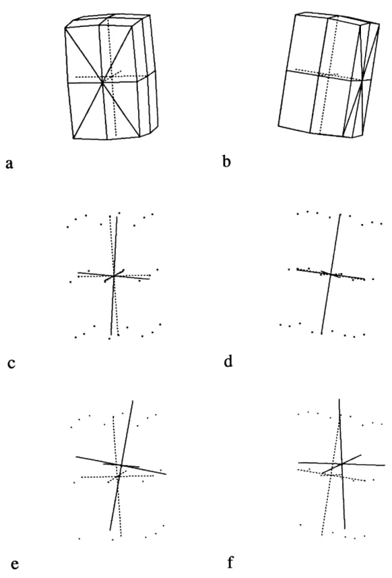
Figure 2-3 shows the results of applying this technique to points sparsely sampled from a box. Notice how the moment method can produce a very good initial estimate of position, orientation and size if sensor data is sampled from all sides of the object, and how - if the data is only take from the front face, or is nonuniformly sampled - partial data can produce an approximation which can vary in accuracy. The top row shows the front view (a) and orthogonal side view (b) of a box and its actual coordinate axes. The middle row (c,d) shows the initial position, size, and orientation calculated via the moment method (shown as solid lines) for a small collection of box surface points. The bottom row (e,f) shows the same orientation information calculated by using only the surface points visible in (a) as input to the moment calculations.

One way to improve the initial estimate would be to push the center of gravity back along the viewing axis. Another is to allow variable point masses when uniform sampling is not available (by uniform sampling we mean uniform sampling in 3-D, uniform sampling in the image plane is not usually uniform sampling 3-D). Generally speaking, the moment method performs well and produces a guess that is correct within ±15 degrees. Therefore, it is sufficient to use what may sometimes be a slightly flawed initial guess as input to spring attachment anyway, and then iteratively refine it (if need be) in tandem with the fitting solution.

2.3.2 Point Projection

This initial estimate of position, orientation, and size defines an elliptical coordinate system. Our attention now turns to attaching springs to the surface of our initial estimate. To establish a correspondence between sensor measurements and the nodes of the undeformed model, each

Chapter 2. Model Recovery using Defomation Modes

Figure 2-3: Using the moment method for initial model placement

--- ...

---sensor measurement, x is translated and rotated into the object's coordinate frame to produce R. The point R is then projected onto the ellipsoid's isoparametric space by use of a normal projection function P(i). This function returns latitude w, and longitude Y.

The projection function P(k) = (r, w) for ellipsoids is computed as follows. We first find

w by observing:

ao- _{=cos7sinL = tan w (2.27)}

aix cos y cos w

where ao, al, and a2 are the x, y, and z axis sizes for the ellipsoid, and (z, #, i)T = k is the

sensor data point in the ellipsoid's coordinate system. From Equation 2.27, we see that:

w = atan( aoy) (2.28)

alx

The remaining parameter, y, is determined by either

S=

atan( or = atan( alzsin) (2.29)

a2x a2y

depending on whether i or 9 is larger.

This projection implicitly defines a correspondence between the sample points and the nodal coordinates. By using the FEM interpolation functions H, the virtual load generated by each data point is then distributed to the nodes whose positions surround the data point's latitude and longitude. We have found, however, that when there are enough nodes, most data points project near a node; consequently, it is sufficiently accurate to distribute these virtual loads to the surrounding nodal points using a simple Gaussian weighting or by bilinear interpolation. This is discussed further in the appendix.

For simple objects (e.g., cubes, bananas, cylinders) our experimental results show that this method of establishing spring attachment points yields accurate, unique object descriptions. It should be noted, however, that because Ik linearizes object rotation it is important that the elliptical coordinate system established by the moment method be sufficiently close to the object's true coordinate system. We have found that as long as our initial estimate of orientation is within +15 degrees, we can still achieve a stable, accurate estimate of shape.

Chapter 2. Model Recovery using Deformation Modes 30

a

ID

Figure 2-4: Front (a) and side (b) views of fitting a rectangular box, cylinder, banana, etc., using sparse 3-D point data with 5% noise. The original models are shown in white, and the recovered models are shown in darker grey. Given the positions of some of the object's visible surface points (as shown in (a)), we can recover the full 3-D model as is shown in the side view

(b).

For complex objects, however, the spring attachment problem is sufficiently nonlinear that we have found that it necessary to establish attachment positions iteratively. We accomplish this by first fitting a solid model as above, and then use that derived model to more accurately determine the spring attachment locations. In our experiments we have found that two or three iterations of this procedure are normally sufficient to produce a good solution to both the spring attachment and the fitting problems.

2.4 Examples of Recovering 3-D Models

2.4.1 A Synthetic Example

Figure 2-4 shows an example using very sparse synthetic range information. White objects are the original shapes that the range data was drawn from, and the grey objects are the recovered

3-D models. For each white object in Figure 2-4(a) the position of visible corners, edges, and face centers was measured, resulting in between 11 and 18 data points. These data points were then corrupted by adding 5 mm of uniformly distributed noise to each data point's x, y, and

z coordinates; the maximum dimension of each object is approximately 100 mm. Note that only the front-facing 3-D points, e.g., those visible in Figure 2-4(a) at the left, were used in this example. Total execution time on a standard Sun 4/330 is approximately 0.1 seconds per model recovery.

Despite the rather large amount of noise and a complete lack of information about the back side of the object, it can be seen that Equation 2.24 does a good job of recovering the entire 3-D model. This is especially apparent in the side view, shown in Figure 2-4(b), where we can see that even the back side of the recovered models (grey) are very similar to the originals (white). This accuracy despite lack of 3600 data reflects the fact that Equation 2.24 provides the shape estimate with the least internal strain energy, so that symmetric and mirror symmetric solutions are preferred.

2.4.2

An Example Using Laser Rangefinder Data

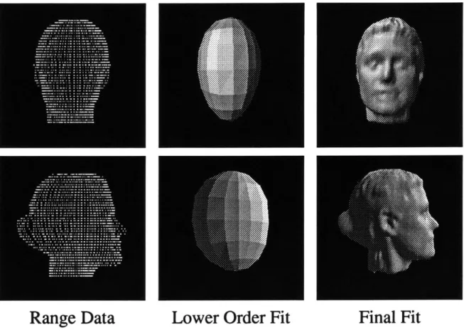
A second example uses 3600 laser rangefinder data of a human head, as shown in the left-hand column of Figure 2-5. There are about 2500 data points. Equation 2.24 was then used to estimate the shape, using only the low-frequency 30 modes. The low-order recovered model is shown in the middle column; because of the large number of data points execution time on a Sun 4/330 was approximately 5 seconds. It can be seen that the low-order modes provide a sort of qualitative description of the overall head shape.

A full-dimensionality recovered model is shown in the right-hand column of 2-5. In the ThingWorld system [39, 35], rather than describing high-frequency surface details using a finite element model with as many degrees of freedom as there are data points, we normally augment a low-order finite element model with a spline description of the surface details. In our representation, this spline description is known as a displacement map. A displacement map can, of course, be similar to splines used by Terzopoulos et al. This provides us with a

Chapter 2. Model Recovery using Deformadon Modes 32

Range Data

Lower Order Fit

Final Fit

Figure 2-5: Fitting laser rangefinder data of a human face. Left column: original range data, Middle column: recovered 3-D model using only low-order modes, Left Column: full recovered model.

a

D

C

d

e

f

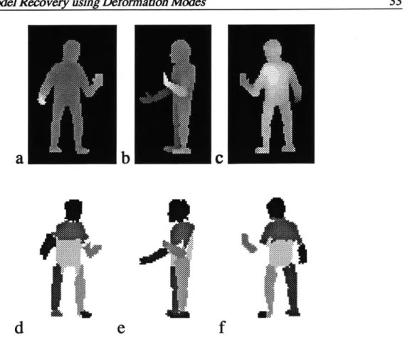
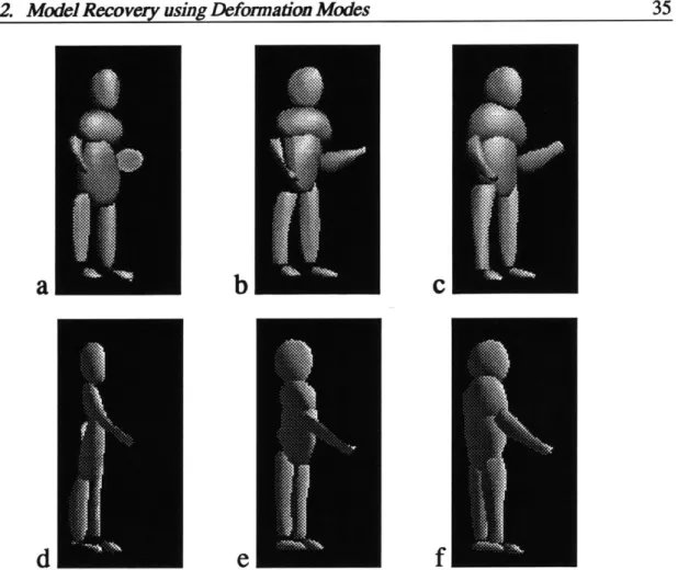
Figure 2-6: Segmenting range data of a human figure into parts. (a,b,c): range data of a human figure from three different viewpoints. (d,e,f): the 2-D segmentations for each view obtained using simple polynomial shape models. Taken from [14].

two-layered representation (low-order finite element model + surface detail spline description

= final model) that we find to be both more efficient to recover and more useful in recognition,

simulation, and visualization tasks than a fully-detailed finite element model. Displacement maps are used to store the residual error between the recovered deformable model and the original data measurements; we will discuss how displacement maps are actually computed in Chapter 5.

2.4.3 An Example of Fusing Multiple Viewpoints

Figure 2-6 shows an example of segmenting laser rangefinger data of a human figure using second order polynomial basis functions, and then integrating the various views into a single

Chapter 2. Model Recovery using Deformation Modes 34

different views. Each image is 128 x 64 pixels in size. For each frame a segmentation was produced using the minimum-description-length algorithm described by Darrell, Sclaroff, and Pentland [14], yielding the segmentations shown in Figure 2-6(d,e,f). Despite use of simple polynomial shape models, a good segmentation was obtained for each view. More importantly, the segmentation is stable across widely different views - despite occlusions - so that data from the same "parts" can be related across the different views. There will be some "smaller" parts of the image (fingers for instance), which, due to the scale of the segmentation, will not be consistent across view. To get around this problem, a size threshold was used [14].

As each of the 2j-D segmentations was produced it was used as input to Equation 2.24, so that a 3-D model of the scene was progressively built up over time. The segmented data was related to the previously-recovered 3-D models by rotating the data using the known changes in camera parameters. The shape of the 3-D model was then re-estimated for all of the available data using Equation 2.24.

Figure 2-7 shows two views of the 3-D models being incrementally fit to the data provided by the 21-D segmentations. It can be seen that as each 21-D segmentation is obtained, it is fused together with the previous segmentations and the 3-D shape model is thus progressively improved. Note that because the 21-D segmentations tend to miss points near the occluding boundaries, the 3-D shapes estimated from a single view (e.g., (a) and (d)) are more flat than they should be.

The final 3-D model, shown in Figure 2-7(c) and (d), encodes the data from all three views in only 276 parameters, yielding an image compression ratio of approximately 300:1 (background pixels excluded) or 900:1 if the three images are considered as independent. The signal-to-noise ratio, a measure of the accuracy of the 3-D description, is 32 dB, so that 99.94% of the data's variance is accounted for by the recovered model.

The dB statistic is computed by comparing the 3-D variance of the original data to the 3-D variance not accounted for by the recovered 3-D models. To compute these variances we measure the 3-D distance between each original data point and the recovered surface along a line from the model's center of mass, and compare this to the 3-D distance between the original

a

D

C

d

e

f

Figure 2-7: Incremental fitting to range data of a human figure. Segmentations from previous figure were used as input to a 3-D shape estimation process. Top and bottom rows show two views of recovered 3-D model. (a,d) shows fit based on points from one 2[-D segmentation, (b,e) fit after two views have been used, (c,f) after all three views. Because the 21-D segmentations are stable, each additional view improves the 3-D model.

data point and the model's center of mass. The segmentation determines which model is used for each point's measurements.

Chapter 3

Object Recognition

Perhaps the major drawback of physically-based models has been that they are not very useful for recognition, comparison, or other database tasks. This is primarily because they normally have more degrees of freedom than there are sensor measurements, so that the recovery process is underconstrained. Therefore, although heuristics such as smoothness or symmetry can be used to obtain a solution, they do not produce a stable, unique solution.

The major problem is that when the model has more degrees of freedom than the data, the model's nodes can slip about on the surface. The result is that there are an infinite number of valid combinations of nodal positions for any particular surface. This difficulty is common to all spline and piecewise polynomial representations, and is known as the knotproblem.

For all such representations, the only general method for determining if two surfaces are equivalent is to generate a number of sample points at corresponding positions on the two surfaces, and observe the distances between the two sets of sample points. Not only is this a clumsy and costly way to determine if two surfaces are equivalent, but when the two surfaces have very different parameterizations it can also be quite difficult to generate sample points at

"corresponding locations" on the two surfaces.

The modal representation, assuming that all modes are employed, decouples the degrees of freedom within the non-rigid dynamic system of Equation 2.1, but it does not by itself reduce the total number of degrees of freedom. Thus a complete modal representation suffers from

the same problems as all of the other representations.

3.1 Using Recovered Mode Values for Recognition

The obvious solution to the problem of non-uniqueness is to discard enough of the high-frequency modes that we can obtain an overconstrained estimate of shape, as was done for the shape recovery problem above. Use of a reduced-basis modal representation results in a unique representation of shape because the modes (eigenvectors) form an orthonormal basis set. Therefore, there is only one way to represent an object, and that is in its canonical position. Further, because the modal representation is frequency-ordered, it has stability properties that are similar to those of a Fourier decomposition. Just as with the Fourier decomposition, an exact subsampling of the data points points does not change the low-frequency modes. Similarly, irregularities in local sampling and measurement noise tend to primarily affect the high-frequency modes, leaving the low-frequency modes relatively unchanged.'

The primary limitation of this uniqueness property stems from the finite element method's linearization of rotation. Because the rotations are linearized, it is impossible to uniquely determine an object's rotation state. Thus object symmetries can lead to multiple descriptions, and errors in measuring object orientation will cause commensurate errors in shape description. Thus by employing a reduced-basis modal representation we can obtain overconstrained shape estimates that are also unique except for rotational symmetries. To compare two objects with known mode values U and 2, one simply compares the two vectors of mode values using a simple distance metric:

Tn

e = ((3.1)

j1

'Note

Chapter 3. Object Recognition 38 or, as we prefer, normalized dot product:

e= ~ ~.2 (3.2)

|IUI||||U211

Vector norms other than the dot product can be employed; in our experience all give roughly the same recognition accuracy. Examples of comparing recovered models using both metrics are show in Figures 3-5 and 3-4 at the end of this chapter.

To recognize a recovered model with estimated mode values U, one compares the recovered mode values to the mode values of all of the p known models:

k - - 12 -., p (3.3)

The known model k with the maximum dot product ek is the model best matching the recovered model, and thus declared to be the model recognized. Note that for each known model k, only the vector of mode values

Uk

The first six entries of 4' are the rigid-body modes (translation and rotation), which are normally irrelevant for object recognition. Similarly, the seventh mode (overall volume) is sometimes irrelevant for object recognition, as many machine vision techniques recover shape only up to an overall scale factor. Thus rather than computing the dot product with all of the

modes U, we typically use only modes number eight and higher, e.g.,

Ek 8 k=l121.., p (3.4)

where m is the total number of modes employed. By use of this formula we obtain translation, rotation, and scale-invariant matching.

The ability to compare the shapes of even complex objects by a simple dot product makes the modal representation well suited to recognition, comparison, and other database tasks. In the following section we will evaluate the reliability of the combined shape recovery/recognition process using both synthetic and laser rangefinder data.

3.2

Recovering and Recognizing Models

There are many ways by which to judge the process of comparing and recognizing 3-D objects. For instance:

" Accuracy: Is it possible to obtain good accuracy from the system?

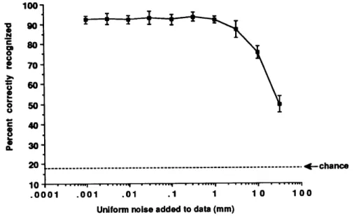
* Graceful Degradation: As noise is added to the sensor measurements, does recognition accuracy degrade slowly?

* Generalization: If two objects are similar to human observers, are they similar to the recognition/comparison system? This is especially useful for database tasks.

In the following sections we will address each of these issues in turn.

3.2.1 Accuracy

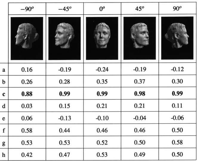
To assess accuracy, we conducted an experiment to recover and recognize face models from range data generated by a laser range finder. In this experiment we obtained laser rangefinder data of eight people's heads from a five different viewing directions: the right side (-90*), halfway between right and front (-450), front (00), halfway between front and left (450), and the left side (900). We have found that people's heads are only approximately symmetric, so that the i450 and t900 degree views of each head have quite different detailed shape. In each case the range data was from the forward-facing, visible surface only.

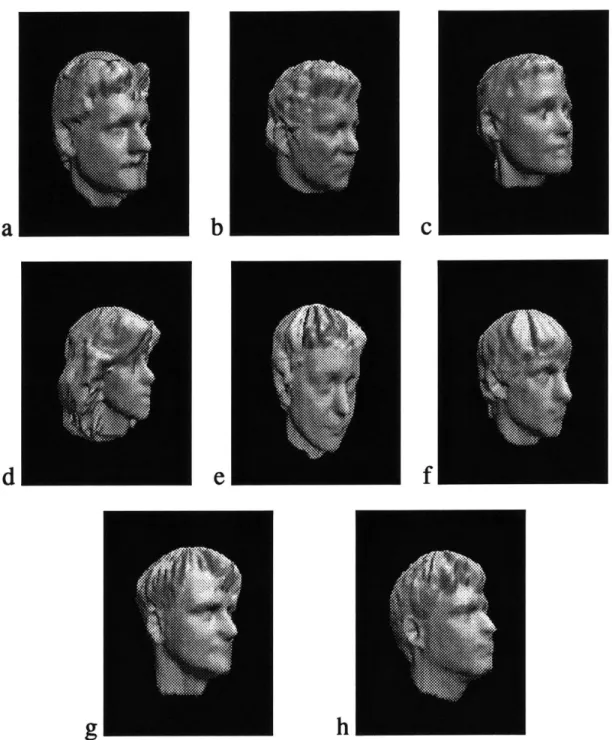
Data from a 3600 scan around each head was then used to form the stored model of each head that was later used for recognition. Full-detail versions of these eight reference models are shown in Figure 3-1; note that in some cases a significant amount of the data is missing. As previously, only the low order 30 deformation modes were used in the shape extraction and recognition procedure. Because the low order modes provide a coarse, qualitative summary of the object shape (see the middle column of Figure 2-5) they can be expected to be the most stable with respect to noise and viewpoint change. Total execution time on a standard Sun 4/330 averaged approximately 5 seconds per fitting and recognition trial.

Chapter 3. Object Recognition 40

a

d

e

f

g

h

Figure 3-1: Eight heads used in our recognition experiment. Note that in some cases there is significant missing data.

-900 -450 00 450 900

a

0.16

-0.19

-0.24

-0.19

-0.12

b

0.26

0.28

0.35

0.37

0.30

c

0.88

0.99

0.99

0.98

0.99

d

0.03

0.15

0.21

0.21

0.11

e

0.06

-0.13

-0.10

-0.04

-0.06

f

0.58

0.44

0.46

0.46

0.50

g

0.53

0.53

0.52

0.50

0.58

h

0.42

0.47

0.53

0.49

0.50

Figure 3-2: Recognizing faces from five different points of view.

Recognition was accomplished by first recovering a 3-D model from the visible-surface range data, and then comparing the recovered mode values to the mode values stored for each of the three known head models using Equation 3.4. The known model producing the largest dot product was declared to be the recognized object. The first seven modes were not employed, so that the recognition process was translation, rotation, and scale invariant.

Figure 3-2 illustrates typical results from this experiment. The top row of Figure 3-2 illustrates the five models recovered from range data from the front, visible surface using

viewpoints of -90*, -45*, 0*, 450, and 90*. Each of these recovered head models look similar,