Decoupling of iron and phosphate in the global ocean

Decoupling of Iron and Phosphate

in the Global Ocean

by

Payal Parekh

B.S., University of Michigan, 1995

Submitted in partial fulfillment of the requirements for the degree of Doctor of Philosophy

at the

MASSACHUSETTS INSTITUTE OF TECHNOLOGY and the

WOODS HOLE OCEANOGRAPHIC INSTITUTION June 2003

@

A u th o r ... ... ... Joint Progr-n in Oceanography/Applied Ocean Science and Engineering

May 2, 2003 C ertified by ... ...-... u ... ... John C. Marshall Professor Thesis Supervisor Certified by. ... Edward A. Boyle Professor Thesis Supervisor Accepted by ... Philip M. Gschwend Chair, Joint Committee for Chemical Oceanography

LINDGREN

INSTITUT

SEFlROM3

Decoupling of Iron and Phosphate

in the Global Ocean

by

Payal Parekh

Submitted to the Joint Program in Oceanography/Applied Ocean Science and Engineering

on May 2, 2003, in partial fulfillment of the requirements for the degree of

Doctor of Philosophy

Abstract

Iron (Fe) is an essential micronutrient for marine phytoplankton often limiting phy-toplankton growth due to its low concentration in the ocean and thus playing a role in modulating the ocean's biological pump. In order to understand controls on global Fe distribution, the decoupling between Fe and P04 and the sensitivity of surface

nutrient concentrations to changes in aeolian iron supply, I use a hierarchy of ocean circulation and biogeochemistry models.

I formulate a mechanistic model of iron cycling which includes scavenging onto sinking particles and complexation with an organic ligand. The iron cycle is coupled to a model of the phosphorus cycle. The aeolian source of iron is prescribed. This system is examined in the context of a highly idealized box model. With appropriate choice of parameter values, the model can be brought into consistency with the relatively sparse ocean observations of iron in the oceans.

I implement this biogeochemical scheme in a coarse resolution ocean general circu-lation model, guided by the box model sensitivity studies. This model is also able to reproduce the broad regional patterns of iron and phosphorus. In particular, the high macro-nutrient concentrations of the Southern Oceans result from iron limitation in the model.

I define a tracer, Fe* that quantifies the degree to which a water mass is iron limited. Surface waters in high nutrient, low chlorophyll regions have negative Fe* values, indicating Fe limitation, because aeolian surface dust flux is not sufficient to compensate for the lack of iron in upwelled waters.

The oceanic residence time of Fe is -285 years in the model, confirming that transport plays an important role in controlling deep water [FeT]. Globally, upwelling accounts for 40% of 'new' iron reaching the euphotic zone.

in the remote Southern Ocean, I study Southern Ocean surface P04 response to

increased aeolian dust flux. My box model results suggest that a global ten fold increase in dust flux can support a P0 4 drawdown of -0.25[LM, while the GCM

results suggest a P0 4 drawdown of 0.5 pM.

Thesis Supervisor: John C. Marshall Title: Professor

Thesis Supervisor: Edward A. Boyle Title: Professor

Acknowledgments

"The ocean is a place of paradoxes." Rachel Carson

My path toward a doctoral degree can hardly be considered direct. There were many dead ends; finding the 'right' question to focus on was an arduous task. At various times I followed roads that led me far astray from my research and during my third year even decided to leave, only to be convinced to continue by John Marshall. At various times, I felt as if I were hitting my head against a wall and the end to the thesis would never be in sight. Then suddenly, the work started coming together and research became easier and fun. That is when I knew my life as an apprentice (aka doctoral student) was coming to an end. Now six years later, after working on two different projects with two different advisors, I am able to reflect on my time as a student. Additionally, as any doctoral student learns, a Ph.D. is due to the collaborative effort of many different people.

Having entered MIT with a background in sedimentary field geology and geo-chemistry, I never envisioned that I would write a modeling thesis. I would like to thank David Glover for developing and teaching the 'Modeling, Data Analysis and Numerical Techniques for Geochemistry' course at WHOI. It has been the best class I took during my graduate career and introduced me to biogeochemical modeling, a field that I did not even know existed prior to taking this course. I appreciate Dave's assistance with research during the early years of my Ph.D. work, his positive attitude and friendly demeanor.

I owe a big thanks to my advisor 'Papa John' Marshall for encouraging me to continue when I wanted to quit. He believed in my abilities when I did not myself. Although my thesis work is far from John's area of expertise, he fully supported my work. In fact, I think John and I have had more political discussions than oceano-graphic discussions! Despite our very different outlooks on the world, we found a way

to respect each other's opinions. I will miss our crazy conversations on the 15th floor of the Green building.

I thank Ed Boyle for offering to be my co-advisor, so I could stay in the chemical oceanography program. Ed has been very patient with all of my questions regarding analytical techniques for measuring iron. He has also made his unpublished data available to me for model comparison.

Working with Mick Follows, my unofficial advisor, has been sheer joy. His unas-suming manner is to be admired. Even when my research was not going well, he always ended our meetings on a positive note, leaving me with a few words of encour-agement. After hashing out ideas on the whiteboard in Mick's office, I always left excited about exploring a new idea.

Jim Moffett and Mike Bacon, my committee members from WHOI, have provided meaningful insights at critical junctures. I appreciate their interest in my work and willingness to travel to MIT for committee meetings.

Although Tina Voelker was not on my committee, she provided me with many helpful comments during the early stages of my thesis. She also shared her insights on being a woman in science and the importance of balancing life and work. I thank her for being such a great mentor and role model.

Some of the most interesting conversations about ocean biogeochemistry occurred in the company of Taka Ito and Stephanie Dutkiewicz. I thank them for their insights, enthusiasm and friendship. I hope to collaborate with them for many years to come. My dear friend, Constantine Giannitsis was a great teacher of numerical methods. He helped me to make sense of finite-difference modeling and various ODE solving schemes. But more importantly, he always made me take a break to smell the roses. I sorely miss the deep conversations I shared with him during lunch on the Green Dot about love, philosophy, politics and life.

Never having written a computer program until my second year at MIT, FOR-TRAN was a menace at times. I had the good fortune of improving my programming

abilities due to Jean Mimi Champin's assistance. I appreciate his endless patience and willingness to help me debug portions of the MITGCM code last summer. In addition to FORTRAN and convincing me that vi is indeed the superior editor, Jean Mimi has also introduced me to the great beers of the world. I will fondly remember the political actions we participated in together, as well as the crazy bicycle rides.

David Ferreira and Martin Losch were kind enough to share with me their ency-clopedic knowledge of Matlab. Despite my endless questions, they continued to hang out with me. Their assistance greatly improved the figures in the thesis. Similarly, Patrick Heimbach has been very helpful whenever I have had problems with LaTeX. I also thank him for giving me his ear when I was depressed or confused about life. He holds a special place in my heart.

I thank Chris Hill and Alistair Adcroft for developing the MITGCM and teaching me how to run my model on parallel computers. Chris always encouraged me when the going was tough. I thank Alistair for his sweet smile, good chocolate and amusing personality.

Bridget Bergquist has been a wonderful classmate. I appreciate her willingness to explain to me the iron measurement papers that I did not understand, and provide useful critiques of my sometimes outlandish ideas about iron cycling in the ocean. I also thank her for her laid back attitude, sweet smile and Midwestern friendliness.

MIT can be a very tough and lonely place. Fortunately, though, the comradery among students in the Green Building is exemplary. I thank my fellow graduate stu-dents for working to improve graduate student life for all stustu-dents in the department and for looking out for one another.

The support staff at WHOI have been extremely helpful with big and small tasks. I thank Joanna Ireland, Julia Westwater, Stacey Brudno Drange, and Marsha Gomes. I thank Rose for caring and always greeting me with a smiling face during those late nights in Clark. Vasco was always offering to give me a ride home during the cold winter nights. I thank him for introducing me to Cape Verdean culture through his

poetry, writings and paintings.

Equally at MIT, there are many people in the Green Building that I owe a big thanks to: Linda Meinke and Charmaine King for assisting me with printing problems; Diana Spiegel for UNIX assistance; Lisa McFarren, Helen Dietrich and Chuck Bowser for helping me navigate through the bureaucratic maze of MIT; Greg Shomo from Techsquare for his general computer assistance, interesting conversations about art and linguistics and his friendship; Bud Brown for help with some of the figures in the thesis, sharing with me his handyman skills and telling me cool hanggliding stories; and Carol Sprague and Vicki McKenna for making sure I got my stipend! I thank Carol also for supporting my activist causes.

Due to my amazing ability to procrastinate, I often ended up working until very late at night to meet a deadline. This provided me the opportunity to form a friend-ship with Tony Palotta-a very special man. I thank him for caring about my well being. I will miss his sweet face and interesting stories.

I am fortunate enough to have made many friends within the department: I thank the lunch and hiking crew for much needed diversions; Susie Carter, Michael Horowitz, and Jess Atkins for the amusing conversations back in the E34 days; Lihini Aluwihare for helping me in the early days at WHOI; Bill Lyons for epic training runs along the Charles River and becoming a friend that I adore; Nili Harnik for her sweet nature; Albert Fischer for being such a good friend when times were tough for me; Fernanda Hoefel for her calmness; Helen Hill and Mary Elliff for being supportive women in the department; the Italian mafia and Patrick Miller down in Woods Hole for their love; Jim Thomson for his positive outlook on life (and being my Woods Hole messenger!); Ariane Verdy for her idealism; and my officemate with the sweet French accent, Fanny

Monteiro for her good nature.

I would like to give a special thanks to Joel Sloman for his daily visits. He has introduced me to the world of art and poetry and often fed me when I was too busy to cook. His ability to remain young and wise at the same time is amazing. I have

learned a lot about love and life from him.

There were numerous people the last few months that took care of me while I was busy writing away: Fernanda, Nico Biassoni, Anke Hildebrandt, Anne 0' Brien, Jen Banister, Jaspal Singh and Hardip Mann, Jen Jacobs and Pedro, Samudra and Lalita Vijay and their son Ghoulam. I thank them for feeding me, giving me a place to stay, and, in general, their friendship. I must also thank Bayard Wenzel for helping me to get a wireless connection at my home and meeting me at new and exotic restaurants around the city.

I would like to give a very big thanks to Oren Weinrib and Alex Rae. They both graciously agreed to help with proofreading and editing the thesis. I thank Alex for always being there for me. Oren must be thanked for many things including introducing me to performance art, sharing with me his Naked Manifesto, engaging me in thought-provoking conversations about politics, love, and life and making sure I always had fun. Both of them have showed me that there is much to learn outside the walls of academia.

Nitin Sawhney and Sunaina Maira have been inspirational activists and academics for me. I admire their ability to combine their quest for social justice and research into one. I will miss the late conversations with Nitin over beer about making academia more responsive to society's needs. I thank Sunaina for always inviting me to really cool political art events around the city.

There were times when MIT has been rough, but there were many communities within MIT and around the Boston area that gave me refuge. I thank my many friends at MIT for giving me the opportunity to get to know you. I fondly remember late night coffee and tea with my architecture buddies, cooking with Ann and Ray for hall feeds in East Campus, all-night costume parties with the Media Lab stars and organizing demonstrations and popular education events with those inclined to fight politically for a more socially just campus.

(AID) to provide support to grassroots organizations in India. I made many friends through AID and I thank them for allowing me to stay involved with my homeland from so many miles away. The fighting spirit of the folks in the Narmada Valley and the survivors of Bhopal are truly inspirational.

Many members of the South Asian Center have been my family away from home. I thank them for taking care of me and allowing me to be in touch with issues immigrants from my corner of the world face in this country. I also thank them for organizing many cultural and artistic events that showcase the diversity of the Indian subcontinent.

I am eternally grateful for meeting the larger global justice community in the Boston area. Working with these wonderful people helped me find a way to stay human and put my radical ideas into action. Organizing demonstrations and teach-ins and taking part in civil disobedience gave me hope that a small group of people can change the world. I count many of you among my closest friends in Boston. Although many of you had no idea what I did at that crazy technical school in Cambridge, you were all very supportive of the radical geek!

I thank my Freedom Rising friends, especially David Solnit for letting me be an honorary member of your affinity group. Building puppets for various demonstrations and hanging out with you in many different cities always made for a nice reprieve from research.

Many friends have introduced me to the arts, from poetry to sculpture to avante-garde performance art to protest art, from Indian classical music to electronic music. I thank you for widening my horizons and giving me a glimpse into how those that use the right side of their brains think.

Last in this list, but first in my heart is my family. Their love and support cannot be expressed in words. I thank my parents, Meena and Prithvish, for just letting me be myself and accepting me as I am. I thank my sweet sister, Aarti, for listening when times were rough. My Foi always checked up on me and has always been so

proud of me. I thank my relatives in India for supporting my academic goals and accepting that my visits back to India were short. I would especially like to thank Ba and Nani for their strength and for passing some of it on to me. I dedicate this thesis to them.

It was a long road and very difficult at times, but now that I have reached the goal, it seemed worth it.

Contents

1 Introduction 23

1.1 Biogeochemistry of Iron in the Oceans . . . . 26

1.2 Prior Modeling Studies . . . . 32

1.3 Increased Aeolian Supply . . . . 34

1.4 Sum m ary . . . . 35

2 Explorations of Biogeochemical Iron Cycling using a Multi-box Model 37 2.1 Global Ocean Biogeochemistry Model . . . . 38

2.1.1 Representation 2.1.2 Iron Cycling .

of Macro-nutrient Cycling . . . . . . 2.2 Model Results . . . .

2.2.1 Case I: Net Scavenging Model . . . . . 2.2.2 Case II: Scavenging-Desorption Model 2.2.3 Case III: Complexation . . . . 2.3 Discussion . . . .

3 Sensitivity of Surface Phosphate to Aeolian welling Strength

3.1 Results: Increased Aeolian Flux Simulations 3.1.1 Increased Dust Flux: Southern Ocean. 3.1.2 Increased Dust Flux: Globally . . . . .

13

Iron Source and

Up-. Up-. Up-. Up-. Up-. Up-. Up-. Up-. Up-. Up-. Up-. Up-. Up-. . . . . . . . .

4 Global Iron Cycling: Simulations Using an Ocean General Circula-tion Model

4.1 Introduction . . . . 4.2 Physical Model...

4.2.1 Residual Circulation . . . . 4.2.2 Temperature and Salinity Sections 4.3 Biogeochemical Component . . . .

4.3.1 Aeolian Flux Forcing Field... 4.3.2 Iron Parameterization . . . . 4.4 Results . . . . 4.4.1 Net Scavenging Results . . . . 4.4.2 Scavenging-Desorption Results . . . 4.4.3 Complexation Results . . . . 4.5 Summ ary . . . .

5 Regional and Global Iron Distributions 5.1 A Tracer of Iron Limitation: Fe*... 5.2 Iron Residence Time . . . . 5.3

5.4 5.5 5.6 5.7

Importance of upwelled iron to the euphotic zone Temporal and Vertical Variations: Comparisons to Sensitivity to Aeolian Forcing . . . .

Sensitivity to Variable Fe:C Uptake Ratio . . . .

Chapter Summary . . . . Data . . . . . . . . . . . . . . . 65 . . . . 66 . . . . 66 . . . . 68 . . . . 69 . . . . 72 . . . . 74 . . . . 76 . . . . 76 . . . . 80 . . . . 80 . . . . 88 89 90 93 94 95 102 108 111 6 GCM simulation: Southern Ocean Phosphate Sensitivity to Increased Aeolian Dust Flux 115 6.1 Aeolian Forcing Field . . . . 116

6.2 Global Distributions . . . . 116

6.2.2 Iron . . . . 6.3 Southern Ocean Results . . . . 6.3.1 Comparison of 'modern' and 'paleo' surface

bution . . . . 6.3.2 Fe* . . . . 6.3.3 Local Source of Iron to the Southern Ocean 6.4 Com m ent . . . .

phosphate

distri-7 Conclusions

7.1 N ext Steps . . . . 7.1.1 Research Recommendations from a Modeling Perspective 7.1.2 On-going Work . . . . 7.2 Final Comments . . . . 118 118 121 123 124 124 125 127 127 128 131

List of Figures

Observed surface P0 4 and chlorophyll a . . . .

Average yearly Fe aeolian flux (mg Fe m 2_yr-1_{, Gao et al.,}

Vertical profile of Fe in the Pacific and the Atlantic . . . . Observed Fe at surface, 1000m and below 2000m . . . . Schematic diagram of iron cycling . . . .

. . . . 24

2001) . . 26

. . . . 28 . . . . 29 . . . . 31

Box model schematic . . . . Sensitivity of deep Fe to scavenging rates . . . . Schematic diagram of scavenging-desorption model . . . . . Sensitivity of deep Fe to scavenging-desorption rate constants Schematic diagram of complexation . . . .

Sensitivity of Fe to scavenging rate and KFe'L . . . .

Sensitivity of L' to scavenging rate and KFeIL . . . . . . .

Sensitivity of Fe to scavenging rate and KFe'L for LT= 4nM

Sensitivity of L' to scavenging rate and KFe'L for LT = 4nM

39 44 46 47 49 51 52 54 55

3-1 Surface S. Ocean P0 4 sensitivity to S. Ocean only dust increase . .

3-2 Surface S. Ocean P0 4 sensitivity to global dust increase . . . .

3-3 Percent Iron in surface Southern Ocean derived from dust . . . . . 3-4 S. Ocean deep Fe response to dust increase and upwelling strength .

4-1 Global residual mean of the model . . . . 4-2 Vertical velocity of model at 50m . . . . 1-1 1-2 1-3 1-4 1-5 2-1 2-2 2-3 2-4 2-5 2-6 2-7 2-8 2-9

4-3 4-4 4-5 4-6 4-7 4-8 4-9 4-10 4-11 4-12 4-13 5-1 5-2 5-3 5-4 5-5 5-6 5-7 5-8 5-9 5-10 5-11 5-12 5-13 5-14 5-15 5-16

Comparison of observed and model temperature . . . . Comparison of observed and model salinity . . . . Aeolian flux field used to force the model . . . .

Observed [P0 4]. ...

Modeled [P0 4] for net scavenging case . . . .

Modeled [FeT] for net scavenging case . . . . Modeled [P0 4] for complexation case . . . .

Modeled [FeT] for the complexation case . . . . Fraction FeL . . . . Modeled surface P04 distribution (Archer and Johnson, 2000)

Modeled FeT distribution (Archer and Johnson, 2000) . . . . .

Zonally averaged section of Fe* in the Atlantic basin . . . . Zonally averaged section of Fe* in the Indo-Pacific basin . . . . Zonally averaged section of Fe* in the Southern Ocean basin... Comparison of modeled and observed Fe profiles at BATS . . . . Comparison of modeled and observed Fe profiles at Station ALOHA Comparison of modeled and observed Fe profiles in the N. Pacific Comparison of modeled and observed Fe profiles in the eq. Pacific Comparison of modeled and observed Fe profiles in the S. Ocean . . . Comparison of modeled and observed surface Fe in the W. Atlantic Monthly modeled surface [FeT] at 100_{N, 45}0_{W . . . .}

Monthly modeled dust flux at 100N, 45W . . . . Comparison of observed and modeled monthly surface [FeT] at Station ALOHA ... ...

Modeled monthly dust flux at Station ALOHA . . . . Seasonal dust deposition (Mahowald et al., 2003) . . . . Modeled [P0 4] response to Mahowald et al. (2003) dust forcing . . .

[Modeled [FeT] response to Mahowald et al. (2003) dust forcing . . .

. . . . 69 70 73 . . . . 75 . . . . 78 79 82 . . . . 83 . . . . 85 . . . 87 88 91 92 92 95 96 97 98 98 100 101 102 103 104 105 107 109

5-17 Variance in intracellular Fe:C ratio (Sunda and Huntsman, 1995) . . . 110

5-18 Modeled [P0 4] response to variable Fe:P ratio . . . . 112

5-19 Modeled [FeT] response to variable Fe:P ratio . . . . 113

6-1 Aeolian flux forcing used for the increased dust flux simulation (Ma-howald et al., 1999) . . . . 117

6-2 Modeled [P0 4] for 'paleo' case . . . . 119

6-3 Modeled [FeT] for 'paleo' case . . . . 120

6-4 Comparison of surface [P0 4] in S. Ocean between 'paleo' and 'modern' case . . . . 122

6-5 Zonally averaged Fe* in the S. Ocean for the 'paleo' case . . . . 123

7-1 Schematic diagram of ecosystem model . . . . 128

List of Tables

2.1 Aeolian Fe dust data . . . .. . . . .. . . .. . .. . . .. 42 2.2 M odel Parameters. . . . . 43

Chapter 1

Introduction

Iron (Fe) is known to be an essential micronutrient for marine phytoplankton capa-ble of limiting phytoplankton growth due to its low concentration (Coale et al., 1996; Martin et al., 1994; Price et al., 1994). Ocean regions with such low Fe concentrations are typically characterized by high surface concentrations of macronutrients, but low chlorophyll (referred to as HNLC regions). The Southern Ocean, northern North Pa-cific and equatorial PaPa-cific are classified as HNLC regions (Figure 1-1). Fertilization experiments have shown primary productivity in these regions responds to Fe addi-tions (Martin et al.,1994; Coale et al., 1996; Boyd et al., 2000). At their outset in the North Atlantic, the deep waters are replete in iron relative to P0 4. However, due to

the different biogeochemistry and decoupling of P0 4 and Fe in the deep ocean, when

the waters upwell again (e.g. in the Southern Ocean and the northern North Pacific), they are depleted in Fe relative to phosphorus. Unless the external aeolian supply is sufficient to offset the deficit, iron is limiting.

Evidence from ice cores (Petit et al., 1999) and sediments (Rea, 1994), in addition to suggestions from numerical models (Mahowald et al., 1999), indicate an increased global aeolian dust supply of 2-5 times during the Last Glacial Maximum (LGM) and an increase as high as 20 times at high latitudes. An increased dust flux might have increased nutrient utilization (Francois et al., 1997; Kumar et al., 1995) and

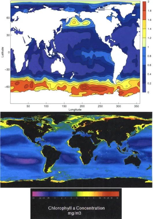
2 1.8 1.6 1.4 30 1.2 0) 1 a) 0 -j 0.8 0.6 -30 0.4 0.2 -60 50 100 150 200 250 300 350 Longitude

Figure 1-1: Top panel displays the surface P0 4 from Conkright et al. (1994) in IM.

The bottom panel displays the yearly averaged chlorophyll a concentration (mg/m 3₎ as sensed by SeaWiFs (Figure courtesy of NASA).

subsequent drawdown of pCO2 in the Southern Ocean during the LGM. However, this hypothesis is yet to be clearly supported. While the field experiments have clearly shown an increase in primary production following iron fertilization in the HNLC regions (Martin et al.,1994; Coale et al., 1996; Boyd et al., 2000) there is, as yet, no clear evidence of a change in export production which would be necessary for modulation of the biological pump of carbon.

While iron may play a significant role in regulating primary productivity and biological drawdown of CO2, the processes controlling its distribution in the global

ocean are poorly understood. Yet, companies have formed (Lam and Chisholm, 2002) with the aim of fertilizing the ocean with iron to mitigate rising CO2 levels in the

atmosphere due to fossil fuel burning.

Much of the emphasis of iron modeling studies have focused on the cycling of Fe within the ecosystem in the upper ocean (Armstrong, 1999; Christian et al., 2002; Leonard et al., 1999; Moore et al., 2002). These models must impose the upwelled iron reaching the euphotic zone. Only two studies have focused on modeling the large scale distribution and maintenance of Fe in the deep waters (Archer and Johnson, 2000; Lef6vre and Watson, 1999), the source for upwelled iron. By building on these previous deep water iron studies, incorporating new understanding and field data, this thesis focuses on understanding what controls the oceanic distribution and supply of iron to the euphotic zone and the effect increased dust flux has on nutrient drawdown in the high latitudes. I test various parameterizations of iron cycling based on its biogeochemical properties within the context of a simple six-box model and a physi-cally more sophisticated three-dimensional coarse resolution ocean general circulation model. I find that the binding of Fe to an organic ligand is able to counteract the loss of Fe due to scavenging. The dominance of scavenging over transport at detph leads to the decoupling between Fe and P0 4 in the deep ocean.

Modern Aeolian Flux (mg Fe/m2/yr) 100 60 10 30-0 1 -30 0.1 -60 -90 0.01 0 50 100 150 200 250 300 350

Figure 1-2: Average yearly Fe flux extrapolated from in situ marine boundary layer measurements by Gao et al.(2001).

1.1

Biogeochemistry of Iron in the Oceans

Like other metals, such as lead and aluminum, iron has an episodic aeolian source to the surface ocean. Global estimates of annual atmospheric iron deposition range between 14-32 x 1012 g Fe (Duce and Tindale, 1991; Tegen and Fung, 1995;

Ma-howald et al., 1999; Gao et al., 2001) with deposition strongest in the North Atlantic and Indian Oceans (Figure 1-2). Dust deposition is lowest in the South Pacific and Southern Ocean.

Assessing the bioavailability and solubility of aeolian-derived Fe is a major research focus. The extent of dissolution in seawater appears to depend on the aerosol source, degree of atmospheric processing, residence time of aerosol Fe in the euphotic zone, particulate load present in surface waters, and the chemical reactions aeolian-derived Fe is subjected to in surface waters (Jickells and Spokes, 2001). Recent studies suggest

the solubility of Fe in dust may be below 5% (Jickells and Spokes, 2001; Spokes and Jickells, 1996).

Other recent evidence indicates that Fe is found in both the soluble (< 0.02 pm) and colloidal size classes (0.02-0.4 pm) (Wu et al., 2001). Previously, due to analytical difficulties, investigators were unable to distinguish between these two forms of Fe. Colloidal iron particles may be less bioavailable than soluble iron (Hudson and Morel, 1990; Wells et al., 1983) and could aggregate into larger particles that sink out of the water column (Honeyman and Santschi, 1989). Since most of the available Fe measurements were not able to distinguish between soluble and colloidal Fe, I do not consider the role of colloids. Rather, in this thesis, 'dissolved' Fe refers to Fe that has passed through a 0.4 pm filter. As we learn more about the nature of Fe-colloids in the ocean, I hope to incorporate this knowledge in the future.

Iron is removed from the water column by scavenging onto sinking particles. Direct quantitative estimates of scavenging rates of Fe have not yet been made, though Bruland et al. (1994) indirectly estimate a residence time for Fe with respect to scavenging between 70-140 years in the water column. Thorium (Th) is a metal that has similar abiological properties to Fe. Bacon and Anderson (1982) calculate an oceanic scavenging rate for Th and also suggest that scavenged Th is released back to the water column. They describe the latter process as a first order reaction proportional to the particulate Th concentration, estimating redissolution rates of 1.33-6.30 yr-1. Since Fe and Th have similar metallic properties, it seems reasonable to speculate that scavenged Fe on particles may also be subject to redissolution.

The vertical profile of iron reflects its role in the biological cycle and atmospheric source. Its vertical profile falls into two categories based on the depth of the mixed layer, rate of biological productivity and dust flux. Regions with deep mixed layers, high productivity and/or weak dust flux are characterized by depleted [FeT] at the surface that increases with depth (Figure 1-3A). In regions with stratified mixed layers, low biological productivity, and strong dust flux, iron builds up near the

0~ * * * 500- * 500- * * 1000- * 1000 -* * 1500- 1500-E * E 2000- * 2000-* * 2500 - x 2500- * * 3000- x - 3000- * 3500 ' ' 3500 ' ' 0 0.2 0.4 0.6 0.8 1 0 0.2 0.4 0.6 0.8 1 [FeT] (nM) [FeT] (nM)

Figure 1-3: Vertical profile in the A) Equatorial Pacific at 3S, 140'W (Johnson et

al., 1997) and B) western North Atlantic at 34.8'N, 57.8'W (Wu et al., 2001).

surface, has a minimum near the base of the mixed layer and then increases with depth (Figure 1-3B). In Figure 1-4A, I present a compilation of surface [FeT] from published and unpublished measurements courtesy of E. Boyle. In high dust flux regions, such as the North Atlantic, surface [FeT] can be elevated. Due to the analytical difficulty of measuring iron, the deep water iron distribution is currently poorly resolved, but it is clear that large scale, deep water Fe gradients do not mirror those of nitrate and phosphate. Rather concentrations, at ~1000m, are highest in the Atlantic ( 0.6-0.8 nM), intermediate in the Indo-Pacific basin (0.4-0.7 nM), and lowest in the Southern Ocean (0.2-0.3 nM) (Figure 1-4B). For depths greater than 2500m, few measurements exist (Figure 1-4C), but suggest highest [FeT] in the Atlantic basin and lower [FeT] in the Southern Ocean and Pacific basin.

Field studies suggest that 99% of dissolved iron (i.e. that which passes through Eq. Pacific (3 S, 140 W) N. Atlantic (34.8 N, 57.8 W)

60P -- & -- - --- J- - - -- --- -6d -- -- - ---- - - --3CP N--- - --- - - --- ---- - - - ---18dW 12d'W 6cP d' 6dE 12E 18W 6d'N - 12-W N---E - 12-18 60%N --- -- - --- ---v i 6 0 'S - - -- - - - - - - - --- - - --- - -

-18d'W 12dW id'W d ~ 6k 12WE 18&W

*< 0.2 + 0.4-0.6

[Fe] (nM)

V0.2-0.4 . > 0.6

Figure 1-4: [Fe] (< 0.4 pam) at the surface (top panel), at 1000-2000m (middle panel) and depths > 2000m (bottom panel). Data sources: Boyle (unpublished); de Baar et

al.,1999; de Jong et al., 1998; Johnson et al., 1997 and references therein; Measures

and Vink, 2001; Nishioka et al.,2001; Obata et al., 1993; Powell and Donat, 2001; Rue and Bruland, 1995; Sedwick et al., 2000; Sohrin et al., 2000; Takeda et al., 1995; Wu and Luther, 1994; Wu et al., 2001

a 0.4 pm filter) is bound to organic ligands throughout the world's oceans (Gledhill and van den Berg, 1994; Rue and Bruland, 1995; van den Berg, 1995; Wu and Luther, 1995; Rue and Bruland, 1997; Gledhill et al., 1998; Nolting et al., 1998; Witter and Luther, 1998; Witter et al., 2000; Boye et al., 2001; Powell and Donat, 2001). The reaction between Fe' and an Fe-binding organic ligand (L'), a molecule with potential binding sites, is:

Fe'+ L' 1 FeL (1.1)

where L' is the Fe-binding organic ligand. The thermodynamic equilibrium can be expressed as:

KFeL = [FeL]/[Fe'] [L'] (1.2)

The source(s), sink(s) and chemical characterization of the ligand is not well known. Estimates of the concentration of ligand range between 0.5-6 nM and most studies suggest only one class of active organic ligand, but two studies (Rue and Bruland, 1997; Nolting et al., 1998) have inferred two ligand classes in the North Pacific and the Pacific sector of the Southern Ocean. Vertical ligand profiles appear nutrient-like with ligand concentration below 1000m remaining relatively constant.

The estimated conditional stability constant of the ligand(s) (KFeL) ranges

be-tween 109.8 M-1 and 1014.3 M without any clear regional pattern. Conditional sta-bility constants are estimated using competitive ligand exchange adsorptive cathodic stripping volt ammetry (CLE-ACSV). A known concentration of a well characterized and purified synthetic ligand is added to a series of field samples containing natu-ral ligands and a range of added metal. Once the synthetic ligand has equilibrated, ACSV is used to measure the concentration of the metal complexed to the added ligand as a function of total metal in solution.

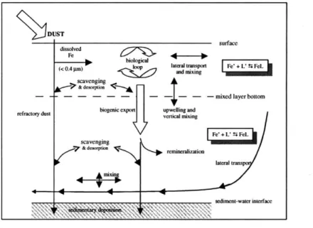
Figure 1-5: Schematic diagram of iron cycling in the global ocean. Figure courtesy of Bridget Bergquist.

Morel, 1978). Since essentially the total Fe pool is complexed, the complexed Fe may actually be bioavailable. Furthermore, extracting iron-binding compounds from sea-water and characterizing certain functional groups within the compound, Macrellis et

al. (2001) found that functional groups known to be present in marine and terrestrial

siderophores are present in the marine environment. This suggests that the ligands are produced biologically by phytoplankton to aid in the uptake of Fe from seawater. The various processes that iron is subjected to, which my model aims to mecha-nistically describe, are summarized in a schematic diagram (Figure 2-1) and will be described in more detail later.

1.2

Prior Modeling Studies

Bruland et al. (1994) and Boyle (1997) suggested that the variable aeolian input into each ocean basin coupled with the biological processes of uptake/regeneration and the metallic property of scavenging could explain the profile of Fe in the world's oceans. Johnson et al. (1997) suggest that iron's complexation to an organic ligand must be controlling the deep water distribution.

Lefevre and Watson (1999) and Archer and Johnson (2000) developed models to examine possible controls on deep water Fe gradients. Lef6vre and Watson (1999) use a ten box representation of the ocean adapted from the PANDORA model (Broecker and Peng, 1986, 1987), parameterizing scavenging of iron onto particles, as well as its biological consumption, remineralization and aeolian deposition. With a scavenging rate of 0.005 yr-1 and solubility of the aeolian iron supply of 2%, their model was able to reproduce the broad features of the deep water iron gradients, although the model yielded higher absolute concentrations in the deep Atlantic (1.6 nM) than observed. Lef6vre and Watson (1999) also introduced a parameterization of complexation and scavenging, which assumed an effective solubility of iron (Fe01) to represent the iron

complexed by a ligand, having a uniform oceanic concentration of 0.6nM. Iron loss was parameterized as a damping toward the effective solubility, -k * ([Fe] - Fesol),

with a timescale of 1/k = 100 years, assuming that only iron which exceeds the effective solubility (i.e. is not bound to the ligand) can be scavenged from the water column. Implicitly, complexation to the ligand is assumed to be very rapid. In this model, deep water concentrations in the Antarctic and the Indo-Pacific were approximately 0.6 nM, and the deep Atlantic is somewhat higher with a concentration of 0.92 nM. The concentrations are higher than currently observed in the Atlantic and Indo-Pacific. However, at the time of that study, this model seemed more consistent with the available evidence, which was interpreted to show that the deep water iron concentration was uniform in all basins. There were fewer measurements and none from the Southern Ocean at that time.

Archer and Johnson (2000), using a three-dimensional global circulation and bio-geochemistry model examined three parameterizations of iron cycling: (A) scavenging only, (B) complexation with one ligand and (C) complexation with two (strong and weak) ligands. In the first case, using a slow scavenging rate (1.6*10-3 yr- 1), the deep water distribution reflects that of a typical nutrient. In the second case, representing complexation with a very strong ligand (K=1.2*101 3_{) of uniform concentration (0.6} nM) results in a uniform deep water Fe distribution, consistent with the observations and their interpretation at the time. In the third case, Archer and Johnson (2000) apply the profile of two iron-binding ligands, a strong ligand (K=1.2*101 3 _M- 1_{) in}

the upper 500 meters with a maximum concentration of 0.5 nM and a weaker ligand (K=3*10" M-1) with concentrations ranging between 1.5-2.5 nM from the surface to depth, as measured by Rue and Bruland (1995) in the North Pacific. This model sim-ulation results in roughly uniform deep water [Fe] in the Atlantic and Pacific basins. In this scenario, excess iron at the surface not utilized biologically was removed from the system,contributed to an unidentified process.

In the light of new data, the first goal of this thesis is to adapt and constrain parameterizations of iron cycling in the deep ocean. I test three parameterizations of iron cycling: (A) net scavenging onto particles, (B) explicit representation of scav-enging and desorption to and from particles, and (C) scavscav-enging and complexation by a single ligand with an imposed total concentration. Here, I test these parame-terizations within the context of a computationally economical, but highly idealized, six-box model and a more sophisticated three-dimensional ocean general circulation model (GCM) to consider which of these parameterizations most successfully captures the observed system as present observations show.

1.3

Increased Aeolian Supply

There is particular interest in the role of iron and aeolian dust supply in the mod-ulation of the surface nutrient concentration of the Southern Ocean and the ocean's biological pumps of carbon (Martin, 1990). Evidence from ice cores (Petit et al., 1999) and suggestions from numerical models (Mahowald et al., 1999) indicates an increased aeolian supply of iron throughout the oceans during periods of glaciation. Numeri-cal ocean models have been used to explore the implications for the carbon cycle by examining the response to imposed surface nutrient drawdown (e.g. Sarmiento and Orr, 1991). Watson et al. (2000) used a simplified ocean biogeochemistry model with explicit representation of iron cycling, forced with glacial-interglacial cycles in South-ern Ocean iron deposition derived from ice core dust records. Their study suggests that a significant fraction of the observed glacial-interglacial change in atmospheric

C02 may be accounted for in this way. Deep water iron cycling is represented in that

model as a particulate scavenging process. In contrast, Lefevre and Watson (1999) found it necessary to increase dust flux globally by a factor of 10 in order to draw-down modeled pCO2 by 50 patm. Archer and Johnson (2000) examined the response of surface phosphate loading to increased aeolian dust supply in their global, three-dimensional model in which deep ocean iron cycling is represented as a combination of complexation to organic ligands and scavenging by particles. The authors suggest that a significant drawdown of the surface macronutrients might be achieved with high ligand concentrations.

The nature of the parameterization of iron, as well as the distribution of and amount of dust flux increase, appears to affect the sensitivity of pCO2 drawdown and surface PO4 drawdown in the Southern Ocean, but varying results are drawn from a diverse suite of models and experiments. The second goal of this thesis is, therefore, to examine these issues through a set of sensitivity experiments in a common framework using the idealized six-box model. Further, I explore the response of surface P04 in the HNLC regions to increased dust flux in the three-dimenensional GCM.

1.4

Summary

It is clear that iron plays an important role in controlling the efficiency of the biological pump and the ultimate drawdown of CO2 by the ocean. Yet, there are many open

questions regarding our understanding of the marine iron cycle and how to represent it in ocean models. This thesis develops an iron biogeochemistry model that draws on previously published models (Archer and Johnson, 2000; Lefdvre and Watson, 1999), but incorporates knowledge from more recent observations and experimental evidence. I incorporate my iron biogeochemical model into a simple multi-dimensional box model and an ocean three-dimensional general circulation model, to test our understanding of controls on deep water iron distribution. Furthermore, I test the effect that increased dust flux has on surface P04 drawdown in the Southern Ocean

to place constraints on the role iron may play in glacial-interglacial cycles.

In Chapter 2, three parameterizations of iron cycling are presented: a net scav-enging case, scavscav-enging-desorption case and complexation-scavscav-enging case. Embed-ded into a simple six-box model, each parameterization is able to reproduce the observed deep water gradients. Results of sensitivity studies to various rate constants and parameterizations are discussed.

The sensitivity of the three iron parameterizations to increased dust flux, as the earth likely experienced during the Last Glacial Maximum (LGM), are presented in

Chapter 3. While each of the parameterizations are able to reproduce, in a broad sense, the modern observed deep water [Fe], their response to increased dust flux varies significantly.

I add the iron biogeochemical parameterizations to an ocean general circulation model in Chapter 4. While all three parameterizations successfully reproduced observed deep water iron gradients in the box model simulations, the ocean general circulation model, with a more sophisticated representation of physics, identifies some differences. Only the complexation case is able to easily capture the observed Fe distribution.

Since the complexation case is the most mechanistic of the three parameterizations and is best able to reproduce modern global iron distributions, I examine the results from this parameterization in greater depth in Chapter 5. I compare modeled profiles to observations and find good agreement, except at the surface in high flux regions such as the North Atlantic. I calculate the global ocean residence time for Fe of ~285 years, indicating that transport must play a key role in controlling Fe distributions. I also find that globally, upwelling accounts for 40% of 'new iron' reaching the euphotic zone. Lastly, I define a tracer, Fe*, that indicates the degree to which a water mass is iron limited.

In Chapter 6, I examine the response of surface PO4 in HNLC regions to

esti-mated LGM dust fluxes (Mahowald et al., 1999) using the ocean general circulation model. While surface PO4 is depleted considerably, there is still excess P0 4 at the

surface, despite a 2.5-fold global increase in dust flux over modern day estimates. I summarize the major findings of the thesis in Chapter 7. Additionally, I recommend areas of further study that would be helpful from a modeling perspective, as well as highlight additional research questions this thesis has brought to light.

Chapter 2

Explorations of Biogeochemical

Iron Cycling using a Multi-box

Model

New data from the Pacific and Southern Oceans (de Baar et al., 1999; Powell and Donat, 2001; Sohrin et al., 2000; Wu et al., 2001; Boyle et al., in prep.) show the distribution of dissolved iron in the deep ocean differs significantly from the uniformity

that previous models, such as those of Lefevre and Watson (1999) and Archer and Johnson (2000) sought to reproduce and understand. Concentrations now appear to be lowest in the Southern Ocean and highest in the Atlantic basin, with a range of values in the Pacific. These models and parameterizations need to be revisited in the light of the new data.

In addition, recent measurements indicate a range in the strength of the condi-tional stability constant and the presence of a significant amount of free ligand. The Lef6vre and Watson (1999) model does not account for these observations. Archer and Johnson's (2000) model adds a weaker ligand in their two ligand scenario, but still has a strong ligand at the surface, which requires the bioavailability of Fe reach-ing the high latitudes to be reduced relative to the rest of the model-domain to keep

surface [P0 4] high in the high latitude surface waters.

Here I aim to build on these previous studies and use more recent data to adapt and constrain the parameterizations of iron cycling in the deep oceans. I will also explore the implications for our understanding of the global nutrient and carbon cycle. In order to allow significant exploration of parameter space, I use a computationally economical, though highly idealized, six-box model of ocean biogeochemistry similar to that of Lefevre and Watson (1999) and Broecker and Peng (1986, 1987). I test three parameterizations of iron cycling with the model: (I) net scavenging onto particles (II) explicit representation of scavenging and desorption to and from particles, and (III) scavenging and complexation. I will show that, provided appropriate parameter values are chosen, each of these parameterizations can reproduce the broad characteristics of the presently observed deep ocean dissolved (< 0.4 pm) iron distribution. However, only the third case concurrently reproduces the observed deep water gradients and the speciation of iron and ligand.

In the following sections I will outline the structure and mechanics of the six-box ocean biogeochemistry model and discuss model results and sensitivities for each of the three iron parameterizations outlined above.

2.1

Global Ocean Biogeochemistry Model

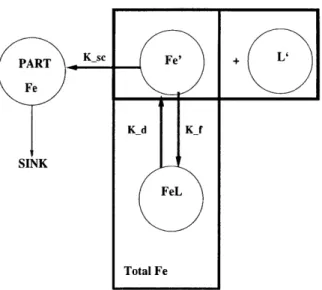
I use a six box model (Figure 2-1) similar in construction to Broecker and Peng's (1986, 1987) Pandora Model, representing the surface and deep waters of the At-lantic, Antarctic, and Indo-Pacific basins. Each basin is divided into two layers, a 100 meter surface layer where biological uptake of nutrients occurs, and a deep layer. Broecker and Peng (1987) tuned volume transports to optimize the modeled 14_C

dis-tribution. I recognize that such highly idealized models have limitations, particularly for quantitative assessments (Broecker et al., 1999; Archer et al., 2000; Follows et al., 2002) but they do provide a useful framework in which to develop clear, qualitative

Figure 2-1: Schematic Diagram of box model adapted from Broecker and Peng (1986, 1987). The arrows represent volume transport (Sv).

understanding and preliminary sensitivity studies of unconstrained rates of various processes.

2.1.1

Representation of Macro-nutrient Cycling

The tracers explicitly carried in my model are phosphate (P0 4), dissolved organic

phosphorus (DOP), total dissolved iron (FeT), and particulate inorganic iron (Fep). Biological uptake and regeneration are indexed to phosphorus. I illustrate the me-chanics of the model's phosphorus cycle with the prognostic equations for phosphate (P0 4) and dissolved organic phosphate (DOP) for the surface and deep Atlantic

(boxes i and ii in Figure 2-1). For the surface:

dP= _{-u - VPO' - F + ADOP}

dt dDOP'

dt -- VDOP + FfDopi - ADOP2

Fe' 4Fe, _{+ Ks} (2.1) (2.2) (2.3) iii V 10 3 6

Surface Atlantic Surface Surface Pacific S. Ocean

20 11 10

H 7 IV 20 1

18 22

5 18

Deep Atlantic Deep Deep Pacific S. Ocean

Superscript numerals indicate the relevant model reservoir. The first term on the right of (1) indicates transport by the model's circulation, the second represents biological export, and the third term the remineralization of DOP. Biological uptake and export are limited by light, phosphate and iron (2.3). In conditions where Fe and light are replete, I assume surface P0 4 to be the limiting nutrient which is exported

with a characteristic timescale, 1/t, of about 1 month. Iron limitation is represented by Michaelis-Menten kinetics. The half saturation constant (K,) is globally uniform but is adjusted, within the range of measured values (Price et al., 1994; Fitzwater

et al., 1996), to optimize the modeled surface [P0 4] and [FeT] distributions. For the

deep:

dPOZ_{dt = -u. VPO" + [l(1}

-fDoPi) + ADOP 2

(2.4)

dDOP"

d -u u= VDOP" - ADOP" (2.5)

In (2.4), the first term on the right represents transport, the second the reminer-alization of sinking particulate matter, and the third the reminerreminer-alization of DOP.

Two-thirds of the exported nutrient (fDOP) enters the surface dissolved organic phosphorus (DOP) pool, while one-third is rapidly exported as particulate P to the deep P04 pool (Yamanaka and Tajika, 1997). The imposed timescale for

remineral-ization of DOP, (1/A), is 6 months.

2.1.2

Iron Cycling

The aeolian source of iron is prescribed, while the loss of iron due to scavenging and iron's role in the biological cycle are modeled explicitly. Total dissolved iron (FeT), and particulate inorganic iron (Fep) are prognostic tracers of the model. The following equations below describe the iron cycle for the surface and deep Atlantic (boxes i and ii in Figure 2-1). The equations for the other basins are similar. For the

surface:

dFe'

T = aFi, - u -VFe - FRFe + ADOP RFe + e (2.6)

dt

dFe 'd = -4e -WskFe' _(2.7)

dt 0z

The first term on the right in (2.6) represents the aeolian source, the second term ocean transport of total iron, the third term biological utilization. Remineralization of DOM is represented by the fourth term on the right multiplied by the Redfield ratio (RFe) between P04 and Fe. The fifth term, JFe represents the interactions

with particles or ligands, which differ between each of the three parameterizations and will be described in more detail below.

Aeolian deposition (Fi,) is the source of iron to the model ocean. Iron deposition data from Gao et al.(2001), Duce and Tindale (1991) and Jickells and Spokes (2001) were used to estimate the source to the surface waters of each basin. Table 2.1 summarizes the various datasets and the values used. The solubility of Fe aerosols (a) in seawater is not well known, although recent studies suggest it may be below 5% (Jickells and Spokes, 2001; Spokes and Jickells, 1996). Based on results of parameter space exploration, we use a = 0.01 for the models discussed here.

Iron is biologically utilized in proportion to P04 with a fixed Fe:C ratio (RFe) and

a C:P Redfield ratio of 16:1. Sunda and Huntsman (1995) have published estimates for the Fe:C ratio that indicate marine phytoplankton decrease their cellular iron re-quirement to optimize growth in Fe-stressed environments, but I have not represented this variability here, as a clear relationship has not been established. The Fe:C ratio is globally adjusted to optimize surface [P0 4] and [FeT].

Evidence from Th isotopes indicates that the mean sinking rate of fine particles is between 500 and 1,000 myr 1 (Cochran et al., 1993). In order to very crudely account for the different sinking rates of large and small particles, we have assumed that 10%

Table 2.1: Aeolian Fe dust data (g Fe yr- 1).

Basin Gao Duce/Tindale Jickells/Spokes Model values

Atlantic 7.73 8.54 6.46 6.46

Southern Ocean 0.071 - - 0.071

Indo-Pacific 5.71 23.5 10.17 10.17

Data sets: Duce and Tindale, 1991; Gao et al., 2001; and Jickells and Spokes, 2001.

of particles are large with a sinking rate of 20,000 myr- 1 and 90% are small particles with a sinking rate of 1,000 myr-1, yielding an average sinking rate (W.) of 2,900 myr-1.

The deep equations for iron are:

dFe" _{= -u VFei +}

FRFe(1 - fDOP)+ ADOP"RFe

dt T _(2.8)

+ Jeii

dFe" F

d = -Jie - Ws Fep (2.9)

I examine three different parameterizations for the geochemical processes: (I) net scavenging (II) scavenging and desorption, and (III) scavenging and complexation. In case I and II, I do not differentiate between complexed and free iron and assume that the total iron pool is subjected to all geochemical processes. In case III, I explicitly model complexation and differentiate between free iron and complexed iron.

2.2

Model Results

While I will focus on the iron distribution in this discussion, the phosphate distri-bution, which is explicitly controlled by iron limitation here, also provides a consis-tency check on the model. For solutions in which iron distribution is reasonable, the phosphate distributions are in good agreement with observations. Surface [P0 4] is

Definition Fe:P ratio fraction of DOP Depth of surface Depth of deep b Aeolian Depositi Fe dust solubilit Biological uptak Remineralization Scavenging rate Backscavenging Particle sinking Iron half saturat Ligand conditior

Table 2.2: Model Parameters Value

adjustable parameter 0.67

box loom

ox 3900m

on rate see Table 1

y1% e rate 1 month-rate 0.5 yr-i variable rate variable velocity 2,900 myr-1

ion constant adjustable parameter al stability constant variable

elevated in the Southern Ocean box, depleted in the Atlantic box and intermediate in the Indo-Pacific box. Deep [P0 4] increases from the Atlantic to the Indo-Pacific.

2.2.1

Case I: Net Scavenging Model

Boyle (1997) suggested that the deep water distribution of iron may be modeled using simple parameterizations of aeolian deposition, biological uptake and remineralization of organic matter, and a representation of net scavenging to particles. Such a model is highly idealized, and does not attempt to explicitly represent the details of the biogeochemical processes, but it could be the simplest viable prognostic model for iron in the ocean. It has only one adjustable parameter and does not attempt to describe poorly understood details of the biogeochemical processes.

Here, I examine whether this parameterization can reproduce the broad basin to basin and surface to deep ocean observed gradients of dissolved iron. In this formula-tion FeT is scavenged and utilized biologically. This parameterizaformula-tion is conceptually similar to the no-ligand model of Lefevre and Watson (1999). I impose the regional variations in aeolian supply and examine the sensitivity of the dissolved iron distri-bution to the net scavenging rate. In this case the loss of iron is modeled simply

Symbol RFe fDOP h H a /t A k₈c kb WS Ks KFeL

2.5

deep Atlantic

deep Southern Ocean deep Indo-Pacific

2-1 -

-0 - i

1 2 3 4 53 6 7

scavenging rate (knetsc 10- yr-)

Figure 2-2: Sensitivity of deep [FeT] to scavenging rates. For slow scavenging rates,

(knetsc <.001), the FeT distribution is nutrient-like. For intermediate scavenging rates,

.004< knetsc <.006, the observed gradients are reproduced. For knetsc>.006, the sense of gradient is reproduced, although mean concentrations are lower than observed.

as a first-order scavenging process, limited by the dissolved free Fe concentration. Scavenged iron is transfered to the particulate pool, Fe,, with rate constant -knetsc,

and is stripped from the water column as the particles sink. For the net scavenging (and scavenging-desorption) case Fe:C is 25 pmol:1 mol. Here, then

JFe = knetscFeT. (2.10)

Figure 2-2 shows the deep ocean, dissolved iron concentrations in each of the three modeled regions (Atlantic basin, Southern Ocean, Pacific basin) as a function of the net scavenging rate. Each cluster of three bars represents the solution of the model at a particular value of scavenging rate. The relative lengths of the three bars

reflect the basin to basin gradients of deep iron in each solution. In the case of a slow net-scavenging rate (knetse = 0.001 yr 1), the deep water distribution is that of a typical nutrient with the deep Indo-Pacific iron concentration greater than the deep Southern Ocean which is greater than the deep Atlantic. The result is unsurprising, but the gradients are not as observed. For stronger scavenging, knetsc >.004 yr-, the observed deep water Fe gradients (Atl>Indo-Pacific>Southern Ocean) are repro-duced. However, when knetsc >.006 yr-1, though the inter-basin gradients remain of the correct sign, the mean ocean deep water [FeT] becomes much too low.

This simple model, representing the basin variations of the aeolian supply and a uniform, net scavenging rate can reproduce the unique deep water iron signature provided that 0.004 yr-l< k8e < 0.006 yr-1. This is consistent with the previous

study of Lefevre and Watson (1999).

2.2.2

Case II: Scavenging-Desorption Model

While the highly simplified model of Case I can reproduce the broad, basin-to-basin gradients of the dissolved iron distribution, it does not resolve the biogeochemical processes at work. In Cases II and III, I introduce more detailed parameterizations which attempt to represent processes known to be, or likely to be, at work in the ocean. I ask if these more detailed models can reproduce the observations and, if so, what constraints can be placed on system parameters by the observations?

Thorium is produced in the ocean by radio-decay and is subsequently scavenged out of the water column by sinking particles. Bacon and Anderson (1982), using oceanic observations of thorium isotopes, have estimated a scavenging rate between 0.2-1.28 yr-1. This is much faster than the net scavenging rate for iron implied in our model (case I), but does not represent the net scavenging rate for Th. Bacon and Anderson (1982) suggest that scavenged Th is also desorbed from particles, i.e. released back to the water column, and also infer from data a rate at which this occurs. Since Fe and Th have similar metallic properties, I consider it likely that iron