Statistics of lowest droplets in two-dimensional Gaussian Ising spin glasses

HAL Id: hal-00000029

https://hal.archives-ouvertes.fr/hal-00000029

Submitted on 25 Oct 2002

HAL is a multi-disciplinary open access

archive for the deposit and dissemination of

sci-entific research documents, whether they are

pub-lished or not. The documents may come from

teaching and research institutions in France or

L’archive ouverte pluridisciplinaire HAL, est

destinée au dépôt et à la diffusion de documents

scientifiques de niveau recherche, publiés ou non,

émanant des établissements d’enseignement et de

recherche français ou étrangers, des laboratoires

Statistics of lowest droplets in two-dimensional Gaussian

Ising spin glasses

Marco Picco, Felix Ritort, Marta Sales

To cite this version:

Marco Picco, Felix Ritort, Marta Sales. Statistics of lowest droplets in two-dimensional Gaussian Ising

spin glasses. Physical Review B: Condensed Matter and Materials Physics (1998-2015), American

Physical Society, 2003, 67, pp.184421. �10.1103/PhysRevB.67.184421�. �hal-00000029�

ccsd-00000029 : 25 Oct 2002

Statistics of lowest droplets in two-dimensional Gaussian Ising spin glasses

M. Picco(1)_{, F. Ritort}(1,2)_{and M. Sales}(2)

(1) LPTHE, Universit´e Pierre et Marie Curie, Paris VI et Universit´e Denis Diderot, Paris VII Boite 126, Tour 16, 1er _{´etage, 4 place Jussieu, F-75252 Paris Cedex 05, France}

(2) Departament de F´ısica Fonamental, Facultat de F´ısica, Universitat de Barcelona Diagonal 647, 08028 Barcelona,Spain

A new approach to determine the value of the zero-temperature thermal exponent θ in spin glasses is presented. It consists in describing the energy level spectrum in spin glasses only in terms of the properties of the lowest energy droplets and the lowest droplet exponents (LDEs) λl, θl

that describe the statistics of their sizes and gaps. We show how these LDEs yield the standard thermal exponent of droplet theory θ through the relation, θ = θl+ dλl. The present approach

provides a new way to measure the thermal exponent θ without any assumption about the correct procedure to generate typical low-lying excitations as is commonly done in many perturbation methods including domain wall calculations. To illustrate the usefulness of the method we present a detailed investigation of the properties of the lowest energy droplets in two-dimensional Gaussian Ising spin glasses. By independent measurements of both LDEs and an aspect-ratio analysis, we find θ(2d) ' −0.46(1) < θDW(2d) ' −0.287 where θDWis the thermal exponent obtained in domain-wall

theory. We also discuss the origin of finite-volume corrections in the behavior of the LDE θl and

relate them to the finite-volume corrections in the statistics of extreme values. Finally, we analyze some geometrical properties of the lowest energy droplets finding results in agreement with those recently reported by Kawashima and Aoki20_{. All in all, we show that typical large-scale droplets are}

not probed by most of the present perturbation methods as they probably do not have a compact structure as has been recently suggested. We speculate that a multi-fractal scenario could be at the roots of the reported discrepancies on the value of the thermal exponent θ in the two-dimensional Gaussian Ising spin glass.

I. INTRODUCTION.

Despite three decades of work in the field of spin glasses major issues related to their low-temperature behavior still

remain unresolved1_{. Although important achievements have been obtained in the understanding of mean-field theory}2

the appropriate treatment beyond mean-field to include short-range interactions is yet to be found. The absence of a successful analytical approach to deal with this problem corroborates the present state of our knowledge, often misguided by a non-accurate, if not confusing, interpretation of the numerical data. This situation has generated a hot debate about the correct physical interpretation of the available numerical data. Leaving aside the long-standing

controversy whether replica symmetry breaking is or not a good description of the spin-glass phase3_{, there are still}

unresolved issues which are not as striking but evidence our ignorance about some fundamental questions.

One among these problems is the correct value of the thermal exponent in two-dimensional (2d) Gaussian Ising spin glasses (GISG). This question has received attention from time to time during the last two decades but not enough to settle it definitively and explain the origin of some of the reported discrepancies. The study of the low-T properties of

the 2d GISG starts with the work by McMillan who proposed4_{that thermal properties in spin glasses are determined}

by the scaling behavior of the typical largest excitations (commonly referred as droplets) present in the system. This idea has been further elaborated and extended to deal with equilibrium and dynamical properties of spin glasses in

a scenario nowadays referred to as droplet model6_{. The low-T behavior in spin glasses is determined by a spectrum}

of large scale gapless droplets with typical length L and energy cost E ∼ Lθ_{, θ being the thermal exponent. As}

these droplets correspond to flipping some domains of spins (assumed to be compact clusters), the energy cost of these excitations arises from the set of unsatisfied bonds on their surface. The striking low-T behavior in spin glasses arises from multiple energy cancellations occurring at the surface of the droplet. These cancellations can be seen as the result of a competition between energy and entropy effects: as the droplet becomes progressively larger there are more available conformations for the surface to minimize the energy cost of the unsatisfied bonds. In the absence of cancellations one would expect θ = (d − 1)/2. However, as these cancellations are very important, the inequality θ < (d − 1)/2 holds and θ is by far less than the maximum value (d − 1)/2. The value of the thermal exponent

θ characterizes the low-T critical behavior as it is related to the correlation length exponent ν where ξ ∼ T−ν _by

the identity ν = −1/θ. McMillan also used domain-wall renormalization group ideas to introduce a practical way

to determine the leading energy cost of these low-lying large-scale excitations5_{. The method consists in measuring}

the energy defect of a domain-wall spanning the whole system obtained by computing the change of the ground state energy when switching from periodic to anti periodic boundary conditions in one direction. Several works have

used McMillan’s method to determine the value of θ in two and three dimensions7,8_{. Hereafter, in order to keep}

the discussion as clear as possible, we will denote by θDW the estimate of the exponent θ obtained by domain-wall

calculations. The initial value for θDW reported by McMillan is θDW = −0.281(5) for pretty modest lattice sizes

L = 3 − 8. Recent numerical results with much more powerful algorithms have reached sizes L ' 500 and confirmed

the initial result with much larger accuracy22,24,27 _θ

DW = −0.287(4). These studies would definitively close the

problem if it were not by the existence of other alternative estimates of the exponent θ, largely consistent among

them, which yield a quite different value θ ' −0.47(2). We will denote this estimate by θT F as several of these

methods use transfer matrix18_{. However, a word of caution is necessary here as the Monte Carlo method and other}

approaches that are not based on transfer matrix methods report values compatible with that estimate. For instance,

Kawashima and Aoki used another method to estimate the stiffness exponent20_{. The idea is to generate a droplet}

inside a box of size L × L that includes a fixed central spin, with the following procedure. First, the ground state is found with a standard algorithms (we will denote it by the reference configuration). Afterwards, the spins at the boundaries of the box are fixed and the central spin is forced to flip respect to the reference configuration. The droplet of minimum energy that includes the central reversed spin and does not touch the boundaries is computed. The spanning length of the droplets generated in this way allows to define the fractal dimension of both the surface (or perimeter for the two dimensional case) and the volume. It is found that these minimum energy droplets have a fractal volume dimension smaller than 2 and the thermal exponent is θ = −0.42(5) in agreement with results obtained

from MC methods26 _{and heuristic optimization algorithms}19_{. A similar study of minimum energy clusters in the}

three-dimensional Edwards-Anderson model also reports evidence that θDW is an upper bound to the actual value of

the thermal exponent21.

The accuracy of previous estimates is poorer than the values obtained through the domain-wall method as they deal, in one way or another, with all possible excitations and not only with the calculation of ground state energies. More recently, another method has been used to estimate the value of θ. It consists in perturbing the original Hamiltonian

H0 with a term ²P, where P stands for the perturbation and ² for its intensity. For example, P can be the overlap

between the actual configuration and the ground state of the original Hamiltonian H0. As ² varies the new ground

state of the total Hamiltonian H = H0+ ²P remains unchanged until a certain value ² = ²cis reached where a excited

energy level of H0 becomes the new ground state of H. The overlap between the old and the new ground states as

well as the value of the shifting energy provoked by the perturbation links its energy cost E with its size providing

another way to estimate θ. We will denote by θP the estimate obtained in this way. This method has been recently

used in the 2d GISG by Hartmann and Young23 _{reporting the following value θ}

P ≈ −0.31. Although slightly more

negative than θDW, both θDW, θP appear to be statistically compatible. Yet more accurate estimates are needed to

confirm whether θP = θDW.

This last method and the domain-wall method have in common the same feature, i.e. they perturb the original Hamiltonian in one way or another to probe the characteristic energy of excitations that are supposed to be the

typical ones that determine the low-T thermodynamic properties. In fact, the estimate θDW can be considered as a

particular example of θP, where the perturbation consists in reversing all the bonds in one of the surfaces of the box.

This raises the important question whether the different estimates of θP, obtained by considering different class of

perturbations, are different. The question is rather subtle as there are numerical indications that indeed this could

be the case. For instance8_{, measurements of θ}

P where the perturbation is a uniform magnetic field yield a value

θP = −0.48(1) compatible with the other competing set of values θT F.

How is that the value of the exponent θP could depend on the type of perturbation? This is a very difficult question

to answer as our present knowledge is inadequate. We can offer only speculative answers. Strong discrepancies among different types of perturbations could arise if a multi-fractal scenario governs the statistics of excitations in spin glasses. By definition, in all perturbation methods the probed large scale droplets are those which minimize the energy cost but constrained to maximize the value of the perturbation for the selected droplets. Therefore, among all possible large-scale low-lying droplets the perturbation method selectively probes those that maximally overlap

with the perturbation. A dependence of the value θP on a given class of perturbations could arise if the perturbation

selectively probes one or another topological property of the droplet. This rather awkward multi-fractal scenario is not new in the field of disordered systems. Multifractality is known to be present in the localization problem in the strongly disordered regime. A multi-fractal scenario would imply the existence of different critical exponents at

T = 0 depending on the type of perturbation applied. On the other hand, the fact that the value estimated for θP

when the perturbation is a uniform magnetic field appears to be consistent with the value θT F, suggests that maybe

some types of perturbation can probe the relevant excitations while others may not. These good observables, which probe the typical excitations, could be called neutral observables in the same spirit as this term has been coined to describe observable dependences of the fluctuation-dissipation ratio (i.e. the effective temperature) in glassy systems. Concomitant, this “perturbation class dependence” issue is presently also debated in the different (but related to a certain degree) field of glassy dynamics.

to determine the thermal exponent θ. As θ determines the free energy cost of droplets, the natural answer is that θ is given by the lowest value among all possible estimates,

θ = minP{θP} . (1)

With the present available data this relation suggests that the estimate θT F is the correct value of the thermal

exponent and that θDW as well as many other estimates θP are only upper bounds to the true value.

The question we want to address in this paper is the following. Is it possible to devise a method that is alternative to current perturbation methods, in which excitations are not selectively probed by the perturbation, but selected only according to the correct balance between energy and entropy? The main purpose of this paper is to show that the analysis of the statistics of the first or lowest excitations gives a positive answer to this question. As we will

see, the method we propose in this paper yields a consistent estimate of θ compatible with the value θT F, therefore

supports the result that θDW and many other θP are only upper bounds to the actual value of θ. A preliminary

account of these results has already appeared in9_.

The paper is divided as follows. Sec. II describes the basis of the lowest droplet approach and introduces the lowest droplet exponents. Sec. III shows the results obtained in the 2d GISG. Sec. IV analyzes a method to extract the value of the thermal exponent θ. Sec. V presents a more powerful method to extract the value of the lowest droplet exponents based on an aspect-ratio analysis. Sec. VI discusses the origin of the finite-volume corrections to the value

of the lowest droplet exponent θlas a problem of corrections in the statistics of extreme values. Sec. VII analyzes some

topological properties of the lowest droplets. Finally Sec. VIII presents the conclusions. There are also two technical

appendixes: Appendix A presents the heuristic argument that θl = −d for Gaussian spin glasses, and Appendix B

explains the transfer matrix method we used to obtain the lowest droplets.

II. BASIS OF THE LOWEST DROPLET APPROACH.

The purpose of this work is to show an alternative approach to determine the low-T behavior of spin glasses by

studying the size and energy spectrum of the lowest excitations by introducing two exponents (λl and θl) needed to

fully characterize the zero-temperature fixed point. All along the paper we will denote this exponents as lowest energy

dropletexponents, or lowest droplet exponents in short, and that we will abbreviate as LDEs. The exponent λl is the

most important one and describes the probability to find a large-scale lowest excitation spanning the whole system,

while the exponent θl describes the system-size dependence of the average energy cost of these lowest excitations.

The underlying theoretical background of the approach is the following. To investigate the leading low-temperature behavior in spin glasses let us consider expectation values for moments of the order parameter by keeping only the

ground state and the first or lowest excitation. This approach was introduced in11 _{and can be shown to capture}

the low-temperature behavior at the leading order. The method that investigates the low-T properties based on a restricted analysis of the spectrum to the absolute lowest excitations has been also used for the study of the localized

phase in the disordered Anderson model12_{. The present paper can be seen as the applicability of these ideas to the}

spin-glass case. At the end of the paper (see Sec. VIII) we will give reasons supporting the validity of our approach.

To generate the spectrum of lowest excitations we consider the following procedure. Let us consider a set of Ns

samples and for each of them we determine both the configurations of the ground state and the lowest excitation. For a spin model the lowest excitation has v spins overturned with respect to the ground state (so the overlap between the ground and that excited state is q = 1 − 2v/V , V being the volume of the system) and with energy cost or gap E. It can be easily proved that the lowest excitation must be a connected cluster which we will generically call the

lowest droplet. If vsand E(s) denote the volume and excitation energy of the lowest droplet for sample s, in the limit

where Ns is sent to infinity, we can define the following joint probability distribution

P (v, E) = 1 Ns Ns X s=1 δ(v − vs)δ(E − E(s)) . (2)

Using the Bayes theorem, this joint probability distribution can be written as P (v, E) = gvPˆv(E) where

V 2 X v=1 gv= 1 ; Z ∞ 0 dE ˆPv(E) = 1 ∀v . (3)

gvis the probability to find a sample such that its lowest droplet has volume v and ˆPv(E) is the conditioned probability

for that droplet to have a gap equal to E. In what follows, we separately discuss the scaling behavior of both distributions gv, ˆPv(E).

Before continuing, and for sake of clarity, let us make an important digression about nomenclature. There are two volumes involved in the problem: the volume v of the lowest excitation and the volume V of the lattice. If not stated otherwise we will refer to the volume v as the size of the excitation while volume will generally refer to the lattice volume V . Thus, when we speak about finite-size excitations we usually refer to excitations with v finite, and finite-volume corrections (which we will sometimes abbreviate as FVC) will refer to the corrections affecting the distribution (2) due to the finite volume V of the lattice.

A. The lowest droplet exponent λl.

The simplest scenario for the size distribution of the lowest droplets is that all sizes occur with uniform probability.

The normalization condition (3) imposes gv ∼ 1/V . This situation is encountered in the 1d GISG6,11 with both free

and periodic boundary conditions. However, in the most general situation, this does not hold and low energy droplets are found with a probability that depends on their size v. The simplest and most general way to incorporate such

a dependence is to assume an ansatz solution for gv that factorizes into a power law A/Vλl+1 with λl > 0 and a

coefficient A ≡ G(q) which depends only on the overlap q between the ground state and the lowest droplet,

gv=

G(q)

Vλl+1 . (4)

The behavior of G(q) can be guessed in both limits q → 1 (the case q → −1 is equivalent in models with time-reversal symmetry which are those we are considering here) and q → 0,

G(q → 0) → constant (5)

G(q → 1) → 1

(1 − q)λl+1 . (6)

The first relation describes the scaling behavior for the number of droplets whose size scales with the total volume of the system. As these can only depend on the volume V , G(0) must converge to a constant. The second relation is consequence of the fact that the number of droplets with finite size v cannot depend on V in the large V limit as

these are not affected by the boundaries. On the other hand, the distribution of finite size droplets gv is self-similar

as can be seen by inserting (6) in (4) and using the relation q = 1 − 2v/V . This yields gv∼ 1/vλl+1, the same relation

as for the large scale limit (5) where gV ∼ 1/Vλl+1. A simple expression that interpolates both limits is given by,

G(q) =¡A + B

(1 − q)λl+1¢ . (7)

Note however that, despite its simplicity, expression (7) is only an interpolation and the most we can say about G(q) concerns its asymptotic behaviors (5-6).

The ansatz (4), applied only to large-scale excitations, was proposed in11_{. Note that although g}

v is defined for

discrete volumes, in the limit V À 1, the values of q for consecutive droplet sizes v → v + 1 become equally spaced

by ∆q = 2/V . Therefore, in the limit, V À 1, the function g(q) = V₂gvbecomes a continuous function if expressed in

terms of the variable q instead of the integer variable v,

g(q) = 1

2VλlG(q) . (8)

A word of caution is in order. Although (4) diverges for q = 1, leading apparently to a violation of the normalization

condition (3) for gv, it must be emphasized that no excitation has q = 1 so there is a maximum cutoff value q∗= 1−2/V

corresponding to one-spin excitations. For instance, if we insert (8) into the normalization condition for g(q) we get in the large V limit,

Z q∗=1−2/V 0 g(q)dq = 1 → A − B/λl 2Vλl + B 2λl+1λ_l = 1 , (9)

implying λl ≥ 0 as expected since otherwise the normalization would not be possible in the large-V limit. The

divergent term (q → 1) in (8) shows that for λl > 0 one-spin excitations are the most large in number among the

whole spectrum of sizes. In fact, from (4), g(1) ' O(1) À g(V /2) ' 1/Vλ+1_{, so the majority of excitations have a}

v =

V

X

v=1

vgv→V →∞V1−λl, (10)

diverges in the V → ∞ limit and differs from the typical excitation volume vtyp∼ O(1). Relation (10) provides a way

to measure the exponent λl alternative to the use of the scaling behavior (4).

B. The lowest droplet exponent θl

The analysis of the gap distribution ˆPv(E) goes along the same lines as we did for the distribution gv, but with one

important difference. As the gap E describes the lowest among all possible excitation energies, it has to scale in the same way for all droplet sizes independently on their size (and, in particular, whether these are finite-size or large scale droplets). This statement refers to a scenario which hereafter we will call “the random energy-size droplet scenario” (RESD scenario) to specifically indicate that the distribution of the lowest energies of droplets is independent of their size. Mathematically it can be expressed as,

ˆ

Pv(E) = ˆP (E) , ∀v . (11)

In addition, we follow the standard droplet model and assume that the spectrum is gapless and defined by an exponent

θl which describes the characteristic energy of the lowest droplets whatever their size or overlap q with the ground

state. If the scaling function ˆPv(E) is independent of v it follows immediately that the non-conditioned or size-averaged

gap probability distribution

P (E) =X v≥1 gvPˆv(E) = X v≥1 gvP (E) = ˆˆ P (E) (12)

where we used (11) and the normalization condition (3) for gv. From now on, if not stated otherwise, we will always

refer to the size-averaged probability distribution P (E) with the clear understanding that it coincides with any of the

conditioned distributions ˆPv(E). As the spectrum of lowest excitations is gapless, the normalized distribution P (E)

has the following scaling behavior,

P (E) = 1 LθlP ³ E Lθl ´ . (13)

We stress that the exponent θl is completely different from the standard thermal exponent (see next section) as

they describe totally different excitations. The thermal exponent θ describes the energy-length relation for droplets

typically excited at finite temperatures while the lowest energy exponent θldescribes the droplets that are separated

by the smallest gap respectively to the ground state, so that, in general, θl≤ θ.

We will argue below in Sec. II C that θl= −d for a generic class of spin-glass systems with coupling distributions

with finite weight at zero gap. In addition, this relation will provide an alternative interpretation of the lower critical

dimension in terms of the exponent λlintroduced in Sec. II A describing the properties of the spectrum of sizes of the

lowest droplets.

C. The standard thermal exponent θ

Now we want to show how the exponents λland θlcombine to give the usual scaling exponent θ describing the energy

cost of typical thermal excitations in droplet theory. There are several ways to show this result. For simplicity, here we exemplify this relation by analyzing the low-T behavior of the second moment of the spin-glass order parameter

at the order linear in T by keeping only the first excitation. If q{σ,τ } = V1

P

iσiτi denotes the overlap between two

replicas (i.e. configurations of different systems with the same realization of quenched disorder), then the expectation

valuehq2_{i can be written as follows}11_,

< q2_{> = 1 −} 2 V2 X v Z ∞ 0

dEP (v, E)v(V − v)sech2µ E

2T ¶

, (14)

< q2_{> = 1 −}4T V2 V X v=1 gvPˆv(0)v(V − v) (15)

which shows that the leading behavior is determined by both gv and the density of states at zero gap ˆPv(0). In the

standard droplet model, it is generally assumed that typical low energy droplets have an average size v =P

vvgv∼ V

of the order of the system size (such as those generated by DW perturbation) and finite weight at zero gap ˆPV(0) ∼

1/Lθ _{where θ is the thermal exponent. In principle, a single exponent θ describes the scaling behavior of typical}

large-scale droplets with volume v ∝ V and determines the zero-temperature critical behavior. As these large-scale

droplets are typical they occur with finite (therefore independent of V ) probability gV ∼ O(1) while small scale

droplets are simply irrelevant gv∼O(1)∼ 0. This yields,

< q2_{> = 1 − c}T

Lθ, (16)

where c is a non-universal stiffness constant related to the particular model. One of the most relevant results from the ansatz (4) is that both small and large scale excitations contribute to low-temperature properties. In general, let us consider any expression (such as (15)) involving a sum over all possible volume excitations. Restricting the sum to

the large-scale droplets (v/V finite) the net contribution to such sum is proportional to V gVPˆV(0) ∝ L−θl−dλlP(0)

(where P is the scaling function appearing in (13)). Coming back to (15) and using (4) and (13), we note that both small and large-scale excitations yield a contribution to (15) of the same order and given by,

< q2_{> = 1 − c} l

T

Lθl+dλl , (17)

where cl is another constant (different from the constant c appearing in (16)). Identifying both relations (16) and

(17) we obtain the general relation,

θ = θl+ dλl. (18)

This relation shows how the value of θ can be computed from λland θl. Through the study of a specific example, we

will see later that the exponents θl and λl have strong finite-volume corrections arising from the corrections present

in the statistics of the extreme values. However, we will present alternative routes to overcome this dependence and provide an accurate estimate of θ.

Now we come back to the aforementioned argument at the end of Sec. II B claiming that in the large-volume limit θl

must converge to the value −d in the case of coupling distributions with finite gap at zero coupling. The details of the argument are shown in appendix A. The argument has two parts. First, it is proved that one-spin excitations provide

an upper bound for the LDE θl. Then it is argued that this upper bound holds also for any finite-size excitations (such

as two-spin clusters, three-spin clusters, and so on). We will see below how this result is supported by the numerical analysis of the data. Let us also note that this result, in a RESD scenario (see Sec. II B) can be linked to the linear

dependence of the specific at low temperatures, a result widely accepted, but that has been revisited recently in10 _to

show that it has strong FVC due to the systematic FVC present in the value of θl. Inserting θl= −d, (18) becomes,

θ = d(λl− 1) . (19)

This relation provides a way to distinguish the lower critical dimension dlcd in terms of the average size distribution

of the lowest droplets. According to (10) the relation λl(dlcd) = 1 distinguishes a regime where the average size of the

lowest droplet grows with the volume of the system to a regime where the average size of the lowest droplet is finite, d < dlcd : lim

V →∞v(V ) = ∞ ; λl< 1, θ < 0 (20)

d > dlcd: lim

V →∞v(V ) = O(1) ; λl> 1, θ > 0 . (21)

The marginal case λl= 1, θ = 0 is specially interesting as the average size v could be finite or diverge with the size

but slower than a power law. This scenario corresponds to the mean-field behavior as replica-symmetry is broken

in both the standard RSB3 _{or in the TNT}17 _{(standing for trivial-non trivial) scenarios. Therefore, the study of the}

size spectrum of the lowest excitations in spin glasses can be very useful to find out the correct value of the thermal exponent in models without a finite-T transition (such as the 2d GISG) as well as establishing the correct low-T scenario in models with a finite-T transition. In the next section we apply all these ideas to evaluate the thermal exponent for the 2d GISG.

III. STATISTICS OF THE LOWEST ENERGY DROPLETS IN THE 2D GISG

Several numerical works have recently searched for low-lying excitations in spin glasses using heuristic algorithms13_.

But, to our knowledge, no study has ever presented exact results about the statistics of lowest excitations. We have exactly computed ground states and lowest excitations in two-dimensional Gaussian spin glasses defined by

H = −X

i<j

Jijσiσj, (22)

where the σiare the spins (±1) and the Jij are quenched random variables extracted from a Gaussian distribution of

zero mean and unit variance. These have been computed by using a transfer matrix method working in the spin basis. Representing each spins state by a weight and a graduation in the energy we can build explicitly the ground state by keeping the largest energy and, by subsequent iteration, the first excitation and so on (see Appendix B for the details on how we compute these quantities). The continuous values for the couplings assures that there is no accidental degeneracy in the system (apart from the trivial time-reversal symmetry σ → −σ). Calculations have been done in systems with free boundary conditions in both directions (FF), periodic boundary conditions in both directions (PP) and free boundary conditions in one direction but periodic in the other (FP). In all cases we find the same qualitative and quantitative results indicating that we are seeing the correct critical behavior.

We have found ground states and lowest droplets for systems ranging from L = 4 up to L = 11 for PP and

up to L = 16 for FP and FF. The number of samples is very large, typically 106 _{for all sizes. The large number}

of samples assures us that many samples have large-scale droplets as first excitations. This provides us with good statistics to properly analyze the sector of large-scale excitations. The large number of samples requires a big amount of computational time so that calculations were done in a PC cluster during several months. For each sample we have evaluated the volume of the excitation v (and hence the overlap q = 1 − 2v/V between the ground state and the first

excitation) and the gap E. From these quantities we can construct the gv and the ˆPv(E).

0 0.2 0.4 0.6 0.8 1

1-q

g(q)

1-q

g(q)

FFBC

λ

=0.7

λ

=0.7

PPBC

a)

b)

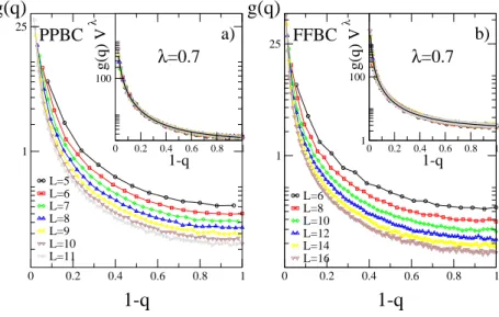
FIG. 1. g(q) versus 1 − q for the PP (left panel) and FF case (right panel) for different lattice sizes L = 5 − 11 (PP) and L=6-16 (FF) from top to bottom. In both insets we plot the scaling function g(q)Vλ_{versus 1 − q with λ = 0.7.}

In Fig. 1 we show g(q) = V

2gvas function of q for different sizes in the PP and FF cases. We can clearly see that there

are excitations of all possible sizes but, as discussed in the paragraph following (9), the typical ones which dominate by far are single spin excitations. To have a rough idea of the number of rare samples giving large scale excitations let us say that nearly half of the total number of samples have one-spin lowest excitations, whereas less than 10% of the samples have lowest excitations with overlap q in the range 0 − 0.5. This disparity increases systematically

with size. For the lattice sizes explored the typical number of large-scale droplets is in the range 104_{− 10}5 _{which is,}

indeed, quite good to have a good sampling of the sector corresponding to large scale excitations. A detailed analysis

of the shape of gv reveals that it has a flat tail for large-scale excitations and a power-law divergence for finite-size

g(q) = 2 Vλl µ A + B (1 − q)λl+1 ¶ . (23)

As shown in the insets of Fig. 1 a good collapse of the scaling function is obtained with the effective exponent λeff

l ' 0.7

for both PP and FF cases. We also plot the line resulting from the fit of (23) with numerical data with the following values for A and B: PPBC: A = 1.55(3) and B = 0.777(3); FFBC: A = 2.02(3) and B = 0.85(1). Note that the fit is

excellent and is hardly distinguishable from the points. The value of λlis compatible with the one obtained by fitting

the average size with the expression (10) with the addition of a constant term to account for the small-V behavior,

v = C1+ C2V1−λ. The same exponent λl can be estimated by measuring the ratio g(V /2)/g(1) ∼ D1+ D2V−1−λ.

In both cases we get an effective exponent λeff

l = 0.70(5) as best fitting value.

However these different estimates of λlare strongly affected by finite-volume corrections (FVC). To evidence them

we have estimated an effective L dependent λeff

l (L) exponent by relating the average excitation size at consecutive

sizes and using relation (10),

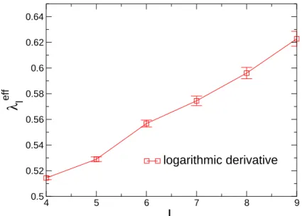
λeff l (L) = 1 − 1 d log³v(L+1)_v(L) ´ log³L+1 L ´ . (24)

In Fig. 2 we show λeff

l (L) in the range L = 4 − 11 for the PP case. As we can appreciate there is a systematic increase

of the effective exponent as we go to large volume sizes without any tendency to saturate. This proves that FVC in

our measurements are still big and the estimate λeff

l used to collapse the data in Fig. 1 is still far from the asymptotic

exact value. 4 5 6 7 8 9

L

λ

logarithmic derivative

FIG. 2. Effective lowest droplet exponent λeff

l versus L for the PP case, computed using logarithmic derivatives.

After having discussed the gv we jump now to discuss the scaling behavior of the energy gap distribution ˆPv(E)

and its average P (E). In Fig. 3 we show P (E) (main figure and inset a) and ˆPv(E) (inset b) for the PP case. Similar

results are obtained for the FF and FP cases. Quite remarkably, as was already anticipated in (11), the RESD scenario

holds as the distribution ˆPv(E) does not depend on the size v of the excitation (see inset b in Fig. 3), hence both

large and finite-size excitations are described by the same gap distribution.

In the main figure we can see how the width of distribution P (E) progressively shrinks to 0 as L increases. Moreover, the P (E) has an exponential shape. This is shown in the inset a) of Fig. 3 where we plot P (E) in log-normal scale. Nonetheless, a detailed examination of the tails of P (E) reveals some deviations from linearity. In Sec. VI we discuss the origin of these deviations. We anticipate, though, that they are consequence of the strong FVC in the range of sizes investigated. In that inset we also verify the scaling ansatz (13) by showing the best data collapse for P (E)

obtained with an effective exponent θeff

l ' −1.7(1). This is very far from the expected value θl= −2 discussed in the

preceding Sec. II C and in the Appendix A. A calculation of the moments of P (E) (13) for different values of L shows that there are also strong sub-dominant corrections to the leading scaling (13) that result in corrections as large as

0 10 20 30

E/ L

E

P(E)

Ε

P

(E)

FIG. 3. Gap distribution P (E) versus E for different lattice sizes in the PP case. In inset a) scaling obtained from the ansatz (13) with θeff

l = −1.7(1). In inset b) we show the ˆPv(E) for different excitation sizes (q = 0.5, q = 0) for a lattice size L = 10.

Note that the distribution is independent of the size of the excitation.

Again, to manifest the magnitude of FVC in θl we have evaluated E(L), the first moment of ˆP (E), obtained by

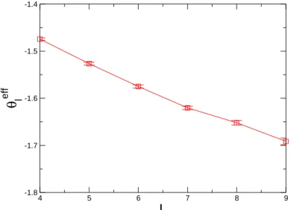
averaging the lowest gap over all possible droplet sizes for different lattice sizes in the range L = 4 − 11. We have estimated an effective L-dependent exponent by means of the following expression,

θeffl (L) =

log³E(L+1)_E(L) ´

log³L+1

L

´ . (25)

The results are shown in Fig. 4 for the PP case. Again, as for λeff

l (see Fig. 2), we observe that the estimated value for

θeff

l systematically changes with size showing that, for the sizes we have explored, we are still far from the asymptotic

regime. 4 5 6 7 8 9

L

θ

FIG. 4. Effective droplet exponent θeff

l versus L for the PPBC case, computed using logarithmic derivatives (see text).

We can summarize the results of this section saying that both lowest droplet exponents (LDEs) λl and θl display

strong systematic finite-volume corrections (FVC). In principle, without further elaboration, it is difficult to give an accurate estimate for the thermal exponent θ using (18). An alternative estimate for the exponent θ could be defined

f (q ≤ 1/2) ∼ V g(0) ∼ 1/Vλl−1 _{∼ L}d(λl−1)_{∼ 1/L}θ_{, (26)}

where we have used θl= −d (19). Although (26) yields estimates for θ, again these are affected by strong

finite-volume corrections. In the range of sizes studied in this paper, and using (26) we get θ ' −0.6 quite far from the asymptotic value reported later in Secs. IV and V. How can we go further and estimate θ in a safer way? In the next two sections we shall answer this question.

IV. A GOOD ESTIMATE OF THE LOWEST DROPLET EXPONENTS

An interesting aspect of the effective L-dependent exponents shown in Figs. 2 and 4 is that, while their FVC are

large, their corrections are of opposite sign. While λeff

l (L) increases with L, θleff(L) decreases. As they have to be

added to get θ according to the relation (18) their finite-volume corrections cancel out to a certain degree. If we

combine the two estimates for the best data collapse given in the previous section (λeff

l = 0.70(5), θeffl ' −1.7(1))

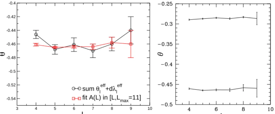
we obtain θ ' −0.3(2) which is very close to the DW value in average. However, this estimate is too pessimistic. A better route would be to use the two LDEs estimated from (24),(25) and adding them according to (18)

θeff_{(L) = θ}eff

l (L) + dλeffl (L) . (27)

In Fig. 5 (left panel) we show the value of θ obtained in this way. Note that the value of the thermal exponent θ has

negligibleFVC but relatively large statistical fluctuations with L.

A better, albeit related, way to estimate θ is the following. Instead of independently finding out λland θl we look

for an estimator which depends on the appropriate combination of the two exponents θ = θl+ dλl. The simplest

quantity which satisfies this requirements is given by the combination,

A(L) = LdE(L)

v(L) . (28)

Since E(L) ' Lθl _{and v(L) ' L}d(1−λl)_{, using (18) we obtain A(L) ∼ L}θ_{. To estimate the value of θ we follow two}

different routes: 1) We use (25) by replacing θeff

l (L) → θeff(L) and E(L) → A(L). By definition, this procedure gives

exactly the estimate (27) shown in the left panel in Fig. 5. 2) A more stable estimate can be obtained from a fit of

A(L) versus L, with data in the range [L, · · · , Lmax = 11] (for the PPBC case). This is shown in the left panel of

Fig. 5 together with the previous estimate (27) and also in the right panel of Fig. 5 but there compared with the

effective exponent θDW obtained from domain-wall calculations. Our best value for θ is

θ = −0.46(1) . (29)

This value is very close to the finite-temperature (Monte Carlo or transfer matrix) estimates θT F = −0.48(1)19 but

certainly smaller than the domain-wall value θDW = −0.2857,8. Our estimate for θ is compatible with the other

possible value θT F obtained by other methods as discussed in Sec. I but is certainly inconsistent with the value

obtained with other methods with results closer to the DW estimate.

3 4 5 6 7 8 9 10 L -0.54 -0.52 -0.5 -0.48 -0.46 -0.44 -0.42 -0.4

θ

sum θ_leff+dλ_leff fit A(L) in [L,L_max=11]

FIG. 5. Exponent θ for the PPBC case. Left plot: θ exponent versus L obtained from two methods. Method 1: using (27). Method 2: using the more stable estimate fitting (28) over a given range of L values (see text). Right plot: Domain-wall exponent (top) and θ exponent (bottom) estimated by the second method as explained in the text and plotted as a function of L.

All these estimates strongly support the inequality θ = θT F < θDW. However, one cannot exclude a situation where

the present tendency of the data gets modified and θ → θDW in the large-L limit30. We have already explained in

Sec. II C that θl must converge to −2 in the large volume limit implying the relation (19). Introducing our estimate

(29) in (19) we get,

λl= 0.770(5) . (30)

A convincing proof of the correctness of the values (29,30) requires proving that the estimate (24) converges to the value (30) when L → ∞. In the next section we present an aspect-ratio analysis to evidence that the estimates (29),(30) are correct in the large L limit.

V. ASPECT-RATIO ANALYSIS OF THE LOWEST DROPLET EXPONENTS

In this section, we present some additional data obtained via an aspect-ratio analysis (ARA). This analysis has

been proved to be very useful to extract the value of the domain-wall exponent θDW by generating domain walls in

rectangular lattices M × L with different aspect ratios M/L24,27_{. It has been found that, in the limit of large aspect}

ratio, the value of θDW for Gaussian spin glasses is largely independent of the boundary conditions. We have seen

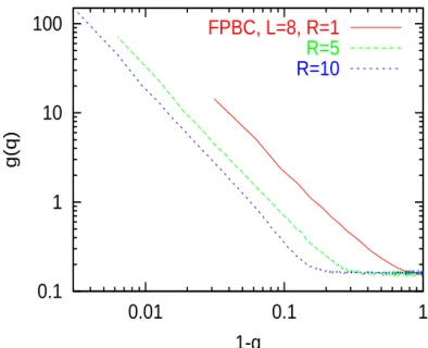
in Sec. III that our measurements on squared lattices of size L × L mix small excitations with large ones so one does not have a clear-cut separation in the statistical distribution between the two different regimes v ∼ O(1) and v/V ∼ O(1). Our main motivation here is to show that, by investigating large aspect-ratios, we can separate these two different scaling regimes. We made our measurements on systems of size L × M , with M = LR >> L where R ranges from 1 up to 10. We have investigated different types of boundary conditions: periodic boundary conditions in both directions (PPBC) and periodic boundary conditions in the L direction with free boundary conditions in the M direction (FPBC).

In Fig. (6), we display the data for g(q) versus 1 − q (8) for the FPBC case for L = 8 and R = 1, 5 and 10. One can clearly see that the behavior of the distribution g(q) drastically changes as one increases R. Indeed, as we have already seen in Sec. III and in (5), (6), (8), for R = 1 it is very difficult to separate the region of small excitations (a scaling

region with g(q) ' _(1−q)1_λl+1) from the one of large excitations (a constant q-independent contribution g(q) ' _V1_λl).

The main advantage of separating these two regions is that one can fit directly each of them. This yields two separate

measurements of the LDE λlin addition to the estimate (10) obtained from the L dependence of the average size of

the excitations.

0.1

1

10

100

0.01

0.1

1

g(q)

1-q

FPBC, L=8, R=1

R=5

R=10

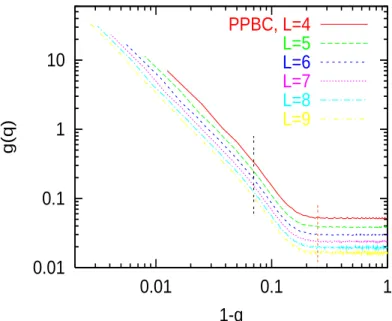
In Fig. (7), we show g(q) versus 1−q for R = 10 for various linear sizes L and for the PPBC case. These distributions have been obtained by running a large number of samples ranging from 10 million of samples for L = 4 down to 5 million for the largest size L = 9. We have also inserted in the figure two vertical lines which indicate the limits for the range of values we have chosen for the fits of the scaling behavior of the finite-size excitation sector (1 − q ≤ 0.07) and for the constant contribution corresponding to large scale excitations (1 − q ≥ 0.25). We have chosen these values for the following reasons. First, as one can clearly see in Figs. (6,7), the scaling region for small excitations survives

up to excitation sizes v ' L × L. This size provides a threshold value for the overlap qth below which the simple

scaling g(q) ' 1

(1−q)λl+1 does not hold anymore,

1 − qth = 1 − (1 − 2v V ) ' 2L2 RL2 ' 2 R . (31)

An second, there is a crossover region around q ' qth. A careful look at Fig. (7) shows that the scaling region for

small excitations ends around 1 − q ' 0.07. At this value, one observes a change of the slope of the curves just before entering the regime of large excitations where g(q) becomes q independent. For 1 − q ≥ 0.25, the curves are rather constant and the result of a fit does not depend much on the choice 1 − q = 0.25. This second threshold value is indicated as the rightmost vertical bar in Fig. (7).

0.01

0.1

1

10

0.01

0.1

1

g(q)

1-q

PPBC, L=4

L=5

L=6

L=7

L=8

L=9

FIG. 7. g(q) versus 1 − q for the PPBC case for R = 10.

In Fig. (8), we show the estimated values of effective lowest droplet exponent λeff

l obtained in three different ways.

The first estimate has been obtained by averaging the volume of all excitations for different lattice sizes as explained in Sec. III and then taking a logarithmic derivative, see (24). The second estimate has been obtained by considering the large excitation sector (1 − q ≥ 0.25) and its L, R dependence:

g(q) ' (RL2)−λl _{. (32)}

Averaging the excitation volume within this sector (1 − q ≥ 0.25) and using again the corresponding logarithmic

derivatives as in (24) yields the second estimate. The third estimate for λl is obtained from a direct fit of g(q) for

small values of 1 − q :

g(q) ' (1 − q)−1−λl _{. (33)}

This third method is in fact the most direct one since it can be done for each size L (while the other two estimates

require a fit using data from two different lattice sizes L and L0_{). The first conclusion that we learn from Fig. (8) is that}

the ARA produces a great improvement on the estimated values of the exponent λl. The most stable measurement is

the third estimate obtained by fitting the small-size spectrum of the excitations. In that case, λeff

l is nearly constant

λl= 0.77(1) (34)

in excellent agreement with the result (30) of the previous section.

FIG. 8. Effective lowest droplet exponent λeff

l versus L for the PPBC case for R = 10. We represent the values of λ eff l

obtained from fitting the distribution of g(q) for small excitations (solid line), for large excitations (short dashed line) as well as the value obtained by fitting the average size of excitations (dotted line).

Moreover, one also observes in Fig. (8) that the two other estimated values for λeffl , obtained with the first and second

methods, are strongly correlated. This shows that finite-volume corrections, which are expected to affect the value of the exponent obtained from the analysis of large-size excitations, does affect also the value of the exponent obtained by averaging over the whole spectrum. In addition, we also observe that the ARA for large R strongly decreases the

magnitude of finite-volume corrections. While on a square geometry, the effective exponent λeff

l obtained from the

average size of excitations took values in the range 0.52 − 0.62 (see Fig.(2)), with the ARA, we obtain for the same exponent values in the range 0.64 − 0.72, which are much closer to the expected asymptotic value 0.77(1).

-1.9

-1.85

-1.8

-1.75

-1.7

-1.65

-1.6

-1.55

-1.5

-1.45

-1.4

-1.35

4

5

6

7

8

9

10

11

12

θ

L

FPBC

PPBC

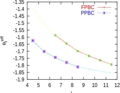
FIG. 9. Effective exponent θleff obtained via a logarithmic derivative for the PPBC and the FPBC. We also plot best fit

curves which converge to θeff

l (L → ∞) = −1.96(6) for the PPBC and to θ eff

The same conclusion holds for the lowest droplet exponent θl. In Fig. (9), we show the effective exponent θeffl

obtained by evaluating the logarithmic derivative as in (25). Note that finite-volume corrections are much smaller than with the squared lattices and as a result, the value of the effective exponent converges much faster to the expected

value −2. Using a fit of the form θleff(L) = θleff(∞) +Lcstα, one gets θ

eff

l (∞) = −1.96(6) for the PPBC, the best fit

being also represented in Fig. (9). In this figure, we also show the same exponent obtained for the FPBC, where the

best fit yields the asymptotic value θeff

l (∞) = −2.12(11). In both cases the fitting value we obtain for the exponent

is α ' 1. Note that the asymptotic values for θeff

l are well compatible with our prediction of Sec. II C, θl= −2 (see

also the heuristic argument in Appendix A).

VI. FINITE-VOLUME CORRECTIONS (FVC) AND THEIR RELATION TO THE STATISTICS OF EXTREME VALUES

What is the origin of these strong finite-volume corrections? Intuitively it is not difficult to find an explanation

for the strong systematic finite-volume corrections in the lowest droplet exponent θl. As the word lowest indicates,

these exponents describe the statistical distribution of droplet excitations which are at the tail of the energy gap distribution that includes all possible high energy levels. As the volume of the system increases there is more available space to find excitations with lower energy gap. This implies that there is more probability to find a lowest droplet

with an energy smaller than a given threshold value E∗. As this probability systematically increases with L for all

samples, θeff

l (L) must be a decreasing function of L. This is in agreement with what we have found. The behavior of

λeff

l (L) is more difficult to establish. By the same token, although there is more available space for droplets we expect

that different droplet sizes increase or decrease their relative probability in a non-trivial way making difficult to guess

how the exponent λeff

l (L) systematically changes with L.

0 2 4 6 8 10

h

p

(h)

L=4

L=5

L=7

L=8

L=9

L=9

L=10

L=11

L=12

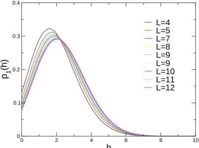
FIG. 10. Local-field distribution for different lattice sizes with FFBC boundary conditions.

To understand the origin of finite-volume corrections in the value of θl we have focused our attention on the

behavior of the upper bound exponent θ1l describing the statistics of the lowest one-spin excitations as described

in the Appendix A. The gap distribution corresponding to these excitations can be obtained from the local-field distribution evaluated at the ground state. We have numerically computed this distribution for different sizes, the results are shown in Fig. 10. As discussed in the appendix A, the local-field distribution has a finite weight at zero field and is a self-averaging quantity. As the local field distribution is self-averaging, the probability distribution for

the lowest one-spin excitations corresponds to the extreme value statistics of the local-field distribution p1(h) where

h stands for the local field which we assume to be positive as the gap is given by its absolute value (the subindex 1

is used to stress that this distribution describes energy gaps for one-spin excitations only). If P1(h) stands for the

probability distribution of the smallest local-fields, then P1(h) can be easily related to p1(h) by standard probability

arguments (see for instance,28_{). Although the argument is very general, here we apply it to one-spin excitations. For}

a given sample, the lowest value h is selected as the minimum value among all the possible V local fields hi at each

P1(h) = V p1(h)(1 − Z ∞ h p1(h0)dh0)V −1= − ∂ ∂h à Z ∞ h p(h0)dh0 !V (35) which accounts for all possible ways the value h coincides with the minimum value obtained among all different V

local fields distributed according to the p1(h). The last identity shows that P1(h) is normalized. This probability can

be explicitly worked out in the large V limit,

P1(h) = −

∂

∂hexp [−V g1(h)] = V g1(h) exp [−V g1(h)] . (36)

Up to second order in h the function g1(h) is given by,

g1(h) = p1(0)h +

p0

1(0) + (p1(0))2

2 h

2_{. (37)}

From (36) we immediately learn that the gap distribution is an exponential with a sub-leading Gaussian correction

whose magnitude decreases as 1/V . Actually, plotting P1(h)/V as function of the scaling variable x = hV one gets,

P1(h) V = g 0 1(x/V ) exp · −xp1(0) −p 0 1(0) + (p1(0))2 2V x 2 ¸ . (38)

In the large V limit g0

1(x/V ) → p1(0) and the coefficient in front of the Gaussian correction goes asymptotically to

zero, therefore the distribution P1(h) converges to an exponential as expected,

P1(h) = V p1(0) exp¡−V p1(0)h¢ (39)

in agreement with the scaling relation (13). We can now understand the deviations from the pure exponential behavior discussed in Sec. III in the context of the inset a) shown in Fig. 3. They are simply consequence of the finite-volume corrections of the extreme values of the gap distribution for all energy levels (and not only one-spin excitations as we are discussing here). So one could imagine to compute for a given sample the first V energy gaps corresponding to

the first V excitations. We also assume that the resulting distribution pall(E) is self-averaging in the large volume

limit (as it is the local-field distribution p1(h)). The lowest energy distribution constructed by taking the minimum

value of the gap E for each sample yields the extremes distribution Pall(E) defined in (13) (from now on we will drop

the subindex ’all’ in Pall(E) as it coincides with the P (E) defined in (13). Also the subindex ’all’ for the pall(E)

will be dropped). In fact, the parameters p(0), p0_{(0) characterizing this distribution can be obtained from the P (E)’s}

shown in Fig. 3. To evaluate them, the best way is to analyze the cumulative distribution P(E) = R∞

E d E0P (E0)

which from (35) we can assume to be P(E) = exp[−V gall(E)]. Thus we can fit P(E) with an exponential with

Gaussian corrections A exp[−Bx − Cx2_{/2] whose fitting parameters are related to p(0) and p}0_{(0). The best fits yield}

the following values p(0) ≈ 0.2 and p0_{(0) = 0.3.}

4 6 8 10 12

L

θ

v=1 FFBC

lowest excitation FFBC

FIG. 11. Effective droplet exponent θeff

l versus L for the FFBC case, computed using logarithmic derivatives (see text). We

show the exponent obtained for one-spin excitations (v = 1) in comparison to the one obtained from the whole distribution of gaps.

Coming back to our original goal we discuss now the finite-volume corrections for the estimate θeff

l , as shown in

Fig. 4. From the distribution (36) describing the whole spectrum of excitations we can express the effective exponent (25) for L >> 1 as,

θleff(L) =

∂ log¡E(L)¢

log(L) . (40)

The computation of E(L) is quite straightforward as it is given by the simple relation, E(L) = Z ∞ 0 EP (E)dE = Z ∞ 0 exp³− V g(E)´ (41)

where we have used (36) plus an integration by parts. The integral, up to second order in 1/V yields,

E = 1 V p(0)− p0_{(0) + (p(0))}2 V2_(p(0))3 + O ³ 1 V3 ´ . (42)

Inserting this result in (40) we finally get,

θleff(L) = −d + d V¡1 + p0(0) (p(0))2¢ + O ³ 1 V3 ´ . (43)

This shows that θeff

l (L) approaches −d from below (as p0(0) is positive). On the other hand the magnitude of the

finite-volume corrections can be pretty large if _(p(0))p0(0)2 >> 1. For instance, if one takes the results obtained from

the analysis of one-spin excitations one gets p1(0) ' 0.069, p01(0) ' .125 yielding

p0 1(0)

(p1(0))2 ' 27. which is indeed large.

Inserting these values in (43) we obtain an estimation for θeff

l (L = 12) = −1.65 in good agreement with numerical

results (see Fig. 11).

If we insert the previous estimated values for the whole spectrum of excitations extracted from the P (E)’s in Fig. 3,

we obtain _(p(0))p0(0)2 ' 7.5. From (43) it follows that θ_leff(L) ' −2(1 − 7.5/V ), which for L = 11 yields θeff_l = −1.87. All

in all, the magnitude of the effective exponent θl is well compatible with the reported value θeffl used in the inset a)

in Fig. 3 for the PP case. Note that the FVC corrections to θeffl obtained from the local-field distributions in the FF

case are much larger than FVC corrections in the PP case in agreement with ARA results (see Fig. 9). From this

analysis it becomes clear that to significantly reduce the magnitude of the finite-volume corrections in the value of θl

(let us say θl' −1.95), we would need larger volumes beyond 20 × 20.

VII. COMPACTNESS OF THE LOWEST ENERGY DROPLETS.

One intriguing question about the droplet excitations concerns their topological properties. Kawashima and Aoki20

have argued that droplet excitations are not compact. Instead, their volume has a fractal structure as the number of lattice points included in the droplet scales with its spanning length (which is a measure of the length scale of the droplet) with an exponent smaller (around 1.80(2)) than the dimension of the system (2).

To answer this question we have computed the surface, i.e. the perimeter P , of all lowest droplets. The relation between the average perimeter as function of the size v of the excitation depends on both the fractal dimension of the

surface or perimeter ds and the volume dv of the lowest droplets. dsand dv can be defined in terms of the spanning

length l of the droplet which can be defined in different ways. For example, one could use the gyration radius, the average distance between the sites contained in the cluster, or the maximum distance among the sites of the cluster. As the typical length scale of our lowest droplets is small, l ' 10, we have not attempted to estimate it as this can strongly depend on the precise definition of the spanning length. Here, we restrict ourselves to investigate the perimeter-volume dependence. In terms of the spanning length l the surface fractal and volume fractal dimensions

ds, dv of the droplets are defined as,

l ∼ Pds1 (44)

l ∼ vdv1 (45)

P ∼ vdsdv . (46) In Fig. 12 we show P (v) as a function of v for different lattice sizes. As can be seen, FVC are important for large volumes. However, there is an enveloping curve that is independent of L for small volumes and spans a progressively increase range of volumes as L increases. This enveloping curve is excellently fitted (continuous curve) by the scaling relation (46) and yields an estimate,

ds

dv

' 0.632(2) (47)

consistent with the results reported by Kawashima and Aoki ds

dv = 0.61(1) obtained with a completely different

method. 0 10 20 30 40 50 60

v

P

L=7

L=8

L=9

L=10

fit y~v

FIG. 12. Perimeter (P ) of the droplet versus its volume (v). The solid line corresponds to the fit (46) with ds/dv= 0.632(2).

VIII. CONCLUSIONS

We have shown that a proper description of low-temperature properties in two-dimensional Gaussian spin glasses

can be done in terms of the lowest droplet exponents (LDEs) λland θldescribing the spectrum of lowest excitations.

λl describes the spectrum of sizes of the lowest energy droplets, while θl describes the typical energy cost of these

lowest droplets whatever their size. Assuming that θl = −d one concludes that the LDE λl fully characterizes the

spin-glass phase. Although independent numerical estimates of θl and λl show strong finite-volume corrections, the

thermal exponent θ = θl+ dλlcan be well estimated giving the results (29), (30)

θ = −0.46(1) λl= 0.770(5). (48)

unambiguously showing that θ < θDW = −0.287(4)27. Our estimates (48) have been confirmed via an aspect-ratio

analysis which provides estimates much less influenced by finite-volume corrections. Moreover, the result θl = −2

(that is believed to be correct for spin glasses with coupling distributions with finite weight at zero coupling, see the Appendix A) has been numerically confirmed by the aspect-ratio analysis. To sum up, McMillan’s excitations are not the typical low-lying excitations and our approach offers a new and independent way to estimate the thermal exponent θ without the need to generate typical low-lying excitations by looking at the new ground state of the system after perturbing it.

We think that discrepancies on the value of the thermal exponent θ reported by comparing non-perturbative methods (such as finite-temperature transfer-matrix calculations and the present lowest droplet analysis) with perturbative

methods such as domain-wall calculations (or perturbations induced by introducing a coupling term in the energy

function that induces a large-scale excitation) are serious enough to be taken as a clear indication that our knowledge of the low-temperature properties of the 2d GISG is still inadequate. In this direction we want also to recall the issue

of multifractality and the possibility that different exponents could describe the zero-temperature critical point. Is this really possible? Well, to our knowledge no exact result precludes this possibility and, although purely speculative at the present stage, one should seriously think about it. Altogether, the present analysis suggests that the excitations in 2d GISG are very different from the compact droplets proposed in the context of the droplet model. If this were true, the implications of the 2d studies in larger dimensions could be important. There are many routes that can be followed to understand better what is going on and the origin of this discrepancy. Certainly, with the outstanding accuracy of present algorithms to compute ground states in 2d, it would be very interesting to revisit again the analysis of the statistics of the large scale excitations generated by imposing a uniform magnetic field. “Old” results

by Rieger et al.8 _{give an estimate for θ that is compatible with our estimate rather than to the domain-wall estimate.}

This would be an independent check of our values, but using a perturbation method with an appropriate neutral

observablesuch as the global magnetization as has been explained in Sec. I before (1).

The proposed method may appear venturesome as, to our present knowledge, there is no numerical study in the field

along this line of research. However, as explained in Sec. I, recent studies on the disordered Anderson model12 _have

revealed that the analysis of the lowest excitation provides a good description of the localized phase. More studies are certainly required to understand better the reliability of the present method to investigate the critical properties of spin glasses. One disadvantage of our approach is that a huge number of samples is needed to reasonably sample large-scale excitations. However, as we saw in Sec. V, the behavior of the g(q) for small 1 − q can be extracted with a modest number of samples. The advantage, as has been already stressed in Sec. I, is that we do not introduce any external perturbation to generate the excitations.

Finally, we want to comment on the extension of this approach to other models. Of course, the immediate extension one could think of is the 2d ±J model. However, the analysis of this model appears quite troublesome. This model does not have a continuous gap distribution but a discrete one that introduces further complications. As the ground state is not unique one has to redefine the full analysis to properly define the spectrum of lowest excitations. The discreteness of variables could have some unexpected effects in the present approach as seems to happen also with

domain-wall calculations22,27_{. It is more natural to extend the research to other models such as 2d ISG with other}

continuous coupling distributions without gap (e.g. characterized by P (J) ∼ |J|α_{for |J| → 0), Migdal-Kadanoff spin}

glasses (where both the ground state and the first excitation could be feasibly found with an appropriate algorithm), Gaussian spin glasses beyond d = 2 (where unfortunately, algorithms are much less effective than in 2d as the finding of the ground state becomes a NP complete problem) and finally mean-field spin-glass models where the zero temperature exponents are known and maybe the spectrum of lowest excitations could be analytically tackled. Preliminary results

in this case29 confirm that the present analysis describes pretty well the data for rather small sizes. We are pretty

confident that, in the near future, new results and evidences will finally resolve this interesting problem.

APPENDIX A: HEURISTIC PROOF OF THE IDENTITY θL= −D

In this appendix we show that θl = −d. In what follows we do not attempt to present a rigorous proof but we

content ourselves to present an heuristic argument. The argument has two parts: first we show that −d is an upper bound, next we show that the upper bound is the exact value. For the upper bound the argument is well known and goes as follows. Consider the ground state and all possible one-spin excitations. Because one-spin excitations are not necessarily the absolute lowest ones, the statistics of the lowest one-spin excitations must yield an upper bound θ1

l for the value of θl, θl ≤ θ1l. The statistics of the lowest one-spin excitations is determined by the behavior of

the ground-state local field distribution p(h) in the limit h → 0. If p(h) is self-averaging and p(0) is finite (in the

large-volume limit) then the statistics of the lowest excitations must be governed by the exponent θ1

l = −d. Although

we do not know a precise mathematical proof of the statement that p(0) is finite, it looks quite intuitive16_{. In any}

short-range system with a frustrated ground state and a coupling distribution with finite density at zero coupling, we may expect a finite probability to find a cage containing a spin coupled to its neighbors by a set of weak bonds which produce a vanishing net local-field acting on that spin. This argument should generally hold for d ≥ 2. Moreover, as

its name indicates, the local-field distribution is a local observable. An argument `a la Broutproves that it should be

self-averaging as all possible local field values are realized across the whole lattice1_{. The next part of the argument}

consists in proving that an identical upper bound is valid by considering excitations with size strictly larger than 1 but finite. The upper bound derived for the one-spin excitations must necessarily hold for finite-size excitations beyond one-spin excitations (for instance two-spins, three-spins and so on) as the gap corresponding to the finite-size

excitations can always be written as a linear combination of a finite number of local fields with coefficients which depend on the ground state configuration. It is easy to verify that the aforementioned properties of the local-field distribution p(h) imply that the new gap distribution has a finite weight at zero gap and is self-averaging. This argument however cannot be extended to large-scale (with v ∼ V ) excitations in a straightforward way because the distribution for the corresponding gap distribution corresponds to an infinite sum of terms in the V → ∞ limit.

However once we argue that θl is an upper bound valid for all finite-size excitations it can be concluded that this

upper bound must coincide with the exponent θldescribing the probability of the absolute lowest excitations. From (4)

the fraction of large scale excitations v → V is given by V gV = _V1λ. In general λ > 0 so this fraction vanishes

2 _in

the infinite-volume limit and finite-size excitations determine the result θl = −d as they dominate the spectrum of

lowest excitations. Moreover, if large-scale excitations yield a different value for θl this would imply that boundary

conditions could affect the value of the thermal exponent. That would be quite unusual as this would mean that the exponents of the T = 0 fixed point would depend on the boundary conditions.

APPENDIX B: TRANSFER MATRIX ALGORITHMS

In this appendix, we will briefly explain how we determine the ground state and the first excited state. We will work on a square lattice of size L × L. The energy associate to a configuration of spins S(i, j) with a fixed configuration of

disorder Jx_{(i, j) and J}y_{(i, j) is}

E = X

i=1,L−1

X

j=1,L

Jx(i, j)S(i, j)S(i + 1, j) + X

i=1,L

X

j=1,L−1

Jy(i, j)S(i, j)S(i, j + 1) (B1)

+B1 X j=1,L Jx_{(L, j)S(L, j)S(1, j) + B} 2 X i=1,L

Jy_{(i, L)S(i, L)S(i, 1) ,}

where B1and B2correspond to the choice of boundary conditions. Here we will consider three cases : Periodic-Periodic

boundary conditions (PPBC) with B1 = B2 = 1; Free-Periodic boundary conditions (FPBC) with B1 = 1; B2 = 0

(or equivalently B1= 0; B2= 1) and Free-Free boundary conditions (FFBC) B1= B2= 0. We will only consider the

case with a Gaussian distribution of the bond disorder Jx_{, J}y_{. To determine the ground state and the first excited}

states, we proceed as follow: we start by associating a weight for each configurations of spins in the first row of the lattice S(1, 1), S(1, 2), · · · , S(1, L):

W (S(1, 1), S(1, 2), · · · , S(1, L)) = B2Jy(1, L)S(1, L)S(1, 1) +

X

i=1,L−1

Jy(1, i)S(1, i)S(1, i + 1) . (B2)

Next, we start iterating the transfer matrix using a sparse-matrix factorization31_{. The first iteration gives}

W1(S(1, 2), · · · , S(1, L), S(2, 1)) = maxS(1,1)[Jx(1, 1)S(1, 1)S(2, 1) + W (S(1, 1), · · · , S(1, L))] . (B3)

Since we are also interested in the first excited state, we define the second largest weight:

W2(S(1, 2), · · · , S(1, L), S(2, 1)) = minS(1,1)[Jx(1, 1)S(1, 1)S(2, 1) + W (S(1, 1), · · · , S(1, L))] . (B4)

In the following, we will use the simplified notation

W (i, j) ≡ W (S(i, j), · · · , S(i, L), S(i + 1, 1), · · · , S(i + 1, j − 1)) . (B5)

Thus eqs.(B3,B4) become

W1_{(1, 2) = max}

S(1,1)[Jx(1, 1)S(1, 1)S(2, 1) + W (1, 1)] (B6)

and

W2_{(1, 2) = min}

S(1,1)[Jx(1, 1)S(1, 1)S(2, 1) + W (1, 1)] . (B7)

2_{This fractions is finite only in d = 1 where λ = 0. But this case is trivial as the surface of large scale droplets in d = 1 only}