Design of a low-mass high-torque brushless motor for application in quadruped robotics

Design of a Low-Mass High-Torque Brushless

Motor for Application in Quadruped Robotics

by

Niaja Nichole Farve

B.S., Electrical Engineering, Morgan State University, 2010

Submitted to the Department of Electrical Engineering and Computer

Science

in partial fulfillment of the requirements for the degree of

Master of Science in Electrical Engineering and Computer Science

MASSACHUSETTS IN

at

the

MASSACHUSETTS INSTITUTE OF TECHNOLOGY

JUL

0 1 201

June 2012

_LIBRARIE

@

Massachusetts Institute of Technology 2012. All rights reserved.

ARCHIVES

Author

₍

_{.. . .}

... ...

Depar

en Uoofiectrical Engineering and Computer Science

May 23, 2012

/1

///i

/

Certified by ...

Professor of Electrical

.. ... . ... .'

I

Jeff rey H. Lan

Engineering and omputer Science

Thesis Supervisor

A ccepted by ...

...

C r Dmee

i A. Kolodziejski

Chairman, Department Committee on Graduate Students

Design of a Low-Mass High-Torque Brushless Motor for

Application in Quadruped Robotics

by

Niaja Nichole Farve

Submitted to the Department of Electrical Engineering and Computer Science on May 23, 2012, in partial fulfillment of the

requirements for the degree of

Master of Science in Electrical Engineering and Computer Science

Abstract

The Biomimetic Robotics Group is attempting to build the fastest quadruped robot powered by electromagnetic means. The limitations in achieving this goal are the torque produced from motors used to power the robot, as well as the mass and power dissipation of these motors. These limitations formulate the need for a low-mass high-torque low-loss motor. This thesis outlines the process of designing a permanent-magnet synchronous motor that meet the goals of the robot while mini-mizing the total mass. The motor designed from this thesis is compared to motors currently used by the Group when quantifying improvements made. In the process of achieving the goal, a design was formulated using fundamental electromagnetic prin-ciples. This design was then tested using finite element analysis. The final design was fabricated in house and wired by hand. The fabricated motor was tested to quantify key performance parameters such as peak cogging torque, peak motor torque, and thermal time constant under robot conditions. The motor designed by this thesis was able to produce more torque than the current motor being used by the Biomimetic Robotics Group, by a factor of 1.6, while decreasing the mass by 23%. A lower than desired packing factor was achieved since the motor was wired by hand resulting in a higher power dissipation and lower than expected motor torque. This design will be used in the quadroped robot after improvements are made to the cogging torque and packing factor.

Thesis Supervisor: Jeffrey H. Lang

Acknowledgments

"Gratitude is a quality similar to electricity: it must be produced and discharged and used up in order to exist at all"

~William Faulkner

I am beyond grateful for the never ending number of friends and family present in my life that encourage and inspire me everyday. Without which every mountain climbed would have been unfathomably higher. I wish I could name every person, but I think the list would exceed this thesis.

I am especially grateful for my mother, role model, and best friend. You have pushed me to try even when success seemed impossible. You have always been there to help fix my problems and see the rainbow in the storm. I hope to one day become half the mother you have been to me.

MIT would not have been as enjoyable without the man in my life that has been unbelievably understanding and encouraging, Omar. The friends I left at Morgan have also sporadicly brightened my weekends at MIT with their visits, reminding me of what great life long friends I have made. Likewise, new friends made here at MIT have helped to put things in perspective and gave my a small group where I feel like "I belong". Thank you for always being there to give me a reality check and helping me enjoy life.

I don't think I could have possibly found a better adviser. Thank you Jeff for being beyond patient and spending so much of your precious time with my endless questions.

I am also grateful to this institution as well as the RLE lab for giving my the chance to succeed in such a rigorous and challenging environment. I have grown in ways unimaginable due to my experience here.

This work was funded by a Brookhaven National Laboratory Masters GEM Fel-lowship, and the DARPA grant 019719-001. The Biomemtic Robotics Group also provided funding and a tremendous amount of support. I am grateful for each of these resources and would not have been able to complete this thesis without this

Contents

3.3 Mass and Rotor Inertia Calculations . . . . 43

3.4 Resistance and Inductance Calculations . . . . 43

4 Fabrication 49 4.1 Hardware ... 49 4.1.1 Laminations . . . . 49 4.1.2 M agnets . . . . 54 4.1.3 W ire . . . . 54 4.2 Procedure . . . . 54 4.2.1 Winding Process . . . . 55 4.2.2 Magnet Alignment . . . . 55

4.2.3 Encasing Stator and Rotor . . . . 58

5 Testing 61 5.1 Resistance . . . . 61 5.2 Inductance . . . .. . . . . 63 5.3 Back EMF. . . . .. . . . . 64 5.4 Cogging Torque . . . . 67 5.5 Thermal Performance. .. . . . . 68 5.6 R esults . . . . 71 6 Conclusion 75 6.0.1 Future Work. . . . . 76 A MATLAB Script 79 B FEA Settings 91 B.1 COMSOL Setup . . . . 91 B.2 COMSOL Settings . . . . 92

C Cogging Torque Experimental Data 95 C.1 Measured Data . . . . 95

D Thermal Resistance Experimental Data 97 D.1 Measured Data . . . . 97

List of Figures

1-1 MIT Cheetah Robot conceptual design. . . . . 12

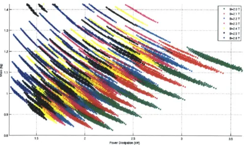
1-2 Power dissipation versus mass trade off curve for doubly-wound motor near 2400 W. Each data point represents the performance of one motor design . . . . 16

1-3 Power dissipation versus mass trade-off curve for permanent-magnet motor at 40 Nm over a wide power range. Each data point represents the performance of one motor design. . . . . 16

1-4 Power dissipation versus mass trade-off curve for permanent magnet motor near 2400 W at 40 Nm. This figure is an expansion of Figure 1-3. ... ... ... 17

1-5 Power dissipation versus mass trade-off curve for permanent magnet motor near 2400 W at 50 Nm. . . . . 17

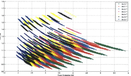
1-6 Power dissipation versus mass trade-off curve for permanent-magnet motor at 50 Nm over a wide power range. Each data point represents the performance of one motor design. . . . . 18

1-7 Fundamental motor layout . . . . 18

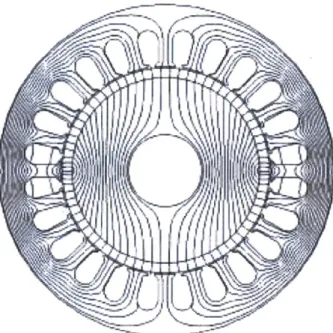
1-8 Example of motor flux lines . . . . 19

1-9 Design approach flow chart. . . . . 21

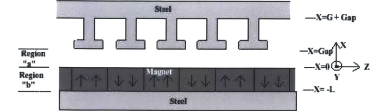
2-1 Magnet only model for the designed motor. . . . . 24

2-2 Current only model for the designed motor. . . . . 29

2-3 Complete model for the designed motor. . . . . 31

2-5 Chart of all designed dimensions. . . . .

3-1 Final motor design front view illustrated with MATLAB. . . . . 3-2 Final motor design side view illustrated with MATLAB...

3-3 Hyperco 50 B-H curve used as a design input. . . . . 3-4 Magnetic field lines for designed motor depicted with COMSOL. 3-5 Motor torque profile data collected from COMSOL. . . . .

3-6 Cogging torque derived through FEA . . . .

4-1 4-2 4-3 4-4 4-5 4-6 4-7 4-8 4-9 4-10

Complete motor 2D image. . . . . Complete motor of 3D image... Drawing of designed stator . . . . Drawing of stator zoomed in. . . . . . Phase A beginnging the wiring process Phase B beginnging the wiring process Phase C beginnging the wiring process Winding Process . . . . Magnet and Rotor . . . .

Complete Motor . . . . 37 40 41 42 46 46 47 . . . . 50 . . . . 51 . . . . 52 . . . . 53 . . . . 56 . . . . 56 . . . . 56 . . . . 57 . . . . 58 . . . . 59

5-1 Moment arm addition made to the motor . . . . 5-2 Measured back EMF from experiments . . . . 5-3 Three phase torque from Back EMF measurements currents of 60 A. . . . . 5-4 Three phase torque from FEA analysis . . . . 5-5 Cogging torque derived through FEA . . . . 5-6 Cogging torque derived through measured values . . 5-7 Voltage change over time calculated . . . . 5-8 Simplified thermal rc circuit for the motor... 5-9 Temperature over time measured and calculated B-i COMSOL Screen Shot . . . . 62 65

. . . .

Chapter 1

Introduction

In the process of creating, potentially, the fastest quadruped robot, a need for a low-mass motor presented itself. To fulfill this need a new motor design was sought that would decrease the mass and maintain the torque output, when compared to the robot's current motor. This thesis focuses on the design, fabrication, and testing of a light-weight motor that both decreases the mass and nearly doubles the torque production. The following introduces the robot the motor is designed for and the approach taken to produce a design that exceeds the goals of the project.

1.1

Project Description

Currently, the Biomimetic Robotics Lab at MIT is working to build the first quadruped robot that can move at a pace equivalent to a running human. Application for this robot is reflected in the Department of Defense's desire to use robotics to carry pay-loads into potentially dangerous and uneven terrain. The use of robots will poten-tially save lives and time, and provide reconnaissance in possibly unfriendly areas. The Biomimetic Robotics Lab attempts to address this desire with a cheetah-inspired robot named The MIT Cheetah Robot. While previous robots have tried to solve the problem of quadruped robotic design using hydraulics [1], the MIT Cheetah Robot will rely on electromagnetic propulsion principles. One component of this robot is a high-torque low-mass motor that will allow for high agility and speed. The total

Figure 1-1: MIT Cheetah Robot conceptual design.

mass of the robot is expected to be 33 kg. The electric actuators for the robot cur-rently weigh 16 kg, consuming almost half of the total mass allowance for the robot. The large consumption of mass by the motors prompted the need for an efficient high-torque lower-mass motor design.

This project attempts to design, fabricate and test a low-mass brushless motor that will produce the same torque and power dissipation while drastically reducing the mass consumption. This, in theory, will allow the robot to reach higher accelerations and speeds, and/or allow for more mass consumption to be spent in other features of the robot such as cooling. This will also permit a higher payload mass. The motor design will be more effective by being customized to meet all the needs the group has. A potential financial savings may occur due to in-house design, fabrication, and implementation. Once the motor design is tested for performance, it will be incorporated into the shoulders and hips of the robot.

1.2

Robot Description

Figure 1-1 shows conceptually what the MIT Cheetah Robot will look like and where the newly designed motors will be utilized. As seen in Figure 1-1, the densest areas of the robot are where the motors will be utilized, namely at the hips and shoulders. The motor design achieved through this project achieved a mass that is 23% lower

Motor Comparison

Description Old Motor New Motor

Mass 1.3 kg 1 kg

Maximum Torque 23 Nm 60 Nm

Power Dissipation at Maximum Torque 2400 Watts 2400 Watts

Table 1.1: Critical design requirements and performance characteristics as per finite element analysis.

than the current motor being used. While the maximum torque of the current motor is 23 Nm, the new design has a maximum torque of 60 Nm, per finite element analysis (FEA) . _{One of the design specifications is a maximum 2400 W power dissipation at}

24 Nm, which is at a 20% duty rating as needed by the robot. A summary of critical design requirements is given in Table 1.1, as well as predicted designed performance characteristics.

1.3

Application

This design also has applications in other high speed robotics, scooters and electric vehicles due to the high-torque low-mass combination. The high torque production of the motor provides the ability to reach higher speeds and accelerations in all applica-tions. Within hybrid electric vehicles, high torque production at low speeds from an electric motor is necessary to complete the torque-speed characteristic needed to meet the traction requirements. The use of an electric motor also cuts down on pollution and noise [2]. The low mass design is especially useful in scooters and electric vehicle applications where frames are kept to minimal weight in order to improve efficiency.

1.4

First-Pass Comparison

In the process of understanding the fundamental properties and principles of syn-chronous machines, an evaluation of machine configurations is conducted. Particu-larly, the qualities of doubly-wound and permanent-magnet synchronous motors are

evaluated. The design that out performs its competitor is chosen to proceed to sub-sequent design steps.

In a doubly-wound motor, the field windings on the stator and rotor are used to produce a magnetic flux. The flux from one winding interacts with the current in the other to produce a torque [3]. The use of current windings on both the stator and rotor produce double the power dissipation over its permanent-magnet competitor which replaces one of the windings with a magnet array. Although the power dissipation is increased, the maximum current is not limited by magnet demagnetization current limits. Therefore, flux and torque outputs are only limited by heat constraints. The mass of a doubly-wound motor can also be less due to the higher density of magnet versus copper. Consequently, both motors should be considered.

A permanent-magnet motor replaces the field windings around the rotor with permanent-magnets. With half the field windings, the total power dissipation is cut by half compared to that of the doubly-wound motor. Depending on the strength of the motor, a higher flux can also be created with less heat. The presence of magnets forces introduces concerns over demagnetizing currents. Unlike in the doubly-wound motor, the current cannot be increased indefinitely. After the demagnetizing current is reached, the magnet will no longer be usable. The density of the magnet chosen can also resort in a higher mass-torque relationship.

In an attempt to choose between the doubly-wound and permanent-magnet syn-chronous motors, a first-pass comparative analysis is carried out along the lines of what is described in more detail in Chapters 2-4 for the permanent-magnet motor. The results are summarized here. The result of this comparison is that the permanent-magnet motor is expected to out perform the doubly-wound motor. Consequently, only the permanent-magnet motor is described in detail in subsequent chapters.

Along with the general differences mentioned previously, the permanent-magnet motor out performs the doubly-wound motor in several other ways. The excitation from the permanent magnets is lossless allowing the motor to be more efficient due to the decrease in excitation. The lossless property of the magnet also allows for a higher pole count design. With more poles, the total flux can be distributed in smaller

amounts, allowing for a decrease in back iron thickness [3]. Decreasing the back iron thickness consequently decreases the total mass of the motor. While it is possible to increase the number of poles in any brushless motor design, this same change will result in an increase in power dissipation with a doubly-wound design. When attempting to maintain a constant flux value, increasing the number of poles increases excitation current which increases loss. This trade off doubles in the doubly-wound motor.

To verify the advantages of the permanent-magnet motor over a doubly-wound motor, power dissipation-versus-mass curves, at a torque of 24 Nm, were constructed using the analysis presented in subsequent chapters. Power dissipation versus motor mass is observed because these are the two primary performance factors once the torque is fixed at 24 Nm. These curves demonstrated the possible torque-mass com-bination that could be achieved from each design with varying design parameters. Figure 1-2 shows the possible trend for doubly-wound motors with a power dissipa-tion close to the 2400 W requirement. When the same analysis was performed on the permanent-magnet motor the power dissipation was far lower than the requirement, therefore the torque was increased to 40 Nm. Figure 1-3 shows the total trend for all possible permanent-magnet designs while Figure 1-4 shows all possible designs near the power dissipation limit. When the torque is increased to 50 Nm, as in Figure 1-5, a design with an even higher torque is achieved with still a considerable decrease in mass. The lowest mass design at 2400 W shown in Figure 1-6 was chosen as the design to fabricate. From these curves, it is evident that a lower mass design with a higher torque can be achieved with a permanent-magnet design. Consequently, only this design is considered in subsequent chapters.

1.5

Approach

The design process followed in this thesis begins with research in the fundamental behavior of a different motor configurations. From various figures, such as Figure 1-7 [3], the fundamental dimensions and characteristics can be learned, thereby, helping to

S . *4 **B=32.0 T * * B=I2. T 1 5 - - - B-= T *5 + *B-2.25 T .4.44 B=L3aST 13

- *-**

*

-~4

111111

~

Figure 1-2: Power dissipation near 2400 W. Each data point

versus mass trade off curve for doubly-wound motor represents the performance of one motor design.

1.5 2 2.5 3 3.5

Powr DIsSIpaon QKW

Figure 1-3: Power dissipation versus mass trade-off curve for permanent-magnet mo-tor at 40 Nm over a wide power range. Each data point represents the performance of one motor design.

... .. .. o* 8-20 T + .

et

Power DIss aton (kW)

Figure 1-4: Power dissipation versus mass trade-off curve for permanent magnet motor near 2400 W at 40 Nm. This figure is an expansion of Figure 1-3.

1.8 -- - - - + - - - -B-82.0 T * B-21 T * B-23 T 1.6 - - - 13k-2.3-2A T 1.5 --- B-266 1.1 -. - - .. . . -.. 1. 2 25 3 3.5 4 4.5 6 65 a Power Disspalon (W

Figure 1-5: Power dissipation versus mass trade-off curve for permanent magnet motor near 2400 W at 50 Nm.

. .

. .. .- 0

-~~~ep *:i#~# .: .O- ,#5~~t

-~~ **-2,3T & .... ... . . ... . . ....I! ~ . . 8- .4 1. 10. 1A 12 12 0-.9 0.0 0.7 0.8 26 2.7 2.8 2.9 3

Figure 1-6: Power dissipation versus mass trade-off curve for permanent-magnet mo-tor at 50 Nm over a wide power range. Each data point represents the performance of one motor design.

-~r. - \ £torb s~kka.

aroof Polo\

qROW He.' S.wre

Figure 1-7: Fundamental motor layout.

define necessary design parameters in the geometry of a motor. Preliminary research also consists of understanding the impact and geometry of flux lines as shown in Figure 1-8 [4]. The understanding gained is used to design configurations that effectively produce maximum motor torque outputs with minimum cogging torque outputs.

2 21 22 22 2A 2-5

Power Dinipaon (

-046A

--.-.-- ...-.- -.-- -.- ..-- .

Figure 1-8: Example of motor flux lines

In order to out perform the current robot, several designs are considered. Each motor design is evaluated to find a design that has the best torque-to-mass ratio. After a design is chosen, all possible dimensions of the design are evaluated to find the best performance for the design. A higher flux steel is also used for all designs so that less steel is needed to carry the same amount of flux. This drops the mass of the total motor. With the cut in mass, the magnet thickness can be increased to produce more torque.

Figure 1-9 summarizes the design process used to formulate a final design. Using Maxwell equations and the desired layout of the motor, several defining modeling equations are formulated. These modeling equations define steel thickness, magnet thickness, number of pole pairs, axial length, slot fraction, packing factor and radial distances. For each of these dimensions, arrays of possible values are constructed. Both the equations and the arrays are fed into a MATLAB script that calculates the necessary output parameters for the correlating combination of input parameters. Output parameters consist of the motor mass, motor torque and power dissipation. The MATLAB script then produces all of the possible designs for every combinations of the design parameters. These designs are filtered by the desired design

specifica-tions so that only the designs that meet all specificaspecifica-tions are left. The specificaspecifica-tions include a power dissipation requirement and the desire for minimal mass. These designs are checked for feasibility and any design that cannot be fabricated due to limitations in achievable steel thickness or widths are removed. From the remaining designs, the design with the lowest mass is manually selected. This design meets all of the design specifications and is governed by the fundamental electromagnetic equations. For a final logic check, the design is passed through finite-element analysis to verify that it behaves as expected and all previous calculated output values are equivalent. The final design is, finally, built and tested.

To make the in-house fabrication possible, several materials are purchased from specialty vendors. Steel laminations are purchased from a manufacturer that cuts, anneals and glues them into a stacked stator and rotor. These laminations are used for the rotor and steel fabrications. Specifically shaped neodymium boron magnets are purchased in shapes that match the geometry of the design and are glued to the rotor. Copper wire is wound around the stator as a source of current and magnetic flux. Bearings are provided by the Biomimetic lab to encase the complete design. Slot liners are used in the stator to prevent scraping of wire when being sewn in. To test the accuracy of the design, motor torque and cogging torque measurements are taken on the now fabricated motor.

1.6

Challenges

From the discussion of torque-mass pairs presented earlier, it can be understood that one of the major challenges of an effective design is finding the right balance between these two parameters. Torque is directly related to the amount of flux present. In a permanent-magnet motor design, the only two contributers of flux are the armature current and the magnet. The armature current is limited by the demagnetizing current and heating restrictions. Therefore, the most efficient way to increase the flux, and subsequently the torque, is to increase the strength or size of the magnet. Magnet strength is limited by the cost of current technology and the

Defining input equations

and output parameters are

combined to find all

possible combination of

motor designs

Optmzto

Final

design is

passed

through

F

A for

verification

cost of leaving the magnet thickness as the most volatile parameter. Since the magnet has the highest density compared to other materials used in the motor, the magnet thickness directly affects the total mass of the motor. This intricate relationship between torque and mass compels a search for a design that has the most effective partnership of torque and mass. This search is described in the following chapters.

Chapter 2

Formulation

This chapter formulates the motor design equations. These equations are the product of basic electromagnetic principles and the design specifications for the motor. The equations formulated will provide exact values for all of the defining characteristics of the motor. They underlie the design process described in later chapters.

2.1

Simplified Model

To form discrete equations, a simplified model of the motor is used. Based on super-position this model can be broken into two parts. The first part consists of magnetic fields driven by the magnets only; the second consists of magnetic fields driven by the winding currents only. The permeability of the steel is taken to be infinite in both cases to simplify the solutions of Maxwell's equations.

2.2

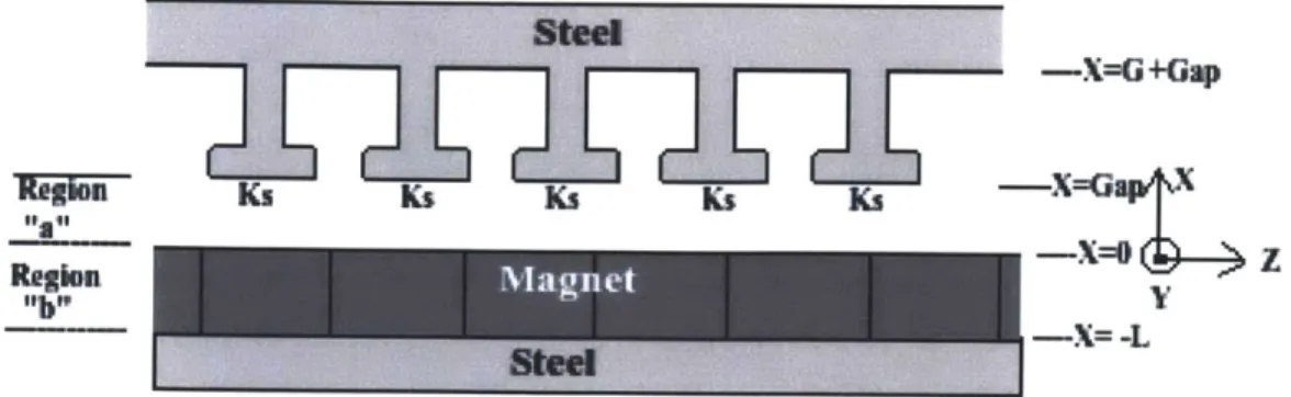
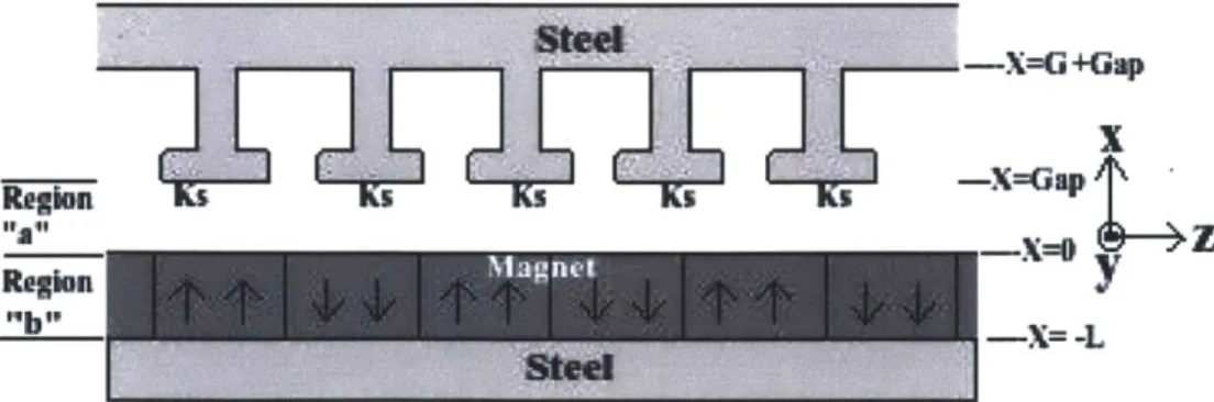
Magnet Model

In this section all calculations are performed using a model where the magnetic fields are driven by the magnets only. The permeability of the steel is simplified to be infinite. Referring to Figure 2-1, the magnets thickness is L and the length across the air gap is Gap. Region "a" consists of the space within the air gap and region "b" consists of the space within the magnets. The result of the following calculations are

-X=G+4- Gap

Regiou _VXa4

_____7 _{-X= 4L}

Figure 2-1: Magnet only model for the designed motor.

expressions of the magnetic fields in Regions "a" and "b" when the magnetics are the driving source. A depiction of this setup can be seen in Figure 2-1.

Analyzing the magnet-only configuration begins with Ampere's Law.

0 0

fH-ds=J (2.1)

Since the magnet-only configuration contains no current, the second integral term goes to zero. The third integral term also goes to zero due to the absence of time variations. Therefore Ampere's law reduces to:

H - s = 0 (2.2)

Utilizing boundary conditions from Ampere's Law, the simplicity of the permeability of the steel, the tangential components of the magnetic field strength at the interfaces x=-L and x=Gap must got to zero. The tangential component is denoted by the symbol ||. The magnetic field strength solved in a region is denoted with a subscript of the direction and the region. For example, HyloX=G is the tangential component of the magnetic field strength in region "a" at the position x=G. Therefore,

HilsIx=_L = 0 H a Ix=Gap = 0 (2.3)

(2.4)

Hia x=O = HIlbJoxb=O =

Hxo

From Gauss' Law, the closed surface integrals of magnetic flux in both regions "a" and "b" must also vanish. The magnetic flux derived below is used later in this chapter to form a complete expression for the magnetic flux. Here,

B -da = 0

(2.8)

from which it follows that

B1a = Bib Ix=o (2.9)

(2.10) (2.11)

Bia = po -Hai Bib = p1o(Hbi + M)

Here, the symbol "I" denotes a perpendicular component. M is the magnet magne-tization in the x direction which naturally resembles a square wave, as seen in Figure 2-1. The square wave of the magnetization is approximated by taking the first term where

of the Fourier series expansion. This approximation

M = 4M cos kz (2.12) 7r

is used to find the magnetic flux in the "a" and "b" regions.

Knowing the general form of the magnetic field, the magnetic scaler potential can be derived. The potential must be formulated from a combination of cos, sin, cosh, and sinh such that H=-VV and

v

'V

a

i/cos(kz) sinh[k(x - Gap)] (

sinh(-kGap)

$

O cos(kz) sinh[k(x + L)] ( sinh(kL)

From these magnetic potentials we can formulate the magnetic field as

-k'padcos(kz) cosh[k(x - Gap)]

Hxa = sinh(-kGap)

(2.15)

Hza =p -k1adsin(kz) sinh[k(x - Gap)]

(2.16)

kobd cos(kz) cosh[k(x + L)] (217)

sinh(kL)

kVpbd sin(kz) sinh[k(x + L)] ( sinh(kL)

These magnetic fields naturally satisfy the boundary conditions at x=Gap and x=L. Utilizing the previously derived boundary conditions, the magnetic field can be

for-mulated for the boundary at x=0 according to

Hzalx= -

-kpad sin(kz) sinh(-kGap)

(2.19)

sinh(-kGap) = kp)adsin(kz)

Hzblxo

(2.20)

sinh(kL) = kV~/dsin(kz)

From Equation 2.6 both parts of Equations 2.19 and 2.20 equal. Therefore,

k'ad sin(kz) = k'z/ sin(kz) (2.21)

Vyad = 'bd =

so that

Hxalx-j - -k$ cos(kz) cosh(-kGap) (2.22)

sin(-kGap)

Hxbl x=O- -kip cos(kz) cosh(kL)

(2.23)

sinh(kL)

Now that the magnetic field has been derived the magnetic flux can be formulated from Equations 2.10 and 2.11. This yields

Bx = Yo- ko cos( kGap) cosh(kz) (2.24) sinh( -kGap)

-kt cos(kz) cosh(kL) 4 90V sin(kL)

+

-kpcosh(-kGap)

(2.25)

Hyperbolic long-wave functions (kGap<<1) approach asymptotes; a sinh function approaches the argument at which it is evaluated, while the cosh function approaches

1. After long wave approximation ib can be further simplified to Mo4 -k___ (2.26) -kGap ±e~L Mo 4 G~ap L GapLMo ' Gap + L

Utilizing Equations 2.7 and 2.10 as well as the equation for the magnetic flux in the "a" region completes the magnetic flux calculation for the magnet-only configuration. This result is

B = poHxajx=0 (2.27) pokGapLM04 cos(kz) cosh[(k(x - Gap)]

ir(Gap

+

(2.28)

After long wave approximation,

pokGapLMoA cosh(kz)

Bx = 7 (2.29)

(Gap + L)(-kGap) _ pOLM₀4 cos(kz)

,r(Gap+ L)

in both regions "a" and "b".

2.3

Current Model

The current-only model is analyzed in a similar manner as the magnet-only model. By evaluating Ampere's Law at the boundaries, the magnetic scalar potential, @', can be chosen to match the magnetic field. Once V is derived, the magnetic field and magnetic flux can be easily formulated. In this model the windings are approximated as a surface current at x=Gap. Ks in Figure 2-2 denotes this surface current. It is a sinusoidal approximation for the three phase currents in the slots in the stator. The

-X=G4Gap

-X=0

z RegimnMge_I"

-X= -L

Figure 2-2: Current only model for the designed motor.

model, similar to the magnet-only model, is divided into two regions, and values Gap and L again represents the air gap and magnet lengths respectively. In the current only model, the important boundary conditions are

HilbI~x=-L = 0 (2.30)

HilaI\x=Gap =

k,

(2.32)

Since the magnets are replaced by free space in the current-only model, the magnetic potential need only be a single function 0 that is valid in both regions "a" and "b". Thus,

p,

sinh[k(Gap+ L)]

(2.34)

from which it follows that

H= -kp,' sin(kz) cosh[k(x + L)] (2.35)

sinh[k(Gap + L)]

Hz = kp. cos(kz) sinh[k(x + L)] (2.36)

Hzlx=Gap -

-k@, cos(kz) sinh[k(Gap +

(237)

sin[k(Gap

+

= -- kV, cos(kz)

Knowing that the magnetic field at the boundary of x=Gap must equal the surface current (K), an exact solution for it can be formulated as

HzIx=Gap = -kp, cos(kz) = K, cos(kz) (2.38)

k, = -k@, (2.39)

At this point, a complete equation can be formulated. This equation is then simplified using long wave approximation and used to formulate the magnetic flux and field as

Hx = k. sin(kz) cosh[k(x + L)] (2.40) sinh[kGap + L)] k, sin(kz) k(Gap + L) Bz = 1ok, sin(kz) (2.41) k(Gap+ L)

2.4

Combining models

Due to linearity of both models, superposition applies, and both configurations can be combined to form the actual configuration used for the motor design. The magnetic flux from Equation 2.29 and Equation 2.41 can be combined to derive the total magnetic flux in the motor according to

pIlok, sin(kz) 1 0LM04 cos(kz) (

-X=-L

Figure 2-3: Complete model for the designed motor.

Using the surface current applied at the stator, the sheer stress acting on the stator can be formulated as using the cross product of the surface current and the total magnetic flux. This results is

K =

k,

Area =kxB(.4

po~k! costkz) sin(kz) ±pok8LMo4 cos2 (kz) _

k(Gap±+L)

+L

)

piokn sin(2kz) pokLMi

cos

₍

_{kz )}

= -X+ )z

2k(Gap+±L)

(Gap+±L)

The average stress can be formulated by integrating the over a single period. This average stress can be used to calculate the torque by taking the cross product of

the motor radius and the average stress then multiplying by the complete area. The

result is

1 Fw Force

Average Stress

2

1 1

dzdw

(2.45)

k

w2kr o o k(Gap + L) Gap+ L

_ 2pzokLMo

The torque (r) can be defined using the using the previous stress force from Equation 2.45, the moment arm R and the area A according to

7 = (R x F)A (2.46)

R2kL _2rRW

r(Gap + L)

R24 poksLMow

(Gap + L)

The torque found in Equation 2.46 is the basic design equation for the motor. This equation has several limitations. As seen in Equation 2.12 only the first term of the Fourier series expansion is used to find the magnetic flux. This equation for torque does not take into account saturation and thermal limits. Cogging torque also is not considered since the stator and rotor surfaces were assumed to be smooth.

2.5

Design Parameters

Several of the motor parameters can be deduced from the Maxwell's equations above, while others are defined by the given motor parameters. Using all of these equations a MATLAB script is written to design the motor. The script will take in several inputs, some of which vary over a range of values, and will output five parameters. The inputs include the magnetic flux in the steel, the slot fraction, the outer radius of 0.0603 m, the stack width, number of poles, gap thickness, the stack tooth length and the torque. From these parameters, the script will determine the steel thickness, the magnet thickness, the surface current, mass and power dissipation. The equations defining each of these parameters is defined in this section.

Knowing that all of the flux that passes through the stator teeth must, also pass through the back iron, an expression for T, the steel thickness, can be formulated so

that the back iron carries the same flux density as the stator teeth. This results is 27rR 2 (1 -6)Hteei = -THteel (2.47) 6P 3 piR 3

T - pi(1 - 6)-3

where 6 is defined as the slot fraction, or the ratio of empty space to steel for each pair of spacing and rotor teeth. The parameter is limited to 0.2-0.8 to make fabrication possible. Finally, Bmag and Bap are related to Bteel by

Bgap = Bmag (2.48)

= (1 - 6)Bsteel

(2.49)

Using Ampere's law around a closed path, an equation for the magnet thickness

can be made. Each section of the motor is broken into sections and the magnetic field strength around the motor must equal zero. The subscripts in Equation 2.50 signifies the region the magnetic field belongs to.

2_{HgapGap + 2HsteeiG + 2Hsteet 27rR + HmaL = 0 (2.50)}

2P

L

+ HsteeiG + Hsteei

Hmag

R is defined as the radius from the motor center to the midpoint of the gap between

the stator and the rotor. This value will be varied to find the best combination, along with the stator width (W) and the number of pole pairs (P). G is defined as the length of the stator tooth. The gap (Gap) is a fixed dimension of 400 pm.

Equation 2.51 is used to find L from an assumed set of flux linkages. The initial flux linkage is Bsteel which sets Hteei while Hmag and Hgap follow from Equation 2.48. Next torque and L are used to determine k, from

k, = 4 TM W(2.52)

assuming -r is 24 Nm. Finally power dissipation, PD, is determined from k, as dis-cussed below.

After each of the output parameters are defined, the mass, M, can be calculated using the density of each of the materials.

Mass = [,r(R + G + T)2 - ,r(R + G)2]Wpteel (2.53) +[,r(R + L)2 _{- ,r(R - L - T)}2_|Wpsteel +[,r 2 - ,r(R - L)2 WPNdBFe +[,r(R + G)2 _{- r R}2_{] (1 _ 6)Wpsteel} +[wr(R + G)2 _{- ,rR} 2|6Wpo per

where W, denotes W+z to account for the space taken up by the end turns. To form an equation for power dissipation, the total current is found from the surface current and the resistance is found from the standard equation

4

the packing factor which affects the effective area. The length of the wire, 1, can be calculated from the arc length around three teeth and the width of the motor. This path is repeated P times, where P is the number of pole pairs. The area is defined as the area of the spacing of one slot fraction. Once a number of turns is decided, this value is multiplied by the resistivity value to find the total resistance. Considering each pole, the wire arcs with a diameter of * then travels the thickness motor as seen in Figure 2-4. Thus, the length 1 is given by

1= _2P2P +W)2P (2.54)

=,r2R +W2P

The area, A, can be calculated by determining the area of one slot.

2irR

A=6 G (2.55)

2P3

6,rRG

pPR*

wire

Figure 2-4: Resistance Calulation

Using Equation 2.54 and Equation 2.55, a equation for total resistance can be formulated according to Total Resistance = a

p(wr

_{R +}

_W2P)

pf 6rWRG

Using the length of one slot and the surface current (k.) the total current (I) can be determined. Using the current and the resistance in Equation 2.56 the power

dissipation PD is derived. Ig =k (2.57) 3P PD = 2-RI2 (2.58) S33pP 2[2W + ] k,1rR 2 2 GirR6pf 3P _

w+i2R]

From all the equations derived previously Equations 2.47 and 2.50 are used in Appendix A to define key parameters of the motor and ensure that saturation is being taken into account. Equations 2.52, 2.53, and 2.57 are used to weed out designs that do not have favorable performance.

2.6

Optimization

The MATLAB script, written to find the best motor design, considers all of the possible combinations of motor parameters from the possible inputs and calculates the five desired output parameters. The exact script can be found in Apendix A. The input parameters include the magnetic field in the core with saturation considered, the slot fraction, outer radius, axial width, the motor torque number of pole pairs, air gap length, length of stator teeth, magnetic strength, packing factor and densities and conductivity of steel and copper. The output parameters include the steel thickness, the magnet thickness, the mass of the motor, the power dissipation and the surface current. The torque is set to 40 Nm. From all of the designs, any design that has a power dissipation that did not fall within a 10% tolerance of 2400 Watts is eliminated. From the remaining designs, the design with the lowest mass is inspected for accuracy. The final design is one that met the power dissipation, has the lowest mass and is the most feasible to fabricate. The code also output five of the defining radii. R5 is defined as the radius from the motor center to the outer edge of the motor. R4 is defined as the radius to the start of the stator back iron. R3 is defined as the radius

R5 stee R4 L Magnet T _steel R3 R2 R1

Figure 2-5: Chart of all designed dimensions.

to the magnet edge. R2 is defined as the distance to the edge of the rotor back iron and RI is defined as the distance to the start of the rotor back iron, as seen in Figure

2-5. Since the project currently uses an off the shelf motor, it is desirable to keep the

same housing or outer radius (R5). Thus, R5 is defined as 0.0635 m. This forced the input parameter R to be defined in terms of R5. Since R5 is the outer radius, it can be defined by all of the radii smaller than it as

R5 = R +

±

+rR(l

) +G

(2.59)

6)

2P

2

R(

R5-G

R5

G

Chapter 3

Design

The design process is the final step before the fabrication process could begin. The design discussed in this chapter is the product of the earlier MATLAB script. Deci-sions were made regarding which materials would be used for each component of the motor and final calculations were made on motor characteristics. The final design is verified with finite element analysis (FEA).

3.1

Materials

The motor stator laminations and the rotor laminations were manufactured from Hiperco 50 steel. This steel has a higher saturation than the steel currently being used by the Cheetah motor. The magnets used for the rotor were Neodymium Boron magnets capable of creating a 1.4 Tesla flux. Copper is used to wire the stator, each phase had 60 feet of wire wound around the motor. 2 mil nomex slot liners were used in between each slot to protect the wire when winding. Plastic spacers were used in between each magnet to provide exact spacing around the rotor.

3.2

Dimensions

Using the equations discussed in Chapter 2, the inputs, which consisted of the mag-netic field in the core with saturation considered, the slot fraction, outer radius, axial

004

-.0 -0.06 004 .02 0 0.02 0.4 0.0 0.08

Figure 3-1: Final motor design front view illustrated with MATLAB.

width, the motor torque, number of pole pairs, air gap length, length of stator teeth, magnetic strength, packing factor and densities and conductivity of steel and copper, were varied to produce several possible designs. The outputs for each design include backiron thickness, the magnet thickness, the mass of the motor, the power dissipa-tion and the surface current. Torque was set to 40 Nm for each design. From all of the possible designs, which are shown in Figure 1-3, one was chosen that had the lowest mass and met the power dissipation requirements. The cooresponding dimensions in Table 3.1 were calculated by the script and used in the final design. Figures 3-1 and

3-2 illustrate these dimensions in a motor drawing produced by the MATLAB script.

These dimensions are used to calculate the motor characteristics, such as peak torque, peak cogging torque, and thermal performance. The predicted performance was then verified with FEA. To determine the flux in the steel with saturation taken into account, measurements were taken from the curve in Figure 3-3 [5]. A vector of flux values and corresponding p values were taken from the Hiperco 50A strip curve in and used in the MATLAB script as the magnetic-field-in-the-core input. These values were also used in FEA analysis to define the steel. This can be seen in Appendix B.

0.00 O.0 -0 404 -08

I

LI

]1

]

-0.F -00 F 0i04 deig -. 0 0s04 0i0l 0.8

Figure 3-2: Final motor design side view illustrated with MATLAB.

Dimensions

Value

Slot Fraction

0.46

R5

0.0635 meters

R4

0.0603 meters

R3

0.0485 meters

R2

0.0417 meters

RI

0.0385 meters

R

0.0486 meters

T (steel thickness) 0.0032 meters

W (axial length)

0.0150 meters

G (winding length 0.0115 meters

L (magnet length) 0.0095 meters

Pole Pairs

13

Air Gap

400 pm

Table 3.1: Motor Dimensions

-Typical D.C. Magnetization Curves-Hiperco 50A Alloy vs. Electrical Iron 24 r I I I I . .

-o

Mmgnstizing Foro (H, Oersteds)

Hiperco 50A strip, .055" (.89 mm) thick,

1600*F

(871 *), 2 hr., dry H,.

Hiperco 50A

bar, 1875*F (1010C),

water quenched

plus 1600*F (871 *), 2 hr., dry H,.

Hiperco 50A bar, 1600*F (871*C), 2 hr., dry H,. Hiperco 50A bar, 1533*F (820*C), 2 hr., dry H,. Electrical Iron bar, 1550*F (843*C), 4 hr., wet H,, FC.

1000

Figure 3-3: Hyperco 50 B-H curve used as a design input.

20 16 12 a 0 4

3.3

Mass and Rotor Inertia Calculations

With the materials defined, Equation 2.53 can be used to calculate the mass of the motor using the motor dimensions and the mass densities of copper, Hiperco 50, and Neodymium Boron. This calculation yields a mass of 1.07kg. Since the rotor is the only moving component, the inertia (I) is calculated on this component only. The inertia is calculated from the rotor mass M,,,t, and the radius to the rotor steel and the radius to the magnet edge.

1

I = Mrotor (rl 2 _{+ r2}2_{) (3.1)}

2 Its value was 0.468x10-3kgm2.

3.4

Resistance and Inductance Calculations

Using Equation 2.56, a value for resistance can be calculated using the values from Table 3.1. This value will be used when determining the number of turns and the current density for simulation purposes.

To calculate the line to neutral flux linkage, Farady's law of induction is used to find a relationship between the driving flux and the resulting flux linkage.

d

f

From Equation 3.2 it is clear that the flux linkage only depends on the current ex-citation in the stator. Using the current-only model described in Section 2.3, an expression for flux can be taken from Equation 2.41. Since this design contains con-centrate winding, Equation 3.2 can be used to calculate the flux linkage, where N is

the number of turns and A is the area that the windings occupy. Thus A = Bds (3.3) =NBA

2,rR

N

oIrWR

Using the flux linkage calculated in Equation 3.3 and comparing it to Equation 3.2, a closed form expression for inductance is formed as

L =

-

_ N2 po7rW R Gap+ L

This inductance has to be added to the slot leakage inductance to determine the total line-to-neutral inductance of the motor. The slot leakage can be calculated using the magnetic flux in each slot which is, in turn, computed from the energy stored in each slot. The calculations below are performed using the geometry depicted in Figure 2-3 to yield J

Ni

1H2

ON

po

N

WG

where x in the above equation signifies the distance parallel to the slot. The expression

R denotes the distance across the slot in the angular direction. By combining

Equations 3.4 and 3.5, an expression for the total inductance is determined to be

N 2 porWR poN 2WG

L =

±

2P

(3.6)

Gap+L 3("r)

3.5

Finite Element Analysis

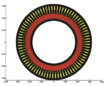
The finite element software COMSOL is used to verify the design. Using the dimen-sions from Table 3.1, a drawing is created for the motor. This drawing is imported into COMSOL, which used the dimensions and the parameters defined in Appendix B to solve Maxwell's equations and create images of the flux lines. One of these images can be seen in Figure 3-4. COMSOL is also used to create a torque-verse-position graph using its ability to calculate shear stress.

From Equation 2.56, we know that the resistance is based on the packing factor. By keeping a constant 2400W Power Dissipation a current corresponding to various packing factors can be calculated due to the varying resistance values. This current can be converted to a current density by dividing by the winding area. This current density is used in the COMSOL simulation. The position of the rotors was varied to create a full motor torque and cogging torque swing which is seen in Figure 3-5 and Figure 3-6. The peak torque value is then used to make a torque-verses-current and packing factor comparison. These values are compared in Chapter 5 to the experimental measurements reported in Chapter 5.

All FEA analysis was done with a 50% packing factor, since this was thought to

be easily achievable. Using the packing factor and the fixed power dissipation it was determined that eighteen turns were appropiate. From FEA and the MATLAB script output results, the designed motor is expected to weigh 23% less than the current motor and produce 2.3 times more torque at 60 Amps and 50% packing factor. Since this design met the desired goals, the fabrication process began.

Surface: Magnetic field norm (A/m) Contour: Magnetic vector potential (Wb/m) S11 A 2.524x106 x106 2.5 0.04 2 0.02 1.5 0 1 -0.02 0.5 -0.04 y 30.54 -0.06 -0.04 -0.02 0 0.02 0.04 0.06

Figure 3-4: Magnetic field lines for designed motor depicted with COMSOL.

Motor Torque Vs Position

80 60 40 -20 0 213 46 9i2 11.51381. 118420. 26.327.62$.931.2 536.839.141.4437 46 4A 65 -20 --40 --60 . . . .. . -80 Angle (degrees)

Cogging Torque vs Angle

- Cogging Torque

-0.03

-Angle (degrees)

Figure 3-6: Cogging torque derived through FEA

0.03 0.02 0.01 z 0 F- 0.00 0.00 -0.01 -0.02

Chapter 4

Fabrication

This chapter focuses on the fabrication of the motor. The first step in the fabrica-tion process, once the dimensions for the motor design were finalized, was to select vendors to produce the magnet segments and laminations for the stator and rotor. Additionally, a wire vendor was chosen. After receiving the magnets, laminations, and wire, the motor was constructed as described in this chapter.

4.1

Hardware

Polaris Laser Laminations (http://www.polarislaserlaminations.com) was chosen to provide the laminations for both the stator and rotor. The company was also able to stack and anneal the laminations. K&J Magnetics (http://www.kjmagnetics.com/) was chosen to provide the magnet segments. They were able to produce magnet segments that were the exact arc segment as designed. EIS (http://www.eis-inc.com/) was chosen to provide the wire for winding the stator phases.

4.1.1

Laminations

Steel laminations for the rotor and stator were made from 14 mil Hyperco 50 steel. The stator has an outer diameter of 5 inches and the rotor is a 3.28-inch outer diam-eter ring. Both laminations were made from 0.59-inch high stacks and bonded with

Figure 4-1: Complete motor 2D image.

Rembrandtin EB-548 coating.

Several design drawings were constructed using the softwares SolidWorks and AutoCad. These drawings were used for FEA analysis and sent to the previously mentioned steel and magnet vendors. Figure 4-1 shows a drawing for the complete motor. This 2D drawing can be turned into a 3D representation as seen in Figure 4-2. More specific drawings of the rotor and stator were sent to the laminations manufacture so the design is as exact as possible. Figure 4-3 and Figure 4-4 shows the details of the stator including the key ways that were spaced 120 degrees apart. These drawings helped provide a more realistic visual of what the motor would look like, whether the design was feasible, and if the aspect ratios were acceptable.

4.1.2

Magnets

Twenty-six arc-magnet segments with a 13.56 degree arc were used to form a ring-array of magnets that was attached to the rotor. Thirteen of the magnets were north on the outside face and thirteen were south on the outside face. The outer and inner radius for each magnet is 41.7mm and 15mm, respectively. The arc length was decreased by 2% to allow for manufacturer error. The magnets were grade N42 and are coated with Nickel (Ni-Cu-Ni) to prevent oxidation.

4.1.3

Wire

To wire the motor, 28 gauge copper wire was used. This gauge was chosen because it slid easily between slots making it more feasible to wire by hand. A bundle of eight wires was used for each turn. The highest packing factor was attempted by wiring as many turns as possible. FEA calculations were performed using a packing factor of 50%, for power calculations to set current density, and eighteen turns. During hand wiring only fourteen turns could be achieved, and this reduced the packing factor to approximately 35%.

To protect the wire from being scratched by the laminations and possibly causing a short, a 2 mil slot liner was used in each slot. The liner was cut to shape and placed in the slot before the wire was inserted. After the wiring process was completed the liner was cut down so that it did not protrude into the gap.

4.2

Procedure

Once all of the components were received, motor assembly could begin. The assembly process included wiring the stator, gluing and aligning the magnets to the rotor, and encasing the stator and rotor so testing could commence. The motor was not potted, though this should be done eventually in order to improve thermal performance.