Climatologies of streamer events derived from a transport model and a coupled chemistry-climate model

HAL Id: hal-00301007

https://hal.archives-ouvertes.fr/hal-00301007

HAL is a multi-disciplinary open access

archive for the deposit and dissemination of sci-entific research documents, whether they are pub-lished or not. The documents may come from teaching and research institutions in France or abroad, or from public or private research centers.

L’archive ouverte pluridisciplinaire HAL, est destinée au dépôt et à la diffusion de documents scientifiques de niveau recherche, publiés ou non, émanant des établissements d’enseignement et de recherche français ou étrangers, des laboratoires publics ou privés.

Climatologies of streamer events derived from a

transport model and a coupled chemistry-climate model

V. Eyring, M. Dameris, V. Grewe, I. Langbein, W. Kouker

To cite this version:

V. Eyring, M. Dameris, V. Grewe, I. Langbein, W. Kouker. Climatologies of streamer events derived from a transport model and a coupled chemistry-climate model. Atmospheric Chemistry and Physics Discussions, European Geosciences Union, 2002, 2 (6), pp.2297-2342. �hal-00301007�

ACPD

Full Screen / Esc

Print Version

Interactive Discussion

c

EGU 2002

Atmos. Chem. Phys. Discuss., 2, 2297–2342, 2002 www.atmos-chem-phys.org/acpd/2/2297/

c

European Geosciences Union 2002

Atmospheric Chemistry and Physics Discussions

Climatologies of streamer events derived

from a transport model and a coupled

chemistry-climate model

V. Eyring1, M. Dameris1, V. Grewe1, I. Langbein2, and W. Kouker2

1

DLR Institut f ¨ur Physik der Atmosph ¨are, Oberpfaffenhofen, D-82234 Wessling, Germany

2

Forschungszentrum Karlsruhe, Institut f ¨ur Meteorologie und Klimaforschung, 76344 Eggenstein-Leopoldshafen, Germany

Received: 17 October 2002 – Accepted: 14 November 2002 – Published: 2 December 2002 Correspondence to: V. Eyring (Veronika.Eyring@dlr.de)

ACPD

Full Screen / Esc

Print Version

Interactive Discussion

c

EGU 2002

Abstract

Streamers, i.e. finger-like structures, reach from lower into extra-tropical latitudes. They can be detected in N₂O or O₃ distributions on single lower stratospheric layers in mid-latitudes since they are characterised by high N₂O or low O₃ values compared to undisturbed mid-latitude values. If irreversible mixing occurs, streamer events

sig-5

nificantly contribute to the transfer of tropical air masses to mid-latitudes which is also an exchange of upper tropospheric and stratospheric air. A climatology of streamer events has been established, employing the chemical-transport model KASIMA, which is driven by ECMWF re-analyses (ERA) and operational analyses. For the first time, the seasonal and the geographical distribution of streamer frequencies has been

de-10

termined on the basis of 9 years of observations.

For the current investigation, a meridional gradient criterion has been newly formu-lated and applied to the N₂O distributions calculated with KASIMA. The climatology has been derived by counting all streamer events between 21 and 25 km for the years 1990 to 1998. It has been further used for the validation of a streamer climatology

15

which has been established in the same way employing data of a multi-year simula-tion with the coupled chemistry-climate model ECHAM4.L39(DLR)/CHEM (E39/C). It turned out that both climatologies are qualitatively in fair agreement, in particular in the northern hemisphere, where much higher streamer frequencies are found in win-ter than in summer. In the southern hemisphere, KASIMA analyses indicate strongest

20

streamer activity in September. E39/C streamer frequencies clearly offers an offset from June to October, pointing to model deficiencies with respect to tropospheric dy-namics. KASIMA and E39/C results fairly agree from November to May. Some of the findings give strong indications that the streamer events found in the altitude region between 21 and 25 km are mainly forced from the troposphere and are not directly

re-25

lated to the dynamics of the stratosphere, in particular not to the dynamics of the polar vortex.

atmo-ACPD

Full Screen / Esc

Print Version

Interactive Discussion

c

EGU 2002

spheric conditions, have been employed to answer the question how climate change would alter streamer frequencies. It is shown that the seasonal cycle does not change but that significant changes occur in months of minimum and maximum streamer fre-quencies. This could have an impact on mid-latitude distribution of chemical tracers and compounds.

5

The influence of streamers on the mid-latitude ozone budget has been assessed by applying a special E39/C model configuration. The streamer transport of low ozone is simply inhibited by filling up its ozone content according to the surrounding air masses. It shows that the importance of streamers for the ozone budget strongly decreases with altitude. At 15 km streamers lead to a decrease of ozone by 80%, whereas around

10

25 km it is only 1 to 5% and at mid-latitude tropopause, ozone decreases by 30% (summer) to 50% (winter).

1. Introduction

The stratospheric ozone distribution is influenced not only by in-situ chemistry but also by a broad variety of different dynamic processes, for example tropospheric

dynam-15

ics (e.g.Reed,1950;Dameris et al.,1995), stratosphere-troposphere exchange (e.g.

Holton et al.,1995;Grewe and Dameris,1996;Kowol-Santen et al.,2000), or merid-ional transport in the stratosphere (e.g.Salby and Callagham, 1993; Waugh, 1997). Observations of chemical tracers like N₂O and HNO₃by the CRISTA instrument (O

ffer-mann et al.,1999) or from the UARS satellite (Randel et al.,1993) indicated a strong

20

latitudinal gradient in these trace species, which confirmed the existence of a sub-tropical transport barrier (Plumb,1996). Therefore, (quasi-) horizontal mass exchange between the tropics and mid-latitudes is restricted. Those structures are superimposed with tongues of tropical air (stretching from tropical latitudes to the extra-tropics), which transport tropical air masses into the mid-latitudes. Satellite-based observations of

25

chemical compounds and analyses of meteorological quantities (e.g. Ertel’s potential vorticity) indicate that the remaining transport occurs in form of pronounced finger-like

ACPD

Full Screen / Esc

Print Version

Interactive Discussion

c

EGU 2002

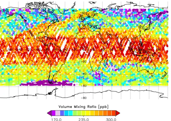
structures, so-called streamers, which frequently appear over the Atlantic Ocean. For example, large areas characterised by low ozone and HNO₃ or high N₂O mixing ra-tios are advected (quasi-) horizontally towards mid-latitudes and are partly irreversibly mixed with surrounding air masses. An example of a CRISTA-1 measurement of N₂O (Version 5) at 30 hPa on November 6, 1994 is shown in Fig.1(Offermann et al.,1999).

5

It is still an open question how streamers are related to large-scale dynamics, i.e. the variability of the stratospheric polar vortex, which is directly connected to the activity of (quasi-stationary) planetary waves. There are hints that the frequency of occurrence as well as the intensity (spatial size) of streamers might be linked to enhanced wave activity (e.g.Waugh,1993). Rossby wave breaking events are capable of eroding the

10

polar vortex, which can cause irreversible mixing. Streamers are often linked to strong vertical and horizontal advection processes. This can cause considerable horizontal gradients, e.g. in ozone concentration, and therefore, parts of the smaller scale ozone variability is due to streamer events. Streamers have been identified at all altitudes between the tropopause and the middle stratosphere (e.g.Waugh,1996;Orsolini and 15

Grant,2000;Waugh and Polvani,2000).

As mentioned above, a considerable number of papers have been published which deal with individual streamer events (e.g.Offermann et al.,1999;Kouker et al.,1999a) or discuss streamer events during shorter (seasonal) episodes (e.g.Chen et al.,1994). A reliable streamer climatology, which requires long-term data series, is currently not

20

available. The seasonal and geographical variations have been determined only on data records of at most 3 years (e.g. Waugh,1996;Orsolini and Grant, 2000) which are different in detail.

In the current paper a numerical method has newly been developed to detect and to count streamers. It focuses on streamers that are mainly caused by horizontal

ad-25

vection and lead to substantial meridional displacements. This method is described in Sect. 2.1. For the first time a 9-year data record has been used to determine a streamer frequency climatology. It is based on calculations of the chemical transport model KASIMA (Sect. 2.2) which uses ECMWF re-analyses (ERA) and operational

ACPD

Full Screen / Esc

Print Version

Interactive Discussion

c

EGU 2002

analyses. In Sect.3, the streamer climatology obtained from KASIMA is presented and discussed. In addition, a respective streamer climatology has been derived from the coupled chemistry-climate model ECHAM4.L39(DLR)/CHEM (hereafter E39/C), which uses the same counting algorithm. The results gained from E39/C have been com-pared to KASIMA. This inter-comparison aims to check the abilities and deficiencies of

5

E39/C with respect to the temporal and spatial distribution of streamers.

Most of the currently available models, in particular chemical-transport models (CTMs) and chemistry-climate models (CCMs) underestimate the observed ozone trend in northern hemisphere mid-latitudes during the last two decades. Certainly, no definite conclusion about the missing processes in the models can be given, although there are

10

several possible explanations (e.g.Becker et al.,1998;Grewe et al.,1998; Solomon

et al., 1998; Steinbrecht et al., 1998). A change of streamer occurrence could also have an impact on mid-latitude ozone changes (trends). Therefore, based on distinct model sensitivity studies with E39/C an analysis of the frequency of streamer events under recent (1960, 1980, 1990) and possible future (2015) atmospheric conditions is

15

carried out (Sect. 4). After examination of E39/C and considering its limitations, it is employed to quantify the importance of streamers to meridional transport of ozone low air to extra-tropical latitudes and for the mid-latitude ozone budget using an artificial E39/C experiment design (Sect.5). A summary and concluding remarks are given in Sect.6.

20

2. Method and model description

In this section, a detailed description of the meridional streamer criterion and a com-parison to other methods is given. Brief summaries of the employed model systems are presented which are used for the current investigations.

ACPD

Full Screen / Esc

Print Version

Interactive Discussion

c

EGU 2002

2.1. Definition of a streamer criterion 2.1.1. The meridional streamer criterion

This study first aims to find an objective criterion to identify streamer events in observed and modelled data sets and to derive a global streamer climatology for all seasons. Use can be made of chemical and dynamical tracers like N₂O, O₃, HNO₃, and (Ertel’s)

5

potential vorticity (EPV), which have strong latitudinal gradients but a pronounced zon-ally symmetric structure under undisturbed atmospheric conditions. The entry of air masses from different latitudes is therefore accompanied by a change of the vertical and the meridional gradient of those tracer fields. Deviations of the gradient can be used to identify regions where horizontal transport processes from the (sub-) tropics to

10

extra-tropical latitudes occur. In this study a criterion based on the meridional gradient of N₂O-data in a horizontal plane has been newly developed.

The meridional criterion detects a change in the meridional gradient of a tracer dis-tribution in a horizontal plane. N₂O values at a certain pressure level usually decrease from the equator towards the pole in both hemispheres, which means that the N₂O

15

gradient is in general negative in the northern and positive in the southern hemisphere. A streamer can therefore be defined by a change of sign in the N₂O gradient (see Fig. 2). A streamer is counted, if the gradient in the northern hemisphere is greater than 10ppbv/rad and smaller than −10ppbv/rad in the southern hemisphere. This is a slightly weaker criterion than a change in sign. A change of the threshold by about

20

30% did not alter the resulting climatology, which states the robustness of this method. Whenever the criterion is fulfilled, the corresponding streamer field is set to one, oth-erwise zero. An example of an N₂O-, O₃, and HNO₃-distribution at 40 hPa and the corresponding streamer field derived with the meridional criterion at a single time step of E39/C is given in Fig.3. Three big streamer events can clearly be identified in all

25

tracer distributions as well as in the streamer field: one streamer event over the West-coast of America, where comparatively high N₂O or low O₃ and HNO₃ values with respect to the undisturbed mid-latitude values are detected. A second event extends

ACPD

Full Screen / Esc

Print Version

Interactive Discussion

c

EGU 2002

from the West-coast of Mexico over Florida further northwards towards the Atlantic Ocean, which transports air masses from tropical to extra-tropical latitudes. A third big event starts over the Atlantic Ocean at the West-Coast of Mauritania and brings tropical air masses over Europe. The meridional streamer criterion identifies only the raising and not the trailing edge of the N₂O-finger like structures. Therefore the area in the

5

streamer field is smaller and narrower than that of the corresponding N₂O-area. The following reasons limit the availability of the algorithm (see also Sect. 5): (1) It is pos-sible that the algorithm counts a streamer event, if the polar vortex is shifted towards lower latitudes. In this case the algorithm identifies increasing N₂O values with latitude. This rise is not due to streamer events, but to non-vortex air at high latitudes. (2) The

10

highest N₂O values are typically not found exactly at the equator, but are usually dis-placed some degrees north- or southwards. (3) At lower altitudes upper tropospheric high pressure systems can cause a change in the N₂O gradient. To avoid these prob-lems in our study we have therefore applied the criterion only between ±20◦ and ±70◦ and latitude and not below 100 hPa.

15

To derive a full streamer climatology the algorithm is applied to the N₂O-data of each model grid (96 in E39/C, 128 in KASIMA) twice a day (at 00:00 and 12:00 UTC) of the evaluation period and all vertical layers between 21 and 25 km. The distribution is normalised to the number of time steps employed and is integrated over the above mentioned altitude range.

20

2.1.2. Comparison of different methods

In former studies (e.g.Orsolini and Grant,2000;Manney et al.,2000) changes in the vertical profile were used to detect streamer events. The vertical criterion counts a streamer, whenever the local perturbation of the N₂O-profile, which is defined as the difference between the actual vertical profile and a 5-point vertical running-mean for

25

every evaluated time step, exceeds more than 5% (Pierce and Grant, 1998). Also a perturbation from the zonal mean or a combination of a change in the vertical and horizontal gradient might be a possible way to detect streamers. In the current

investi-ACPD

Full Screen / Esc

Print Version

Interactive Discussion

c

EGU 2002

gation three algorithms (meridional, vertical, and zonal anomaly) have been compared in detail. By applying each algorithm to short test phases (e.g. a single November or March of the E39/C model simulation) the streamer fields for a single time step have been compared to the corresponding N₂O data. First of all, applying different methods yields different streamer fields. It was found that the results of the meridional streamer

5

criterion at different altitudes and seasons matched best with streamers seen in the N₂O data for the following reasons:

The vertical criterion has two considerable disadvantages compared to the merid-ional, if meridional displacements due to horizontal advection are concentrated on:

1. In case the undisturbed vertical profile has a considerable curvature (i.e. the

10

second derivative of the mixing ratio with height is significant), the running mean profile is located systematically at the interior of the curved profile. Thus, in one direction small deviations from the curved profile count as streamers whereas in the other direction large deviations are necessary.

2. In case the vertical profile has a steep gradient independently of its curvature, only

15

a small vertical displacement leads to a streamer, whereas a large displacement is necessary for a small vertical gradient.

Therefore the vertical criterion might not be an adequate approach. In order to avoid these problems,Ehhalt et al. (1983) normalized the local standard deviation with the local vertical gradient. This so-called ’equivalent displacement height’ is used to

ex-20

amine the temporal variance of stratospheric tracers. A different possibility is to look at the change in time of these gradients (Appenzeller and Holton, 1997). Moreover, we intend to investigate horizontal transport processes. Therefore it does not seem to be a surprise that a method based on a change in the horizontal distribution of tracers is better able to reproduce those events than a vertical method. The zonal criterion has

25

problems in reproducing streamers seen in the N₂O-data mainly due to the fact that it is difficult to define a robust threshold which is applicable for all latitudes. The meridional criterion was able to reproduce these streamer structures, why we will use this criterion

ACPD

Full Screen / Esc

Print Version

Interactive Discussion

c

EGU 2002

in our study.

2.2. The 3-D-chemical transport model KASIMA

KASIMA is a global chemical transport model configuration for the simulation of the behaviour of physical and chemical processes of the middle atmosphere (Kouker et

al.,1999b). The meteorological component is based on a spectral architecture with the

5

logarithm of pressure as vertical coordinate. The model has previously been used for studies of stratospheric transport and chemistry (e.g.Kouker et al.,1995;Ruhnke et

al.,1999;Reddmann et al.,2001).

For this study the model is nudged towards the ECMWF re-analyses (until 1994) and operational analyses thereafter. After integrating the primitive equations in the

10

prognostic model, a correction is applied to the temperature field nudging the calculated temperature towards the ECMWF analysed temperature using a Newtonian cooling like algorithm. The setup of the nudging coefficient is taken from the experience obtained from sensitivity studies described byKouker et al.(1999a).

The model is used with a horizontal triangular truncation T42 and 63 levels between

15

10 and 120 km pressure altitude. The model is initialised in 1990 with an atmosphere at rest and a barotropic temperature field equal to the U.S. Standard Atmosphere (1976). Some experiments showed that the model results yield reasonable atmospheric struc-tures after approximately 5–10 days (see Kouker et al., 1999a and references therein). The model runs continuously until 1998.

20

To study transport characteristics related to the streamer phenomena, an idealised tracer representing stratospheric N₂O is transported by the model winds: The tracer has a source region in the equatorial lower stratosphere (equator-wards of 15◦ latitude and below 100 hPa) and a prescribed photolysis coefficient depending on altitude and zenith angle only.

ACPD

Full Screen / Esc

Print Version

Interactive Discussion

c

EGU 2002

2.3. The coupled chemistry-climate model E39/C

A detailed description of the coupled chemistry-climate model E39/C has been given by Hein et al. (2001), who also discussed the main features of the model climatol-ogy. The model horizontal resolution is T30 with a corresponding Gaussian transform latitude-longitude grid, on which model physics, chemistry, and tracer transport are

cal-5

culated, with mesh size 3.75◦× 3.75◦. In the vertical, the model has 39 layers (L39) from the surface to the top layer centered at 10 hPa (Land et al.,1999). Water vapour, cloud water, and tracers are advected by the semi-Lagrangian scheme ofWilliamson

and Rasch (1994), while spectral Eulerian advection is applied to the other prognostic variables. Parameterisation schemes for radiation (Fouquart and Bonnel,1980; Mor-10

crette, 1991; van Dorland et al.,1997), convection (Tiedke,1989), large-scale cloud formation (Roeckner,1995), land surface processes, vertical turbulent diffusion (Louis,

1979; Brinkop and Roeckner, 1995), and orographic gravity wave drag (Miller et al.,

1989) are employed. The effects of non-orographic gravity waves are not considered. The chemistry module CHEM (Steil et al.,1998), updated in (Hein et al.,2001) is based

15

on the family concept, containing the most relevant chemical compounds and reactions necessary to simulate upper tropospheric and lower stratospheric ozone chemistry, in-cluding heterogeneous chemical reactions on polar stratospheric clouds (PSCs) and sulfate aerosol, as well as tropospheric NO_x-HO_x-CO-CH₄-O₃ chemistry. Physical, chemical, and transport processes are calculated simultaneously at each time step,

20

which is fixed to 30 min. Stratospheric sulfuric acid aerosol surface areas are based on background conditions (WMO,1992) with a coarse zonal average. Sea surface tem-perature and sea ice distributions are prescribed for the various time slices according to the transient climate change simulations ofRoeckner et al.(1999).

Main features of both models are listed in Table1.

ACPD

Full Screen / Esc

Print Version

Interactive Discussion

c

EGU 2002

3. Comparison of streamer climatologies in the lower stratosphere

3.1. Setup of experiments

For the first time a 9-year streamer climatology based on ECMWF re-analyses (ERA) from 1990 to 1994 and operational analyses thereafter until 1998 is derived using the KASIMA model. The climatology is employed to test the ability of the E39/C model to

5

reproduce the seasonal and geographical dependence of the frequency of streamer events. In this case the KASIMA results are taken as reference although some model dependent assumptions can slightly influence the derived streamer climatology (see Sect. 2.2). In KASIMA, a passive idealised tracer, which represents stratospheric N₂O, is transported by model winds. To check the accuracy of this method, model results

10

have been episodically compared with values of Ertel’s potential vorticity (EPV), which can be directly derived from ECMWF data. It turned out that the agreement was satis-factory which justifies the procedure described above.

The E39/C data are taken from a 20-year time-slice experiment representing atmo-spheric conditions of the early 1990s (for details seeHein et al.,2001). The boundary

15

conditions for this model simulation are briefly summarised in Table2.

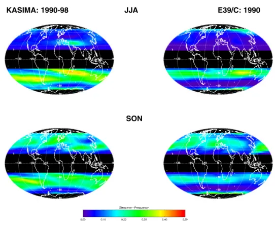
For both data sets, KASIMA and E39/C, the same meridional criterion for the iden-tification and counting of streamer events (Sect.2.1.1) has been used to derive clima-tologies. The resulting climatologies are presented in Fig.4.

3.2. Seasonal and geographical distribution of streamers

20

During December, January, and February (DJF; Fig. 4a) both climatologies indicate much higher streamer frequencies in the winter (northern) hemisphere than in the summer (southern) hemisphere. The horizontal distributions derived from KASIMA and E39/C both indicate a clear zonal asymmetry. There is an overall agreement with regard to the main activity centers which can be identified over the western part of

25

ACPD

Full Screen / Esc

Print Version

Interactive Discussion

c

EGU 2002

region. Individual years of the KASIMA analysis and the E39/C results do not differ significantly from each other, i.e. the climatological mean streamer distributions do not differ from those derived for cold (stable polar vortex) and warm (unstable polar vor-tex) winters (not shown). However, there are obvious quantitative differences between KASIMA and E39/C. E39/C generally simulates lower streamer frequencies during the

5

DJF season. This can also be seen in Fig.5. It shows the longitudinal distribution of the mean meridional (20◦N–70◦N) streamer frequency in the northern hemisphere. The maximum value is 0.23 at 0◦longitude in KASIMA, whereas it is only 0.17 in E39/C.

The streamer activity during March, April, and May (MAM; Fig. 4b) is notedly re-duced in the northern hemisphere (spring season) compared to DJF. Both

climatolo-10

gies indicate smaller frequency values. Higher values are found in the southern (fall) hemisphere, which are again systematically lower in E39/C. As in DJF in the northern hemisphere there is a satisfactory agreement between KASIMA and E39/C with regard to the main activity centers, except the western part of North America, where E39/C simulates nearly no streamers during this season. In the southern hemisphere the two

15

climatologies agree well not only qualitatively but also quantitatively.

Considering June, July, and August (JJA; Fig. 4c), the number of streamer events in the winter (southern) hemisphere is obviously higher than in the summer (northern) hemisphere in both climatologies which is qualitatively the same result as that found for DJF (e.g. higher frequencies in the winter season). Two centers of main

activ-20

ity are identified in the KASIMA and the E39/C climatologies, but they differ clearly with respect to the geographical location. KASIMA shows a pronounced center of ac-tion westward of the southern part of South America. In E39/C, this region is shifted northward. Moreover, the maximum frequency values are approximately a factor of 2 smaller than in KASIMA. The second region showing high streamer frequencies is

cen-25

tered above South Africa, whereas in E39/C it is shifted eastward and is located in the middle between South Africa and Australia. Again, the maximum values are smaller in E39/C. Generally, the streamer events simulated by E39/C are concentrated in a smaller latitudinal belt (20◦S–70◦S) as indicated by the KASIMA results. The much

ACPD

Full Screen / Esc

Print Version

Interactive Discussion

c

EGU 2002

higher streamer frequency in southern winter can also be seen in Fig.5, which indi-cates that the total number of streamer events counted in KASIMA is approximately a factor of two higher than in E39/C. The longitudinal variance of the mean merid-ional (20◦S–70◦S) streamer frequency in the southern hemisphere during winter time is smaller than in the northern winter season. In the northern hemisphere in summer,

5

the number of streamer events is very low in E39/C; it is considerably higher in KASIMA with a pronounced activity center east of the Mediterranean Sea, which is only weakly represented by E39/C (see Fig.4c).

For September, October, and November (SON) the differences between the KASIMA and the E39/C climatologies are largest in the southern hemisphere spring season

10

(Fig.4d). Here, the region of streamer activity in E39/C is simulated in a smaller latitudi-nal band than it is calculated by KASIMA. Also as was discussed for the other seasons, KASIMA results show higher values of streamer frequencies in both hemispheres, but it is most obvious in the southern hemisphere for this season. Nevertheless, the main center of activity which lies west of South America is identical for both climatologies.

15

In the northern hemisphere, the location of strongest activity are similar to those found during DJF.

A quantitative summary of the seasonal dependency of the mean streamer frequen-cies for 20◦–70◦ latitude in both hemispheres is given in Table 3, for KASIMA and E39/C, respectively. As formerly described, the frequency values derived from KASIMA

20

are larger than those calculated from E39/C, except for summer (DJF) and fall (MAM) conditions in the southern hemisphere. The differences between KASIMA and E39/C are most obvious during southern winter (JJA) and spring (SON) season. During sum-mer months, streasum-mer frequencies are smallest in both climatologies and both hemi-spheres.

25

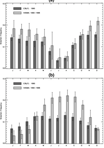
A closer inspection of the seasonal cycle of streamer frequencies on a monthly mean basis can be obtained from Fig.6. The annual cycle of the two models agree very well in the northern hemisphere. In the southern hemisphere there is a distinct discrepancy between the KASIMA analysis and the E39/C results especially for the period between

ACPD

Full Screen / Esc

Print Version

Interactive Discussion

c

EGU 2002

June and October indicating deficiencies in the dynamics of E39/C during that time. The annual cycle of the KASIMA streamer frequency climatology shows a clear sig-nature: maximum streamer frequencies are found near winter solstice (pronounced peak in December in the northern hemisphere) with a shift towards spring in the south-ern hemisphere (broad maximum from June to September). Interestingly, the

maxi-5

mum values are of the same order of magnitude in both hemispheres (approx. 0.22). Minimum streamer frequencies are detected in the months after summer solstice, i.e. July in the northern hemisphere and January in the southern hemisphere, with slightly higher values in the northern hemisphere (approx. 0.05 in the northern hemisphere, approx. 0.04 in the southern hemisphere). In summary, the shape of the annual cycle

10

of streamer frequencies seems to indicate a link to the seasonality of the stratospheric polar vortex.

Whereas the annual cycle of streamer frequencies in the northern hemisphere is in fair agreement between E39/C and KASIMA analysis (Fig.6), significant differences are found in the southern hemisphere for the months from June to October. At this time

15

of the year, E39/C, as most climate models, shows marked temperature deviations with respect to observations, a phenomenon known as the cold bias (Pawson et al.,2000;

Austin et al.,2002). In the model, the southern hemisphere winter and spring polar stratosphere is much too cold and the stratospheric vortex is too strong. An important question is how the cold bias of the model and the streamer climatology are related

20

to each other. Are both deficiencies of E39/C caused by the same missing (dynamic) process, or is the poor reproduction of streamer frequencies in winter and spring a direct consequence of the cold bias?

As mentioned above, the annual cycle of streamer events seems to be related to the dynamics of the stratosphere with high streamer activity in winter months. The

25

results presented here do not show higher frequency values during the formation or the decay of the polar vortex as shown in previously published analyses (e.g.Waugh,

1996). Moreover, for northern winter months neither the KASIMA analysis nor the re-sults of E39/C show different streamer frequencies in warm and cold winters, which

ACPD

Full Screen / Esc

Print Version

Interactive Discussion

c

EGU 2002

is also indicated by the relatively small standard deviations of the frequency values in winter (Fig. 6). Therefore, the dynamics of the polar vortex (stretching of the vortex, displacement from polar latitudes during a minor warming event, decay during a major stratospheric warming) seems not to be the primary process which forces streamer events in the analysed altitude region. Much more plausible is that large-scale

plan-5

etary (Rossby) waves which originate in the troposphere vertically propagate into the stratosphere and directly generate streamer events. From linear theory it follows that only during the west wind phase in the stratosphere (all seasons except summer) these waves can propagate upward from the troposphere into the stratosphere (Charney and

Drazin,1961). The upward propagation of those Rossby-waves and the breaking of

10

these waves at higher altitudes is one of the main causes for horizontal transport in that altitude range (e.g.Trepte et al.,1993;Chen et al.,1994;Waugh,1996). In E39/C, the deficiencies detected in the southern hemisphere might partly be caused by the horizontal resolution (T30) which may not be sufficient to resolve the relevant tropo-spheric dynamic processes which generate planetary waves there (see discussion

15

below). The systematic underestimation of (large-scale) wave activity in the south-ern hemisphere might be one reason for the cold bias (missing dynamical heating of the polar stratosphere), and it could also be the cause for the too small extra-tropical streamer frequencies in winter and spring season.

3.3. Discussion

20

The seasonal dependency of streamer activity found in KASIMA and E39/C partly agrees with formerly published studies (e.g. Chen et al., 1994; Waugh, 1996). For example, Chen et al. (1994) also found that the bulk of transport out of the tropics at the 600 K-level is into the winter hemisphere and only little transport into the sum-mer hemisphere. For winter in the northern hemisphere at the 400 K-level, Chen et

25

al. showed that roughly equal amounts of air masses are transported into both mid-latitudes, whereas during winter in the southern hemisphere most transport is found into southern hemisphere mid-latitudes.Waugh(1996) analysed the seasonal variation

ACPD

Full Screen / Esc

Print Version

Interactive Discussion

c

EGU 2002

of the isentropic transport out of the tropical stratosphere for the three-year period July 1991 to June 1994. Strong transport out of the tropics was found to occur whenever there are westerlies throughout middle latitudes, which is consistent with the KASIMA results. It was concluded that in the northern hemisphere the transport out of the trop-ics fluctuates about an approximately constant value during the fall to spring period

5

(late September to early May), a finding which is not supported by the current anal-ysis. A different result was also found in the southern hemisphere: Waugh detected maximum transport of air mass in early and late winter with a relatively quiet midwinter period. The KASIMA results do neither show an early and/or late winter maximum nor a reduced activity in mid-winter. Both studies (Chen et al.,1994;Waugh,1996) also

in-10

vestigated the altitude dependence of tropical mass exchange. Chen et al. showed that the tropics are most isolated in the middle stratosphere (600 K, approx. 25 km in the tropics) and that much more air of tropical origin is transported into mid-latitudes of the winter hemisphere in the upper (1100 K, approx. 38 km in the tropics) and lower (400 K, approx. 17 km in the tropics) stratosphere. Qualitatively, the same result was gained

15

by Waugh, considering 425 K, 500 K, and 850 K. A reasonable explanation for this behaviour was given by Chen and co-workers: in the lower stratosphere (tropopause region) there are more synoptic-scale waves originating in the troposphere than in the middle stratosphere (500–600 K) while the amplitude of planetary-scale disturbances in the upper stratosphere is much larger than in the middle stratosphere due to the

20

density effect. The findings discussed so far in the current paper, which are based on data only for altitudes between 21 and 25 km, fit well with this hypothesis, since we do not find a clear relation between the dynamics of the polar winter vortex and streamer events.

The identified seasonal cycle of streamer activity differs substantially from the one

25

derived by the SLIMCAT chemical transport model (Chipperfield,1999), where a period between February 1996 to February 1999 was analysed (Orsolini and Grant, 2000). The main difference is a higher activity in the summer season than in winter season in both hemispheres (Orsolini and Grant, 2000; their Fig. 2). In this study the vertical

ACPD

Full Screen / Esc

Print Version

Interactive Discussion

c

EGU 2002

streamer criterion discussed in Sect.2.1.2 was applied to the N₂O data. The altitude range between 500 and 600 K (roughly 20–25 km) was averaged. To examine the differences between the annual cycles of the KASIMA and the E39/C streamer clima-tologies presented in the current paper and the one of (Orsolini and Grant,2000), we have applied the same vertical criterion to the “1990” E39/C time slice experiment.

5

Surprisingly the resulting annual cycle is then in much better agreement with the SLIM-CAT study (not shown). In particular, we also find higher activity in the summer hemi-spheres, which conflicts with the climatologies derived with the meridional criterion. Since E39/C is able to reproduce the climatology obtained with SLIMCAT using the vertical criterion and the climatology derived with KASIMA using the meridional

crite-10

rion, it must be concluded that the differences in the climatologies are mainly due to the different criteria. The formal differences including an interpretation have already been described in Sect. 2.1. Therefore, an interpretation based on the expectation from the middle atmosphere circulation follows: It is well known from many climatologies (e.g.

CIRA,1992) that planetary wave activity is much smaller in summer than in winter, the

15

wave activity in northern hemisphere winter is larger than in southern hemisphere win-ter. Since planetary waves are a major cause for streamers (see Kouker et al., 1999a and references therein), it is expected from the arguments above that the streamer frequency is considerable larger in winter than in summer. Consequently the vertical criterion seems not to be appropriate for the detection of streamers.

20

In summary, although there are some differences with regards to formerly published analyses, the climatology of streamer frequencies based on KASIMA results seems to be reliable, not at last since it employs 9 years of ECMWF re-analysis and op-erational analyses. The agreement with the corresponding climatology derived from E39/C is satisfactory, except for winter and spring season in the southern hemisphere.

25

Therefore, in the following E39/C results of sensitivity experiments are used to assess possible changes in streamer distributions and frequencies related to climate change and to estimate the influence of streamers on the mid-latitude ozone budget.

ACPD

Full Screen / Esc

Print Version

Interactive Discussion

c

EGU 2002

4. Streamer activity in a changing climate

As shown before, streamer frequencies vary clearly with season, and streamers can significantly modify the ozone budget at mid-latitudes due to irreversible mixing of (sub-) tropical air (see Sect.5). This gives rise to the question, if the streamer frequencies are different in a changing climate. To get some first hints, four different time-slice

experi-5

ments of the past and future have been carried out (e.g.Hein et al.,2001;Schnadt et

al.,2002). They represent 1960, 1980, 1990 and 2015 conditions. Prescribed bound-ary conditions for the four simulations are given in Table2. Boundary values for the most important greenhouse gases (CO₂, N₂O, CH₄) for “1960”, “1980”, and “1990” are taken from (IPCC,1990), those for “2015” according to the IPCC-scenario IS92a

(busi-10

ness as usual,IPCC,1996). Upper boundary values for NO_y and ClX and the zonal CFC fields are adapted to observations for the present and past simulations and follow projected changes for “2015” (WMO,1999). Each model experiment was integrated for 20 model years. The model results representing recent atmospheric conditions have been intensively compared with respective observations. It turned out that the model is

15

able to simulate not only mean conditions in fair agreement with observations but also intra- and inter-annual changes of dynamic and chemical values and parameters, par-ticularly in the northern hemisphere. These findings have been taken as justification to employ E39/C also for an assessment of possible near future changes. The results of the four model experiments were provided for an international model inter-comparison

20

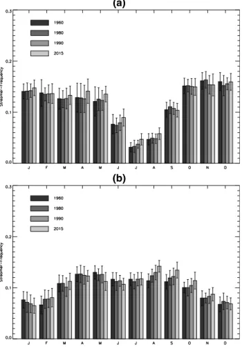
(Austin et al.,2002) which indicates the abilities and deficiencies of the currently used chemistry-climate models. Streamer climatologies for 1960, 1980, 1990 and 2015 for the altitude region from 21 to 25 km are shown in Fig.7.

First of all, it indicates no principle changes in the annual cycle, i.e. the maximum and minimum streamer frequencies in the four model simulations are always found in

25

the same months, they are not shifted to other months.

Comparing the results of the different time-slice simulations it is obvious that the inter-annual standard deviation (1 sigma) within a month of one specific model

experi-ACPD

Full Screen / Esc

Print Version

Interactive Discussion

c

EGU 2002

ment is mostly larger than the changes in streamer frequencies of one month between the four simulations. But there are a few exceptions which yield interesting facts: In both hemispheres, the streamer frequencies are found to increase in the summer months. Comparing the values of the “1960” and the “2015” simulations, this increase is statis-tically significant, for July in the northern hemisphere and for February in the southern

5

hemisphere, respectively. As already discussed bySchnadt et al. (2002), the model shows a systematic decrease of lower stratospheric temperatures in summer due to enhanced greenhouse gas concentrations which is in agreement with cooling trends estimated on the basis of long-term measurements (Ramaswamy et al., 2001). The cooling in the model is much more pronounced at high- than at mid- and low latitudes

10

(due to the decrease of polar ozone) which yields a reduced meridional temperature gradient in the extra-tropical lowermost stratosphere. This effect could be responsible for more streamer events since the lower stratosphere is more susceptible to synoptic-scale causing perturbations generated in the (sub-)tropical troposphere. Moreover, in a warmer troposphere, the generation of tropospheric waves could be different. Even

15

more synoptic-scale waves could be generated. Since easterly winds dominate the middle and upper stratosphere in summer (which is out of the model domain) and pre-vent the upward propagation of planetary waves, we expect no significant changes of streamer activity in that altitude region due to climate change.

A reduction of streamer frequencies in E39/C (from “1960” to “2015”) can be detected

20

in both hemispheres in early winter, i.e. in the months of maximum streamer activity. In the southern hemisphere a significant reduction of streamer frequencies is found in May; in the northern hemisphere a decrease of streamer events can be identified in November. Although the changes in the northern hemisphere are not statistically significant, it is interesting that again both hemispheres show the same behaviour.

25

Since both hemispheres react in the same way, stratospheric dynamics (variability) which are different in both hemispheres, especially in winter, might play a minor role in this altitude region (21–25 km). Another aspect supporting this theory is that the standard deviation of the streamer frequencies are of comparable magnitude in both

ACPD

Full Screen / Esc

Print Version

Interactive Discussion

c

EGU 2002

hemispheres. If stratospheric dynamics played a major role, the standard deviations should clearly be larger in the northern hemisphere.

The results presented in this section yield some interesting model behaviour. There are some first hints that the streamer frequency in both hemisphere might alter in a changing climate. This would certainly have an impact on the ozone budget at

mid-5

latitudes, and possibly small parts of the observed ozone changes in mid-latitudes in recent years could be related to changes in streamer activity. Some aspects sup-port the idea that dynamics of the stratospheric polar vortex might be of minor impor-tance and tropospheric dynamics could have a stronger impact on the development of streamers in the lower stratosphere. The results of this model study are not convincing

10

proofs but indications which are in line with formerly published investigations. Further analyses of long-term observations and respective model simulations are required to get more reliable conclusions.

5. Influence of streamers on mid-latitude ozone budget

Streamers, as discussed in the previous sections, transport tropical air masses to mid

15

and high latitudes, i.e. air masses, which are characterised by high N₂O and low ozone values compared to mid-latitude values. Therefore, they can reduce the ozone content in the mid-latitudes. In this section, we address two questions: (1) If these stream-ers had the same ozone mixing ratios like mid-latitude air masses, how much ozone would be additionally released in the mid-latitudes by streamers in comparison to the

20

photochemical ozone production? (2) Does this additional ozone have any impact on the mid-latitude ozone distribution via long-range transport? To answer these ques-tions we apply the coupled chemistry-climate model E39/C. We use a non-feedback (off-line) simulation of the 1990s (e.g.Hein et al.,2001;Grewe et al.,2001) and com-pare it with the results of a sensitivity simulation, where we fill-up streamers with ozone

25

according to the surrounding air masses. Three years are analysed after a spin-up period of 2 years. A feedback of the ozone changes on the dynamics is excluded in

ACPD

Full Screen / Esc

Print Version

Interactive Discussion

c

EGU 2002

either simulation, i.e. they have identical meteorology. By comparing the results of this simulation with those of the standard 1990 simulation, we are able to detect and to quantify the effects of streamers on the ozone distribution. For these simulations the detection criterion has to be adapted, since not only a change of the N₂O gradient has to be detected (point 1 in Fig.2), but also the point where N₂O reaches the mid-latitude

5

value again (point 2), which is the first poleward data point with at least the same N₂O value like point 1. Between these points 1 and 2 ozone values are linearly interpolated and adjusted to this value whenever the actual ozone mixing ratio is less than this in-terpolated value (shaded area II in Fig. 2). This criterion is then applied to 7 model levels, which represent approximately 30 to 100 hPa.

10

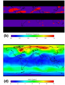
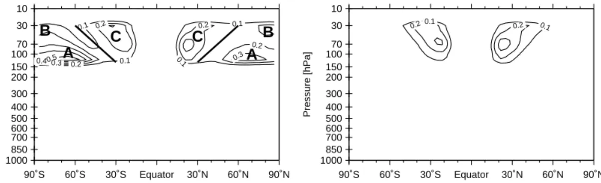
Figure 8 (left) shows the frequency of streamers detected in the E39/C simulation. Applying the on-line detection without any regional restrictions results in the detection of different phenomena as streamers (see Sect. 2.1.1). By scanning sequences of latitude and longitude plots of N₂O, and the streamer frequency at different heights, three regions were detected in each hemisphere, which have the same characteristics

15

like streamers, in terms of the meridional gradient of N₂O. A region A, where upper tropospheric high pressure systems lead to a high tropopause and disturbances of the stratospheric N₂O field, which are not related to streamers. A region B, which is influenced by the polar vortex. Cut-offs of the polar vortex and also displacements of the polar vortex can lead to similar structures of the meridional gradient of N₂O, which

20

are also not related to streamers. And a region C, which finally is characterised by streamers. The characterisation has been done on a daily basis for 4 representative months of each season. To avoid an impact of these high pressure systems and of the polar vortex, in the following we only concentrate on the region C and we are aware that we may loose some streamers, which can reach to high latitudes. Therefore, this

25

on-line detection should lead to a lower boundary of the number of streamers and the chemical effects.

Figure8(right) clearly shows the vertical structure of streamer events, with a maxi-mum at 70 hPa and decreasing values above, agreeing well with previous findings (see

ACPD

Full Screen / Esc

Print Version

Interactive Discussion

c

EGU 2002

Sect. 3.3). It also indicates a tendency of higher streamer frequencies with deep pole-ward intrusion at higher altitudes. The air masses detected between 30 and 100 hPa during a year amount to 155.5 · 1015 kg (Table 4) with higher contributions from the northern hemisphere than from the southern hemisphere. The seasonal cycle in the southern hemisphere is much less pronounced than in the northern hemisphere.

Min-5

imum (maximum) values are found in the spring (fall) season of both hemispheres. However, this result is largely dominated by the streamer events at lower altitudes (60 to 100 hPa), which represent around 65% of all detected streamers (30 to 100 hPa). At higher altitudes (30 to 40 hPa) streamers mainly transport air masses into the winter hemisphere (NH for DJF and SH for JJA) with a very pronounced seasonal cycle. The

10

region 30 to 50 hPa (approx. 21–25 km) shows the same with a less pronounced sea-sonal cycle, though. Below 60 hPa this air mass exchange pattern changes: Streamers transport more mass into the summer hemisphere. As expected, the results for the al-titude region 30 to 50 hPa (Table4) confirm the results presented in Table3.

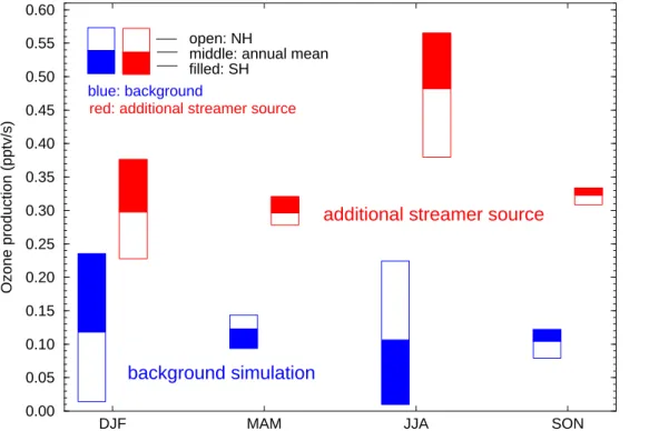
The additional ozone source in the perturbation simulation depends on two factors

15

(see Fig.9), the detected air volume (Table 4) and the surrounding ozone concentra-tion. The larger the detected volume the more ozone is released in the perturbation simulation and the flatter the latitudinal ozone gradient the less ozone is released. This artificial source has the same pattern as the streamer frequency (Fig.10, shaded ar-eas). Figure9shows the strength of the photochemical ozone source in the region of

20

the streamers in comparison to the streamer ozone source. In general, the mean pho-tochemical ozone source (photolysis of O₂and subsequent reaction with O₂) of 0.10 to 0.12 pptv/s is smaller in all seasons than this artificial streamer ozone source of 0.30 to 0.48 pptv/s. The region, where streamers occur, i.e. around 70 hPa at mid-latitudes (Fig. 8), is characterised by minimal ozone production. The hemispheric deviations

25

from mean photochemical ozone production are quite large and mirror the variations of the solar zenith angle. The hemispheric variations in the streamer ozone source are much less pronounced. In all seasons, more ozone is released in northern hemisphere streamers than in the southern hemisphere.

ACPD

Full Screen / Esc

Print Version

Interactive Discussion

c

EGU 2002

The comparison of the simulation with the additional ozone source with the standard simulations is presented in Fig. 10. The additional ozone source affects the ozone concentration only below 40 hPa. In the region above that height the short lifetime inhibits a transport of the ozone perturbation. Two regions with maximum perturbation can be found at around 100 hPa and 20◦N and 20◦S, resulting from the location of

5

the additional ozone source and the maximum of the ozone lifetime at 100 hPa. The ozone released in the streamers yields an increase in the mid-latitude lowermost strato-sphere of 100% in the winter hemistrato-sphere and around 75% in the summer hemistrato-sphere. Stratosphere-troposphere exchange leads to an increase of tropospheric ozone values of roughly 40 to 50% in the southern winter hemisphere (JJA) and 50 to 75% in the

10

northern winter hemisphere (DJF). In the summer hemisphere and in the tropics, ver-tical mixing (convection) leads to a faster destruction of ozone yielding an increase of roughly 30%.

From our simulations it seems that the importance of the streamers for the ozone concentration strongly depends on the altitude of the steamer occurrences. The

addi-15

tional streamer ozone at around 25 km (30 hPa) lead to an increase in the order of 1 to 5%, whereas at around 15 km (100 hPa) it can be as high as 400%, which means that locally ozone can be reduced by 80% through streamer mass exchange. Conse-quently, the lowermost stratosphere and the ozone content is not only determined by stratospheric ozone transported downwards from the stratosphere, but also by ozone

20

at tropical tropopause levels transported towards higher latitudes. At the tropopause ozone increases by roughly 40% in the summer hemispheres and 100% in the winter hemispheres. This means that streamers lead to a decrease of approximately 30% and 50% of the ozone at the tropopause in the standard simulation for summer and winter hemispheres, respectively. Other sources of the tropopause ozone budget are

25

the polar stratosphere, the troposphere, as well as in situ ozone production, e.g. by nitrogen oxides from tropical lightning (Grewe et al.,2002).

ACPD

Full Screen / Esc

Print Version

Interactive Discussion

c

EGU 2002

6. Conclusions

A new criterion has been applied to establish a climatology of streamer frequencies. For the first time, a 9 year data record has been used to get more reliable information about the geographical distribution and the annual cycle of streamer activity in the al-titude region from 21 to 25 km. The results from the KASIMA model, which employs

5

ECMWF re-analyses between 1990 and 1994 and operational analyses thereafter until 1998, show a pronounced seasonal dependence of streamer activity with highest quency values in northern mid-winter and late southern winter. Very low streamer fre-quencies have been found during summer months in both hemispheres. The KASIMA climatology has been employed to evaluate the corresponding results of the coupled

10

chemistry-climate model E39/C. It shows a satisfactory agreement, except for south-ern winter and spring conditions where E39/C clearly underestimates the number of streamer events. Neither the streamer frequency climatology of KASIMA nor that of E39/C indicate strong standard deviations, in particular not for northern winter, i.e. the streamer frequencies and also the geographical distribution do not differ for different

15

stratospheric conditions, i.e. years with a cold and stable polar vortex and those with a warm and unstable polar vortex. This indicates that the direct impact of the dynam-ics of the stratospheric polar vortex, which is well described by E39/C (Hein et al.,

2001), is weak for the generation and development of streamers in the lower strato-sphere. In agreement with formerly published investigations (e.g. Chen et al.,1994;

20

Waugh,1996) it seems that synoptic-scale waves originating in the troposphere are the main drivers for streamer events in the lower stratosphere. This gives an impor-tant hint for the possible origin of the cold bias in E39/C, which is also found in late winter and spring, especially in the southern hemisphere. The coarse horizontal res-olution of E39/C (i.e. T30) probably hinders the adequate forcing and development of

25

synoptic-scale waves (stationary and transient eddies) and their vertical propagation into the middle atmosphere. In the northern hemisphere, this model deficiency might be partly compensated due to the consideration of the effects of orographic gravity

ACPD

Full Screen / Esc

Print Version

Interactive Discussion

c

EGU 2002

waves, which do not play such an important role in the southern hemisphere, yielding more realistic heat and momentum fluxes (Schnadt et al.,2002). As a consequence, planetary wave activity in the southern hemisphere of E39/C, although weak, is under-estimated considerably. Therefore, we believe that the cold bias of E39/C in the south polar region in winter and spring and the obvious underestimation of streamer activity

5

in the lower stratosphere during this time of the year, do have the same origin, i.e. the model does not adequately simulate tropospheric synoptic-scale waves in the southern hemisphere.

In literature (e.g.Tibaldi et al.,1990;Hamilton et al.,1999) clear hints have been pre-sented that higher horizontal and vertical model resolutions reduce the (extra-tropical)

10

cold bias in climate models at all stratospheric heights, particularly in the southern hemisphere. In the extra-tropical troposphere, low resolution models (e.g. T21) show a different behaviour from higher resolution models (T42 or even higher), for example, a too weak southern hemisphere zonal flow, or horizontal momentum fluxes which are underestimated in both hemispheres. In Hein et al. (2001) it could be demonstrated

15

that increasing the number of vertical model layers from 19 to 39 in ECHAM/CHEM while keeping the horizontal model resolution constant (T30), yields a much better rep-resentation of lower stratospheric dynamics, especially in the northern hemisphere. For example, E39/C shows a satisfactory dynamic variability with cold and stable polar winters as well as warm winters including pronounced warming events. Further model

20

studies are required to give more reliable information about the relation between tropo-spheric wave forcing, streamer activity in the lower stratosphere, and the cold bias in climate models.

The climate change sensitivity studies employing E39/C do not indicate dramatic changes, neither the geographical distribution of streamer activity nor the number of

25

streamer events. The seasonal cycle does not change in the different simulations (“1960”, “1980”, “1990”, and “2015”), i.e. low streamer activity is always found in sum-mer and maximum activity in winter. A slight increase of streasum-mer frequencies is simu-lated for summer months and a reduction of streamer activity in winter, comparing the

ACPD

Full Screen / Esc

Print Version

Interactive Discussion

c

EGU 2002

frequency values of the “1960” simulation with those of “2015”. Although these changes are partly significant, they cannot explain larger parts of observed mid-latitude ozone reduction, which have been underestimated in most models.

Sensitivity experiments with E39/C have been used to assess the impact of stream-ers on the ozone budget at mid-latitudes. As found in recent investigations, an altitude

5

dependency of the mass of streamers has been indicated by E39/C results. A simple model assessment shows that the effects of streamers on the mid-latitude ozone dis-tribution have much larger impacts in the lower stratosphere than in the middle strato-sphere. The decrease of ozone at around 25 km is of the order of less than 5% whereas at around 15 km it can reach 80%. Therefore, it is obvious that a realistic simulation of

10

streamers (amount, distribution, seasonal cycle) in CCMs is necessary to calculate the ozone budget at mid-latitudes in a realistic way. The current study indicates that this requires an adequate representation of horizontal transport processes.

Acknowledgements. We thank Thilo Erbertseder, Jens-Uwe Groos, Rolf M ¨uller and Thomas

Reddmann for helpful discussions, Christoph Br ¨uhl, Michael Ponater, Roland Ruhnke and

15

Christina Schnadt for their comments on the orginal manuscript and Bernd Sch ¨aler for pro-viding the CRISTA data. This work was supported by the ENVISAT validation project of the HGF-Vernetzungsfonds sponsored by the German government (BMBF).

References

Appenzeller, C. and Holton, J. R.: Tracer lamination in the stratosphere: A global climatology,

20

J. Geophys. Res., 102, 13 555–13 569, 1997. 2304

Austin, J., Shindell, D., Beagley, S. R., Br ¨uhl, C.. Dameris, M., Manzini, E., Nagashima, T., Newman, P., Pawson, S., Pitari, G., Rozanov, E., Schnadt, C., and Shepherd, T. G.: Uncer-tainties and assessments of chemistry-climate models of the stratosphere, Atmos. Chem. Phys. Discuss., 2, 1035–1096, 2002. 2310,2314

25

Becker, G., M ¨uller, R., McKenna, D. S., Rex, M., and Carslaw, K. S.: Ozone loss rates in the arctic stratosphere in the winter 1991/92: model calculations compared with Match results, Geophys. Res. Lett., 25, 4325–4328, 1998. 2301

ACPD

Full Screen / Esc

Print Version

Interactive Discussion

c

EGU 2002

Brinkop, S. and Roeckner, E.: Sensitivity of a general circulation model to parameterisation of cloud-turbulence interaction in the atmospheric boundary layer, Tellus, 47A, 197–220, 1995.

2306

CIRA: COSPAR International Reference Atmosphere, Akademie Verlag, Berlin, 1986. 2313

Charney, J. P. and Drazin, P. G.: Propagation of planetary-scale disturbances from the lower

5

stratosphere into the upper atmosphere, J. Geophys. Res., 66, 83–109, 1961. 2311

Chen, P., Holton, J. R., O’Neill, A., and Swinbank, R.: Isentropic mass exchange between the tropics and extratropics in the stratosphere, J. Atmos. Sci., 51, 3006–3018, 1994. 2300,

2311,2312,2320

Chipperfield, M. P.: Multiannual simulations with a three-dimensional chemical transport model,

10

J. Geophys. Res., 104, 1781–1805, 1999. 2312

Dameris, M., Nodorp, D., and Sausen, R.: Correlation analysis of tropopause height and TOMS-data for the EASOE-winter 1991/1992, Contr. Atmos. Phys., 68, 227–232, 1995.

2299

Ehhalt, D. H., R ¨oth, E. P., and Schmidt, U.: On the temporal variance of stratospheric trace gas

15

concentrations, JAC, 1, 27–51, 1983. 2304

Fouquart, Y. and Bonnel, B.: Computations of solar heating of the Earth’s atmosphere: a new parameterisation, Beitr. Phys. Atmosph., 53, 35–62, 1980. 2306

Grewe, V. and Dameris, M.: Calculating the global mass exchange between stratosphere and troposphere, Ann. Geophysicae, 14, 431–442, 1996. 2299

20

Grewe, V., Dameris, M., Sausen, R., and Steil, B.: Impact of stratospheric dynamics and chem-istry in northern hemisphere mid-latitude ozone loss, J. Geophys. Res., 103, 25 417–25 433, 1998. 2301

Grewe, V., Dameris, M., Hein, R., Sausen, R., and Steil, B.: Future changes of the atmospheric composition and the impact of climate change, Tellus, 53B, 103–121, 2001. 2316

25

Grewe, V., Reithmeier, C., and Shindell, D. T.: Dynamical-chemical coupling of the upper tropo-sphere and lower stratotropo-sphere region, Chemotropo-sphere: Global Change Science, 47, 851–861, 2002. 2319

Hamilton, K., Wilson, R. J., and Hemler, R. S.: Middle atmosphere simulated with high vertical and horizontal resolution versions of a GCM: improvements in the cold bias and generation

30

of a QBO-like oscillation in the tropics, J. Atmos. Sci., 56, 3829–3846, 1999. 2321

Hein, R., Dameris, M., Schnadt, C., Land, C., Grewe, V., K ¨ohler, I., Ponater, M., Sausen, R., Steil, B., Landgraf, J., and Br ¨uhl, C.: Results of an interactively coupled chemistry-general

ACPD

Full Screen / Esc

Print Version

Interactive Discussion

c

EGU 2002

circulation model: Comparison with observations, Ann. Geophysicae, 19, 435–457, 2001.

2306,2307,2314,2316,2320,2321

Holton, J. R., Haynes, P. H., McIntyre, M. E., Douglas, A.R., Rood, R. B., and Pfister, L.: Stratosphere-troposphere exchange, Rev. Geophys., 33, 403–439, 1995. 2299

IPCC: (Intergovernmental Panel on Climate Change) Climate change, The IPCC Scientific

As-5

sessment, (Eds) Houghton, J. T., et al., Cambridge University Press, Cambridge, UK, 1990.

2314

IPCC: (Intergovernmental Panel on Climate Change) Climate change 1995, The science of climate change, (Eds) Houghton, J. T., et al., Cambridge University Press, Cambridge, UK, 1996. 2314

10

Kouker, W., Beck, A., Fischer, H., and Petzoldt, K.: Downward transport in the upper strato-sphere during the minor warming in February 1979, J. Geophys. Res., 100, 11 069–11 084, 1995. 2305

Kouker, W., Offermann, D., K¨ull, V., Reddmann, T., and Franzen, A.: Streamers observed by the CRISTA experiment and the KASIMA model, J. Geophys. Res., 104, 16 405–16 418, 1999a.

15

2300,2305

Kouker, W., Langbein, I., Reddmann, T., and Ruhnke, R.: The Karlsruhe Simulation Model of the Middle Atmosphere (KASIMA), Version 2, Forsch. Karlsruhe, Wiss. Ber No. 6278, Karlsruhe, Germany, 1999b. 2305

Kowol-Santen, J., Elbern, H., and Ebel, A.: Estimation of cross-tropopause airmass fluxes at

20

midlatitudes: comparison of different numerical methods and meteorological situations, Mon. Wea. Rev., 128, 4045–4057, 2000. 2299

Land, C., Ponater, M., Sausen, R., and Roeckner, E.: The ECHAM4.L39(DLR) atmosphere GCM – technical description and model climatology, Report No. 1991-31, DLR Oberpfa ffen-hofen, Wessling, Germany, ISSN 1434-8454, 1999. 2306

25

Louis, F.-J.: A parametric model of vertical eddy fluxes in the atmosphere, Boundary-Layer Meteorol., 17, 187–202, 1979. 2306

Manney, G. L., Michelsen, H. A., Irion, F. W., Toon, G. C., Gunson, M. R., and Roche, A. E.: Lamination and polar vortex development in fall from ATMOS long-lived trace gases oberserved during November 1994, J. Geophys. Res., 105, 29 023–29 038, 2000. 2303

30

Miller, M. J., Palmer, T. N., and Swinbank, R.: Parameterisation and influence of sub-grid scale orography in general circulation and numerical weather prediction models, Meteorol. Atmos. Phys., 40, 84–109, 1989. 2306