HAL Id: hal-00296295
https://hal.archives-ouvertes.fr/hal-00296295
Submitted on 24 Jul 2007
HAL is a multi-disciplinary open access
archive for the deposit and dissemination of
sci-entific research documents, whether they are
pub-lished or not. The documents may come from
teaching and research institutions in France or
abroad, or from public or private research centers.
L’archive ouverte pluridisciplinaire HAL, est
destinée au dépôt et à la diffusion de documents
scientifiques de niveau recherche, publiés ou non,
émanant des établissements d’enseignement et de
recherche français ou étrangers, des laboratoires
publics ou privés.
U. Schumann, H. Huntrieser
To cite this version:
U. Schumann, H. Huntrieser. The global lightning-induced nitrogen oxides source. Atmospheric
Chemistry and Physics, European Geosciences Union, 2007, 7 (14), pp.3823-3907. �hal-00296295�
www.atmos-chem-phys.net/7/3823/2007/ © Author(s) 2007. This work is licensed under a Creative Commons License.
Chemistry
and Physics
The global lightning-induced nitrogen oxides source
U. Schumann and H. HuntrieserDeutsches Zentrum f¨ur Luft- und Raumfahrt, Institut f¨ur Physik der Atmosph¨are, Oberpfaffenhofen, 82230 Wessling, Germany
Received: 16 January 2007 – Published in Atmos. Chem. Phys. Discuss.: 22 February 2007 Revised: 24 May 2007 – Accepted: 9 July 2007 – Published: 24 July 2007
Abstract. The knowledge of the lightning-induced nitro-gen oxides (LNOx) source is important for understanding and predicting the nitrogen oxides and ozone distributions in the troposphere and their trends, the oxidising capacity of the atmosphere, and the lifetime of trace gases destroyed by reactions with OH. This knowledge is further required for the assessment of other important NOx sources, in par-ticular from aviation emissions, the stratosphere, and from surface sources, and for understanding the possible feedback between climate changes and lightning. This paper reviews more than 3 decades of research. The review includes labo-ratory studies as well as surface, airborne and satellite-based observations of lightning and of NOxand related species in the atmosphere. Relevant data available from measurements in regions with strong LNOxinfluence are identified, includ-ing recent observations at midlatitudes and over tropical con-tinents where most lightning occurs. Various methods to model LNOxat cloud scales or globally are described. Previ-ous estimates are re-evaluated using the global annual mean flash frequency of 44±5 s−1 reported from OTD satellite data. From the review, mainly of airborne measurements near thunderstorms and cloud-resolving models, we conclude that a “typical” thunderstorm flash produces 15 (2–40)×1025NO molecules per flash, equivalent to 250 mol NOxor 3.5 kg of N mass per flash with uncertainty factor from 0.13 to 2.7. Mainly as a result of global model studies for various LNOx parameterisations tested with related observations, the best estimate of the annual global LNOx nitrogen mass source and its uncertainty range is (5±3) Tg a−1 in this study. In spite of a smaller global flash rate, the best estimate is es-sentially the same as in some earlier reviews, implying larger flash-specific NOxemissions. The paper estimates the LNOx accuracy required for various applications and lays out strate-gies for improving estimates in the future. An accuracy of Correspondence to: U. Schumann
about 1 Tg a−1or 20%, as necessary in particular for under-standing tropical tropospheric chemistry, is still a challeng-ing goal.
1 Introduction
Thunderstorm lightning has been considered a major source of nitrogen oxides (NOx, i.e. NO (nitric oxide) and NO2 (nitrogen dioxide)) since von Liebig (1827) proposed it as a natural mechanism for the fixation of atmospheric nitro-gen (Hutchinson, 1954). Lightning-induced nitronitro-gen oxides (LNOx) have several important implications for atmospheric chemistry and climate (WMO, 1999; IPCC, 2001). The global LNOxsource is one of the largest natural sources of NOxin the atmosphere (Galloway et al., 2004) and certainly the largest source of NOxin the upper troposphere, in partic-ular in the tropics (WMO, 1999).
The LNOxsource rate is considered to be the least known one within the total atmospheric NOxbudget (Lawrence et al., 1995; Lee et al., 1997). The global LNOxamount can-not be measured directly, and is difficult to determine. Mod-elling of the horizontal and vertical distribution of lightning and the LNOx source is highly uncertain (Price and Rind, 1992; Pickering et al., 1998). Previous reviews of LNOx dis-cuss theoretical, laboratory, and field studies to determine the amount of LNOx(Tuck, 1976; Drapcho et al., 1983; Borucki and Chameides, 1984; Biazar and McNider, 1995; Lawrence et al., 1995; Levy II et al., 1996; Lee et al., 1997; Price et al., 1997b; Huntrieser et al., 1998; Bradshaw et al., 2000; Ri-dley et al., 2005), mainly by extrapolating measurements of emissions from individual lightning or thunderstorm events to the global scale (Chameides et al., 1977, 1987). Only a few papers review the determination of the global LNOx source by fitting models to observations (Levy II et al., 1996; Zhang et al., 2003b). The majority of studies since the mid-1990s, as reviewed in this paper, assumed a best-estimate
NOx mixing ratio, nmol mol-1 0.001 0.01 0.1 1 10 O H co n ce n tra ti o n , 1 0 5 cm -3 0 1 2 3 4 N e t O3 p ro d u ct io n ra te , 1 0 4 cm -3 s -1 0 2 4 6 8 OH P(O3) 4 μ
Fig. 1. Dependence of the OH concentration and the net O3
pro-duction rate on the NOxmixing ratio calculated with a steady state
box model for diurnal average in June at 10 km altitude and 45◦ latitude; background mixing ratios of O3: 100 nmol mol−1; H2O:
47 µmol mol−1; CO: 120 nmol mol−1; CH4: 1660 nmol mol−1;
re-plotted from Ehhalt and Rohrer (1994) with kind permission of Woodhead Publishing Limited.
value of about 5 Tg a−1(NOxsource values are given in ni-trogen mass units per year in this paper), with an uncertainty range 1–20 Tg a−1. Extreme estimates of the LNO
xsource rate such as 0.2 Tg a−1(Cook et al., 2000) and 220 Tg a−1 (Franzblau and Popp, 1989; Liaw et al., 1990), implying the global LNOxcontribution from minor to overwhelming, are now considered inconsistent with measured atmospheric NOx concentrations and nitrate deposition values (Gallardo and Rodhe, 1997).
Considerable progress has been made recently which al-lows reducing the uncertainty of the global LNOxvalue. This includes satellite observations of global lightning (Christian et al., 2003), satellite observations of NO2column distribu-tions (Burrows et al., 1999), airborne in-situ measurements of NOxabundance near thunderstorms at midlatitudes (Dye et al., 2000; Huntrieser et al., 2002; Ridley et al., 2004) and over tropical continents, where most lightning occurs (see Sect. 2.4), detailed cloud-resolving model studies (DeCaria et al., 2000; Fehr et al., 2004), and improved global models (Dentener et al., 2006; van Noije et al., 2006).
This paper reviews the present knowledge on the global LNOx source rate. It describes the importance of NOx for tropospheric chemistry (Sect. 2.1). It reviews knowledge on the NOx concentrations, sources and sinks (Sect. 2.2), the essential lightning properties (Sect. 2.3), and the forma-tion of NOx from lightning and its detection in the atmo-sphere (Sect. 2.4). It briefly summarises knowledge on the formation of other trace gases by lightning (Sect. 2.5). It describes the importance of LNOx for tropospheric chem-istry and its impact on ozone (Sect. 2.6). Moreover, it as-sesses the global modelling of NOxand LNOxdistributions (Sect. 2.7), the possible climate impact of LNOx (2.8), the
relative importance of aviation NOxfor uncertain LNOx con-tributions (Sect. 2.9), and derives requirements on LNOx ac-curacy (Sect. 2.10). Thereafter, the paper reviews the various methods to constrain the LNOxsource values (Sect. 3). It re-evaluates results from flash (Sect. 3.1) and storm (Sect. 3.2) extrapolations using the most recent satellite observations of the global lightning frequency. In addition, the paper reviews for the first time the results of a large number of global model studies discussing LNOximpact on tropospheric chemistry (Sect. 3.3). Section 3.3 also elaborates on the potential of better constraining the LNOx source estimate using global model fits to observations of concentrations and deposition fluxes of nitrogen compounds and other species. Finally, Sect. 4 presents the conclusions.
2 Review of LNOxcontributions and their importance
2.1 Importance of NOxfor atmospheric chemistry
Nitrogen oxides are critical components of the troposphere which directly affect the abundance of ozone (O3) (Crutzen, 1974) and the hydroxyl radical (OH) (Levy II, 1971; Rohrer and Berresheim, 2006). Ozone is known as a strong oxidant, a strong absorber of ultraviolet radiation, and a greenhouse gas (WMO, 1999). Ozone is formed and destroyed by pho-tochemistry and the net production rate depends nonlinearly on the abundance of NOx present (Liu, 1977), see Fig. 1. In regions with low NOx level (e.g. in the tropical marine boundary layer), the net effect is an O3 destruction. In re-gions with NOxconcentrations above a critical level (but not very high), e.g. in the upper troposphere, O3production dom-inates. The critical NOxlevel depends on the O3mixing ratio and may be as low as 5 pmol mol−1in the oceanic boundary layer with typically low ozone values (Crutzen, 1979), 10– 50 pmol mol−1in the free troposphere (Fishman et al., 1979; Ehhalt and Rohrer, 1994; Brasseur et al., 1996; Davis et al., 1996; Kondo et al., 2003b), and increases with the ambient O3concentration (Grooß et al., 1998). Hence, in regions re-mote from strong local pollution, O3 production increases with NOxconcentration (is “NOxlimited”). The relative in-crease of O3production is largest for low NOx concentra-tions.
The concentrations of HOx including OH, the hydroper-oxyl radical HO2and other peroxy radicals, depend also non-linearly on the NOx abundance (Logan et al., 1981; Ehhalt and Rohrer, 1994; Jaegl´e et al., 1999; Olson et al., 2006), see again Fig. 1. Under clean air conditions, OH is mainly produced by O3 photolysis and reactions of the resultant atomic oxygen with water vapour. Under more polluted con-ditions in the troposphere, OH is also formed by photoly-sis of NO2during the oxidation of carbon monoxide (CO), methane (CH4) and non-methane hydrocarbons (NMHC). In highly polluted regions (in “NOx-saturated” regions) an in-crease of NOx, by reactions with HO2and NO2, reduces the
Table 1. Best estimate of LNOxand total NOxemissions in reviews and assessments.
Reference Best estimate of LNOxsource rate (and range)
in nitrogen mass, in Tg a−1
Total NOx emissions in
ni-trogen mass, in Tg a−1
for year
Tuck (1976) 4 –
Chameides et al. (1977) 30–40 –
Dawson (1980) 3 –
Ehhalt and Drummond (1982) 5 (2–8) 39 (19–59) 1975
Logan (1983) 8 (2–20) 50±25 1980
Borucki and Chameides (1984) 2.6 (0.8–8) –
IPCC (1992) 2–20 35–79
Lawrence et al. (1995) 2 (1–8) 60
Levy et al. (1996) 4 (2–6) –
Price et al. (1997a, b) 12–13 (5–25) –
Lee et al. (1997) 5 (2–20) 44 (23–81) 1980
Huntrieser et al. (1998) 4 (0.3–22) –
WMO (1999) 5 (2–20) 44 (30–73) 1990s
Ehhalt (1999) 7 (4–10) 45±7 1990
Holland et al. (1999a) 13 (10–15) 36.1 (23–81) 1980s
Bradshaw et al. (2000) 6.5 (2–10) 45.2 (27–86) 1985 IPCC (2001) 5 (2–13) 52 (>44) 2000 Leue et al. (2001) – 43±20 1997 Tie et al. (2002) 3.5–7 – Huntrieser et al. (2002) 3 (1–20) – Martin et al. (2003) – 44.4 1997 Galloway et al. (2004) 5.4 13.1, 46, 82 1860, 1990s, 2050
M¨uller and Stavrakou (2005) 2.8 (1.6–3.2) 42.1 (38.8–43.1) 1997
Boersma et al. (2005) 3.5 (1.1–6.4) –
Law et al. (2006) 2–9 –
Present estimate 5±3 (2–8) –
HO2/OH ratio, and the production rate of O3(Jaegl´e et al., 1999, 2001). OH is the key agent in the atmosphere’s oxi-dising capacity, i.e. the global abundance of tropospheric O3, OH, and hydrogen peroxide (H2O2) (Crutzen, 1979; Logan et al., 1981; Isaksen, 1988; Thompson, 1992; Lelieveld et al., 2004). OH influences the lifetime of a large number of anthropogenic and natural compounds. Here, lifetime is the ratio between the amount of the species and its sinks. Ex-amples are CO (Logan et al., 1981), sulphur dioxide (SO2) (Chatfield and Crutzen, 1984), CH4 (Lelieveld et al., 1998; Bousquet et al., 2006), and further O3and aerosol precursors or gases relevant to climate that get oxidised by reactions with OH. As a consequence, NOxincreases not only cause a positive radiative forcing implying warming via O3(Lacis et al., 1990) but also a cooling via CH4; the forcing from these effects is of similar magnitude globally but differs regionally (Fuglestvedt et al., 1999).
2.2 NOxsources, sinks, and concentrations
The concentration of NOx in the atmosphere depends on the source strength and the rates of reactions converting NOx to nitric acid (HNO3) and particulate nitrate (NO−3) and their uptake into precipitation or deposition at the Earth surface (Crutzen, 1979; Warneck, 1988; Dentener and Crutzen, 1993; Ehhalt, 1999). NO and NO2 are together referred to as NOx because NO reacts in the atmosphere quickly with O3to form NO2and equilibrium with respect to photodissociation of NO2is reached after a few minutes, while the sum of both species remains essentially unchanged (Bradshaw et al., 1999). Collectively, all reactive odd nitrogen or fixed nitrogen is denoted as NOy, which is any N-O combination except the very stable N2O, i.e. NO+NO2+NO3+2N2O5+HNO3+HNO2+HNO4+PAN+ RONO2+NO−3, including PAN (peroxyacetylnitrate, RC(O)OONO2) and alkyl nitrates (RONO2) (Singh et al., 2007). Conversion of unreactive N2 to more reactive nitrogen NOy occurs in the biosphere and the atmosphere (Galloway et al., 2004).
Table 2. Annual global NOxemissions, in the tropics, and at midlatitudes (in Tg a−1).
Latitude range Biomass Fossil fuel Soil N2O Aviation Lightning Sum∗ Lightning Reference burning burning release degradation NOx fraction, %
90◦S–90◦N 10.0 28.5 5.5 0.4 0.7 5.0 49.4 10 See footnote∗∗∗ 35◦N–60◦N 0.7 13.7 1.5 0 0.4 14.1 4 ∗∗∗
35◦S–35◦N 9.2 13.6 3.9 0.4 0.3 4.3 31.3 14 ∗∗∗
35◦S–35◦N 8.3 7.8 5.4 – – 6.3 27.9 23 Bond et al. (2002)∗∗ 0◦–24◦S 4.4 1.2 1.5 0 0.03 1.7 8.8 19 ∗∗∗
∗All emission rates in nitrogen mass per year (Tg a−1). ∗∗
Bond et al. (2002): Fossil fuel (“anthropogenic activity”), biomass burning and soil emissions from EDGAR 2.0, year 1990 (Olivier et al., 1998), lightning NOxcomputed from LIS flash data over the period of 1998-2000 assuming production values of 6.7×1026and 6.7×1025
NO molecules for each CG and IC flash, respectively.
∗∗∗Biomass burning (including waste and biofuel burning); and fossil fuel burning (including industrial emissions but without the AERO2K aviation part) derived from the EDGAR 3.2 Fast Track 2000 dataset (Olivier et al., 2005); Soil release from the Global Emissions Inventory Activity (GEIA; 5.4 Tg a−1) (Benkovitz et al., 1996); aviation sources for 2002 from the AERO2K data set (Eyers et al., 2005); stratospheric
source from N2O degradation for an assumed 0.4 Tg a−1 total (Martin et al., 2006) and downward transport according to
stratosphere-troposphere exchange mainly near the subtropical jet (Grewe and Dameris, 1996; Stohl et al., 2003). Lightning NOxcomputed from the
five-year (April 1995–March 2000) OTD 2.5 Degree Low Resolution Diurnal Climatology data, assuming constant NOxproduction per flash
and a total LNOxsource of 5 Tg a−1.
Latitude, °N -60 -40 -20 0 20 40 60 80 N it ro g e n e mi ssi o n , T g a -1 d e g re e -1 0.0 0.2 0.4 0.6 0.8 1.0 1.2 + Fossil + Biomass + Soil LNOx 2 3
Fig. 2. Atmospheric annual nitrogen mass emission rate per 1◦ lat-itude versus latlat-itude for the year 2000. Lightning emissions are tentatively computed from satellite (OTD)-derived flash frequencies (Christian et al., 2003) (see Fig. 10), assuming constant emissions per flash and 5 Tg a−1global LNOxemissions. Added to this: soil
emissions derived from Yienger and Levy (1995) with data taken from the Global Emissions Inventory Activity (GEIA; 5.4 Tg a−1)
(Granier et al., 2004); biomass burning (including waste and bio-fuel burning; 10 Tg a−1); and fossil fuel burning (including
indus-trial emissions; 28.5 Tg a−1) derived from the Emission Database
for Global Atmospheric Research (EDGAR) (Olivier et al., 2005).
In the atmosphere, the present sources of global NOx (to-tal about 50 Tg a−1), see Table 1, are dominated by
anthro-pogenic sources from fossil fuel combustion (about 28–32) (IPCC, 2001), biomass burning (4–24), soil (4–16) (Lee et
al., 1997), nitrous oxide (N2O) degradation in the strato-sphere (0.1–1) (Lee et al., 1997; Martin et al., 2006), air-craft (0.7–1) (Schumann et al., 2001; Eyers et al., 2005), and LNOx. Most of the emissions occur in the Northern Hemisphere, see Table 2 and Fig. 2. Ship NOx emissions, presently about 3–6 Tg a−1(Eyring et al., 2005; Olivier et al., 2005), are included in the fossil fuel combustion source; they represent an important marine source along the major ship routes. In the preindustrial period, natural sources from soil processes, wildfires (biomass burning), stratospheric sources and LNOxdominated the budget: For the year 1860, the to-tal NOx emissions are estimated as 13.1 Tg a−1, including 5.4 Tg a−1from LNO
xand 5.1 Tg a−1from the other natural sources (Galloway et al., 2004).
The principal sink of tropospheric NOxis oxidation to ni-tric acid (HNO3) by reaction of NO2 with OH during the day; during the night, the reaction of NO2with O3to form NO3, the oxidation of NO2by NO3to form N2O5, and the subsequent hydrolysis of N2O5on aerosols contributes con-siderably to the nitrogen oxides sinks (Dentener and Crutzen, 1993; van Noije et al., 2006). The oxidation products leave the atmosphere by dry or wet deposition (“acid rain”) (Lo-gan, 1983). When deposited they may act as nutrients in terrestrial and marine ecosystems (Holland et al., 1997), and may disturb ecologically sensitive regions such as the Ama-zon basin, central Africa, south-east Asia (Sanderson et al., 2006), and India (Kulshrestha et al., 2005).
Until the early 1980s very few measurements of nitro-gen oxides in the atmosphere were available (Kley et al., 1981; Warneck, 1988; Bradshaw et al., 2000). Whereas NO2columns can be measured locally from ground (Noxon, 1976), from space in terms of the optical absorption of solar
Table 3. Airborne air composition measurement experiments in regions with lightning contributions.
Acronym∗ Region Altitudes,
km
Time Period References
– Frankfurt (Germany) to S˜ao Paulo (Brazil)
along east coast of Brazil
10.7 Dec 1982 Dickerson (1984)
GTE/CITE 1A Central North Pacific around Hawaii 9 Nov 1983 Chameides et al. (1987); Davis et al. (1987)
STRATOZ III 55◦N–55◦S, passing over South America 12 June 1984 Drummond et al. (1988)
PRE-STORM Southern Great Plains, Colorado 0–12 June 1985 Dickerson et al. (1987); Luke et al. (1992)
GTE/ ABLE 2A Amazon Basin, Brazil 0–5 Aug 1985 Gregory et al. (1988); Torres et al. (1988); Hoell
(1999)
GTE/CITE 2 East N. Pacific and Continental U.S. 8 Aug–Sep 1986 H¨ubler et al. (1992)
STEP Tropical region near Darwin, Australia 11 Jan–Feb 1987 Murphy et al. (1993); Pickering et al. (1993);
Russell et al. (1993)
NDTP North Dakota, USA 10.8–12.2 28 June 1989 Poulida et al. (1996)
ELCHEM New Mexico, USA 6–12 July–Aug 1989 Ridley et al. (1994, 1996)
TROPOZ II 55◦N–55◦S, passing South America 0–11 Jan-Feb 1991 Rohrer et al. (1997); Jonquieres and Marenco
(1998)
PEM-West A West North Pacific (0◦–45◦N) 0–12 Oct 1991 Crawford et al. (1996); Gregory et al. (1996);
Singh et al. (1996)
GTE/TRACE-A Brazil and South Atlantic (0◦–30◦S) 8–12 Sep–Oct 1992
(dry season)
Fishman et al. (1996); Pickering et al. (1996); Smyth et al. (1996a)
PEM-West B 30◦N–10◦S, West Pacific, Guam – Hong Kong 8.9–12 Feb 1994 Gregory et al. (1997); Kawakami et al. (1997);
Singh et al. (1998)
POLINAT I and II West Europe and North Atlantic 0–12 Nov 1994,
June–July 1995, Aug–Nov 1997
Schlager et al. (1997, 1999); Schumann et al. (2000)
NOXAR I and II Airliner routes between Zurich (Switzerland)
and Atlanta (USA), and Beijing (China)
6–11 1995–1997 Brunner (1998); Jeker et al. (2000); Brunner et
al. (2001)
SUCCESS North America 0–12.5 April–May 1996 Jaegl´e et al. (1998)
STERAO North-Eastern Colorado 2–11 June–July 1996 Stith et al. (1999); Dye et al. (2000)
LINOX Southern Germany and Switzerland 0–10 July 1996 Huntrieser et al. (1998); H¨oller et al. (1999)
PEM Tropics A Sep 1996 Gregory et al. (1999);
PEM-Tropics-A-Science-Team (1999)
SONEX USA and North Atlantic 0–11 Oct–Nov 1997 Singh et al. (1999); Crawford et al. (2000);
Thompson et al. (2000b)
EULINOX Germany and Southern Europe 1–10 July 1998 H¨oller and Schumann (2000); H¨oller et
al. (2000); Huntrieser et al. (2002)
MOZAIC Airliners routes between mid Europe and South
Africa, South America and Far East
0–12 1998–2005 Marenco et al. (1998); Volz-Thomas et al. (2005)
STREAM 98 Canada 7.5–13 July 1998 Lange et al. (2001)
BIBLE Tropical western Pacific and Australia 1–14 Sep–Oct 1998,
Aug–Sep 1999, Nov–Dec 2000
Kondo et al. (2003a); Koike et al. (2007)
INCA 55◦N–55◦S, passing South America 0–12 March–April
2000
Baehr et al. (2003); Schumann et al. (2004a)
CONTRACE West Europe 0–12 Nov 2001–July
2003
Huntrieser et al. (2005)
SPURT 35–75◦N, 10◦W–20◦E 0–13.7 Nov 2001–July
2003
Engel et al. (2006)
CRYSTAL-FACE Florida, USA 8–18 July 2002 Ridley et al. (2004)
HIBISCUS Brazil, and tropical tropopause region 10–23 Feb–March
2004
Pommereau et al. (2007)
TROCCINOX 2004 and 2005 Between Europe and Brazil, and local flights
near State of Sao Paulo
0–12.5 and 0–20 Jan–March 2004, and Jan–Feb 2005 Schumann et al. (2004b); Huntrieser et al. (2007); http://www.pa.op.dlr.de/troccinox/
INTEX-A/ICARTT/ITOP North America, North Atlantic and West
Eu-rope
0–12.8 July–Aug 2004 Fehsenfeld et al. (2006); Singh et al. (2006)
CARIBIC Airliner routes between mid Europe and South
Africa, South America and Far East
0–12 2005 Brenninkmeijer et al. (2005, 2007)
SCOUT-O3 Between Europe and Darwin, Australia, and
lo-cal flights in the Hector cloud north of Darwin
0–20 Nov–Dec 2005 http://www.ozone-sec.ch.cam.ac.uk/scout o3
ACTIVE and TWPICE Area around Darwin, Australia 0–20 Nov 2005–
March 2006
http://www.atm.ch.cam.ac.uk/active/ http://www.bom.gov.au/bmrc/wefor/research/ twpice.htm
AMMA Area around Ouagadougou, Burkina Faso, West
Africa
Table 3. Continued.
∗) ACTIVE: Aerosol and Chemical Transport in Tropical Convection; AMMA: African Monsoon Multidisciplinary Analysis; BIBLE: Biomass Burning and Lightning Experiment; CARIBIC: Civil Aircraft for the Regular Investigation of the Atmosphere Based on an Instru-mented Container; CONTRACE: Convective Transport of Trace Gases into the Middle and Upper Troposphere over Europe: Budget and Impact on Chemistry; CRYSTAL-FACE: The Cirrus Regional Study of Tropical Anvils and Cirrus Layers - Florida Area Cirrus Experiment; ELCHEM: Electrified Cloud Chemistry; EULINOX: European Lightning Nitrogen Oxides Experiment; GTE/ABLE 2A; Global Tropo-spheric Experiment/Amazon Boundary Layer Experiment 2A; GTE CITE: Global TropoTropo-spheric Experiment – Chemical Instrumentation Test and Evaluation; GTE/TRACE-A: Global Tropospheric Experiment/Transport and Chemistry Near the Equator – Atlantic; HIBISCUS: Impact of tropical convection on the upper troposphere and lower stratosphere at global scale; ICARTT: International Consortium for Atmo-spheric Research on Transport and Transformation; INCA: InterhemiAtmo-spheric Differences in Cirrus Properties from Anthropogenic Emissions; INTEX-A: Intercontinental Chemical Transport Experiment – North America; ITOP: Intercontinental Transport of Ozone and Precursors; LINOX: Lightning Nitrogen Oxides Experiment; MOZAIC: Measurement of Ozone by Airbus in-service Aircraft; NDTP: North Dakota Thunderstorm Project; NOXAR II: Nitrogen Oxides and Ozone along Air Routes; PEM: Pacific Exploratory Mission; POLINAT: Pollution in the North Atlantic flight corridor; PRE-STORM: Preliminary Regional Experiment for STORM-CENTRAL; SCOUT-O3: Stratospheric-Climate Links with Emphasis on the Upper Troposphere and Lower Stratosphere; SONEX: Subsonic Assessment, Ozone and Nitrogen Oxide Experiment; SPURT: Spurenstofftransport in der Tropopausenregion; STEP: Stratosphere Troposphere Exchange Project; STERAO: Stratosphere – Troposphere Experiment – Radiation, Aerosols and Ozone; STRATOZ III: Stratospheric Ozone Experiment; STREAM: Stratosphere-Troposphere Experiment by Aircraft Measurements; SUCCESS: Subsonic aircraft: Contrail and cloud effects special study; TROCCINOX: Tropical Convection, Cirrus, and Nitrogen Oxides Experiment; TROPOZ II: Tropospheric Ozone Experiment; TWPICE: Tropical Warm Pool International Cloud Experiment.
Table 4. Nitrogen oxides chemical lifetimes (in days) in various atmospheric regions.
Altitude range, km Global(1) North America(2) Western North Pacific(3) South Atlantic Basin(4) Tropical South Pacific(5)
2–4 1 0.3–0.8 1.1–1.8 0.18 0.7–1
4–8 5 1–3 1.5–2.4 0.66 1.1–2.1
8–12 10 3–10 3.2–8.9 2.4 4.2–7.4
(1)Tropospheric regions which have not recently experienced deep convection. Based on MATCH-MPIC model results (Lawrence et al., 2003b; von Kuhlmann et al., 2003b). The three altitude ranges given correspond to the lower troposphere, middle troposphere and upper troposphere in the model.
(2)Photochemical model constrained to data obtained during SUCCESS over North America in April and May (Jaegl´e et al., 1998). (3)Western North Pacific, 0–42◦N, photochemical model constrained with observed NO, O
3, H2O, CO, NMHC, H2, CH4, temperature,
pressure, and UV solar flux values (PEM West A). In this analysis, the NOxlifetime decreases with latitude. The lower/upper bounds given
reflect the values for 18–42◦N and 0–18◦N, respectively (Davis et al., 1996).
(4)South Atlantic Basin. Model for the Southern Hemisphere TRACE-A data (Jacob et al., 1996; Smyth et al., 1996b). (5)Tropical South Pacific (PEM-Tropics A), photochemical model constrained with observations (Schultz et al., 1999).
light in limb (Russell III et al., 1993; Llewellyn et al., 2004; Rind et al., 2005) and nadir (Burrows et al., 1999; Zhang et al., 2000), tropospheric NO cannot be determined by remote sensing accurately. In recent decades, in-situ instruments to measure NO, NOx, and NOyand their speciation accurately at low and high concentrations have been developed (Clemit-shaw, 2004; Singh et al., 2007). Accurate in-situ measure-ments of NO are difficult to perform, because of the large range of concentrations and the large spatial and temporal variability. Many in-situ instruments determine the NO con-centration from the rate of photon emissions from chemilu-minescence (CL) during reaction of NO with excess O3in a reaction chamber; NOyis measured similarly after catalytic conversion of NOyto NO (Fahey et al., 1985; H¨ubler et al., 1992; Bradshaw et al., 1998). Alternatively, NO may be
measured with low detection limits using two-photon laser-induced fluorescence (TP-LIF) (Sandholm et al., 1990) and NO2with a time-gated laser-induced fluorescence instrument (LIF) (Thornton et al., 2000).
Since the early 1980s, many airborne field experiments have been carried out to measure NOx and NOy compo-nents in the free troposphere (Bradshaw et al., 2000; Em-mons et al., 2000; Brunner et al., 2001), see Table 3. Sev-eral experiments obtained measurements of NOx, O3, ozone precursors, aerosols and air mass tracers in convective out-flow regions. But only a few dedicated experiments (such as STERAO, LINOX, EULINOX, and TROCCINOX) mea-sured these species in the inflow and outflow regions of the storms together with measurements of the cloud structure and kinematics and the lightning activity, which can be used to
NOX (ppbv) 0.0 0.2 0.4 0.6 0.8 1.0 1.2 1.4 A lt it ude (m ) 0 2000 4000 6000 8000 10000 12000 NO/NOX 0.0 0.2 0.4 0.6 0.8 1.0 EULINOX EULINOX (a) (b)
Fig. 3. Average profiles of (a) NOxconcentration and (b) NO/NOxratio (Huntrieser et al., 2002). The profiles represent the mean values over
all EULINOX mission days (except the case of 21 July, with an exceptionally strong thunderstorm). The horizontal bars indicate standard deviations.
connect the chemical measurements in the convective out-flow to specific cloud and lightning properties.
The atmospheric NOxmole fraction or mixing ratio (i.e. number of NOx molecules per number of air molecules) spans a wide range (0.001–100 nmol mol−1) and shows
con-siderable small-scale spatial and temporal variability due to local sources and highly variable sinks. The mixing ratio values reach from an order of 1–10 pmol mol−1in the clean maritime boundary layer to an order of 10–100 nmol mol−1 in polluted continental boundary layers (Fehsenfeld and Liu, 1993; Carroll and Thompson, 1995). It reaches an or-der of 0.05–1 nmol mol−1 near the tropopause, and about 20 nmol mol−1 near 3 hPa pressure altitude in the tropical stratosphere (Grooß and Russell III, 2005). The tropospheric vertical profile often shows a C-shape with low values in the mid-troposphere and high values in the polluted boundary layer and near the tropopause (Kley et al., 1981; Drummond et al., 1988; Warneck, 1988; Luke et al., 1992; Rohrer et al., 1997; Huntrieser et al., 2002), see for example Fig. 3a. Up-per tropospheric NOxstems from fast vertical transport from the planetary boundary layer via convection, downward mix-ing of stratospheric sources, and from in-situ sources from lightning and aviation (Ehhalt et al., 1992; Schlager et al., 1997; Thompson et al., 2000b). The equilibrium ratio of NO/NOx increases with the NO2 photolysis rate, and de-creases with the ambient O3concentration and ambient tem-perature (Schlager et al., 1997); hence, it varies typically be-tween 0.3 and 0.9 during day time (Fig. 3b), with the largest values above clouds in the upper tropical troposphere, and approaches zero quickly during night.
The lifetime for NOxwith respect to photochemical loss, see Table 4 and a plot in Levy et al. (1999), varies between 0.2 and 10 days, generally increasing with latitude and
alti-tude in the troposphere; the lifetime of NO2 is shorter than that of NO (Davis et al., 1996). The lifetime of HNO3against photolysis is of the order of 10 to 20 days in the tropics and increases strongly with latitude (Jacob et al., 1996; Tie et al., 2001). HNO3rainout occurs intermittently in precipitation events (Giorgi and Chameides, 1985; Giannakopoulos et al., 1999; Shindell et al., 2006). In the troposphere, part of the NOxgets converted to PAN which is thermally unstable, not water-soluble, and has a long lifetime in the cold upper tro-posphere (100 days at −30◦C) (Tie et al., 2001). As a
conse-quence, the tropospheric NOx/NOyratio varies strongly, typ-ically from 0.05 to 0.5 (Ridley et al., 1994; Singh et al., 1996; Ziereis et al., 2000; Koike et al., 2003; Hegglin et al., 2006). This ratio is often larger than in photochemical equilibrium with HNO3 and PAN, suggesting fresh NOx sources from convection and lightning (Jaegl´e et al., 1998; Ko et al., 2003; Koike et al., 2003). In the upper troposphere over the North Atlantic, the NOycomposition was found to be dominated by a mixture of NOx(25%), HNO3(35%) and PAN (17%) (Talbot et al., 1999). Over North America in summer, NOx contributes about 15% to NOy, while PAN and HNO3are the dominant species, providing some 65% of NOy, with PAN dominating in the upper troposphere and HNO3in the lower troposphere (Singh et al., 2007). In the upper troposphere, the NOx/HNO3ratio varies strongly because convection pro-vides local sources of NOx while HNO3 is depleted due to scavenging during uplift (Jaegl´e et al., 1998). In the tropical Pacific, convection has been observed to increase NOxover land and to decrease NOxover the ocean because of upward transport of polluted or very clean air masses, respectively (Koike et al., 2003). The NOx/HNO3 ratio has been used to test the validity of photochemical models and as “chem-ical clock” to determine the age of air since outflow from
Table 5. Satellite platforms and instruments providing NO2column measurements.
Instrument∗ Satellite Period Spatial
resolu-tion, km2
Local time at equator
Swath, km Global cover after, days
Spectral range, nm
Reference
GOME ERS-2 1995–2003∗∗ 320×40 10:30 a.m. 960 3 240–790 Burrows et al. (1999) SCIAMACHY ENVISAT Since 2002 60×30 10:00 a.m. 960 6 240–2380 Bovensmann et al. (1999) OMI AURA Since 2004 13×24 01:45 p.m. 2600 1 270–500 Levelt et al. (2006) GOME-2 METOP Since Oct 2006 80×40 09:30 a.m. 1920 1.5 240–790 Munro et al. (2006)
∗AURA: NASA Earth Science satellite; ENVISAT: European Earth Observation satellite; ERS-2: European Remote Sensing Satellite; GOME (-2): Global Ozone Monitoring Experiment (-2); METOP: ESA – Polar orbiting weather satellite; OMI: Ozone Monitoring Instru-ment; SCIAMACHY: Scanning Imaging Absorption Spectrometer for Atmospheric Cartography.
∗∗GOME continued measurements with reduced spatial coverage thereafter.
NOy, nmol mol-1
0.01 0.1 1
O3, nmol mol-1
0 20 40 60
CO, nmol mol-1 0 20 40 60 80 100 NOx, nmol mol-1
0.001 0.01 0.1 A lt it u d e , k m 2 4 6 8 10 12
INCA Punta Arenas INCA Prestwick NOXAR 1995 POLINAT 1997
Fig. 4. Trace gas profiles from airborne measurement flights out of Punta Arenas in March 2000 and Prestwick in September 2000 dur-ing the project INCA (Baehr et al., 2003). For comparison median values of POLINAT II (Shannon, Ireland, July–September 1997) (Schumann et al., 2000) and NOXAR 1995 (>50◦N) (Brunner et al., 2001) are included. Symbols and whiskers indicate median val-ues and 25% and 75% percentiles, respectively.
convective clouds (Prather and Jacob, 1997; Schultz et al., 1999; Wang et al., 2000; Bertram et al., 2007).
Because of the different magnitudes of the NOx emis-sions, tropospheric concentrations are higher over the con-tinents than over the oceans (Drummond et al., 1988), and higher at northern than at southern midlatitudes (Baehr et al., 2003), see Fig. 4. First climatologies of NOx and NOy (Carroll and Thompson, 1995; Emmons et al., 1997; Thakur et al., 1999) have been considerably extended by the Nitro-gen Oxide and Ozone Concentration Measurements along Air Routes (NOXAR) project. The measurements in the up-per troposphere at Northern midlatitudes show background NOxvalues in the 20–200 pmol mol−1range, highly skewed probability distributions, and large regions with NOx > 0.5 nmol mol−1reflecting fresh sources from upward con-vection of polluted boundary layer air masses and lightning contributions (Brunner et al., 2001), see Fig. 5.
Measurements of NO2profiles from space have been ob-tained by limb sounding methods, e.g., the Halogen Oc-cultation Experiment (HALOE) (Russell III et al., 1993), SAGE II (Stratospheric Aerosol and Gas Experiment II) (McCormick, 1987), the Michelson Interferometer for Pas-sive Atmospheric Sounding (MIPAS) (Funke et al., 2005), and the Optical Spectrograph and Infrared Imager System (OSIRIS) (Llewellyn et al., 2004). These instruments pro-vide profiles versus altitude and latitude in the stratosphere and in the upper troposphere above clouds. NO2 columns above the Earth surface can be derived from nadir measure-ments. Data on the global distribution of NO2columns have been provided by the Global Ozone Monitoring Experiment GOME since 1995 (Burrows et al., 1999), and later by SCIA-MACHY (Bovensmann et al., 1999), and OMI (Levelt et al., 2006); GOME-2 on METOP was launched recently, see Ta-ble 5. The GOME and SCIAMACHY satellite overpasses are restricted to the morning hours (10:00 or 10:30 LT), when the LNOxsource is small (Kurz and Grewe, 2002). Better spatial coverage and observations during the early afternoon is pro-vided by OMI (Bucsela et al., 2006). Measurements on such low orbiting satellites suffer the effects of cosmic radiation when passing the South Atlantic anomaly of the geomagnetic field off the coast of Southern Brazil (Heirtzler, 2002).
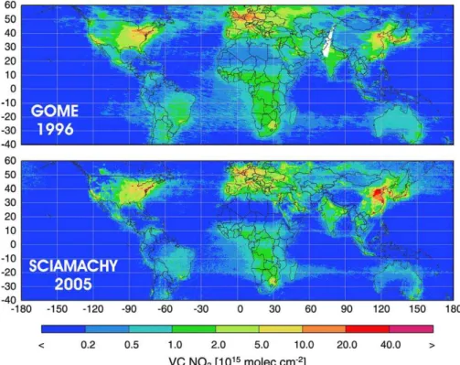
The total NO2 molecule column amounts to about 1.5– 3×1015cm−2in the tropics and 0.5–6×1015cm−2at middle and high latitudes (Wenig et al., 2004). The stratospheric part is rather smooth longitudinally and dominates in remote oceanic regions with low local pollution. Therefore, the tro-pospheric part, see Fig. 6, may be obtained by subtracting the total column in such remote regions. The tropospheric NO2column may reach a maximum of up to 50×1015cm−2 locally at 30×60 km2resolution over the industrial regions in the annual mean. In the tropics the NO2plumes originate from the continents, presumably mainly from biomass burn-ing, soil emissions and local pollution near large cities. The tropospheric column of NO2molecules per unit surface area is dominated by the NO2abundance in the lower troposphere. The presence of clouds prevents the detection of NO2below the cloud, and enhances detection of NO2above cloud top.
1
Fig. 5. Distribution of NOxmixing ratio in the 330–220 hPa altitude range in the four seasons (a: MAM, b: JJA, c: SON, d: DJF). Numbers
denote the sample sizes along the routes (Brunner, 1998).
The satellite-derived NO2 columns have been used to-gether with estimates of the NO2lifetime or with global
mod-els to derive global or regional NOx budgets (Leue et al., 2001; Velders et al., 2001; Lauer et al., 2002; Martin et al.,
1
2 3
Fig. 6. Annual mean tropospheric NO2column density versus longitude and latitude from a retrieval of, top: GOME data for the year 1996;
bottom: SCIAMACHY data for the year 2005. The data and the analysis method are described in Richter et al. (2005). Figure provided by A. Richter (personal communication, 2006).
2002a; Richter and Burrows, 2002; Duncan et al., 2003; Ed-wards et al., 2003; Kunhikrishnan et al., 2004; Savage et al., 2004; Choi et al., 2005; Irie et al., 2005; Jaegl´e et al., 2005; Konovalov et al., 2005; Meyer-Arnek et al., 2005; Richter et al., 2005; Ma et al., 2006; van der A et al., 2006; van Noije et al., 2006). Figure 6 illustrates the improvement in spatial res-olution provided by SCIAMACHY compared to GOME. On the other hand, the GOME time series is still longer. GOME and SCIAMACHY data have been used to detect decreases of NO2column values over Europe and the USA and increases over China (Richter et al., 2005), which are obvious from Fig. 6. Moreover, GOME and SCIAMACHY data have been used successfully to detect ship-NOx emissions, in spite of their small NO2columns of the order of (0.5–1)×1015cm−2 (Beirle et al., 2004a; Richter et al., 2004).
The LNOxcontribution to the NO2column is difficult to observe directly from space for various reasons (Hild et al., 2002; Choi et al., 2003; Beirle et al., 2004b; Martin et al., 2006). Any correlation between NO2 columns and light-ning frequency densities is not immediately evident. Dif-ferent methods of GOME retrievals vary by more than 10% (van Noije et al., 2006). Therefore, accurate LNOxestimates require LNOxcolumn contributions significantly larger than 10%. Model studies compute LNOxcontributions to the NO2 column below (2–6)×1014 molecules cm−2 (Martin et al., 2003, 2007; Boersma et al., 2005), i.e. a small fraction of the
annual mean NO2column even in the tropics. The computed LNOxcolumn contribution is generally below 20% (Martin et al., 2003; Boersma et al., 2005; van Noije et al., 2006) with localized fractions of more than 80% in regions with weak surface NOx emissions (Martin et al., 2007). Detections of LNOxcontributions to the NO2column in space-based ob-servations are discussed in Sect. 2.4.
2.3 Lightning
Lightning is a transient, high-current electric discharge over a path length of several kilometres in the atmosphere (Uman, 1987). The majority of lightning in the Earth’s atmosphere is associated with convective thunderstorms (MacGorman and Rust, 1998; Rakov and Uman, 2003). Lightning forms from the breakdown of charge separation in thunderstorms. Charge separation is efficient for strong updrafts containing supercooled liquid water, ice crystals and hail or graupel (Takahashi, 1984; Saunders, 1993; Deierling et al., 2005; Petersen et al., 2005; Kuhlman et al., 2006; Sherwood et al., 2006). The charge separation leads to high electric field strengths in thunderstorms (Marshall et al., 1995). Once the electric field exceeds a certain threshold value, a light-ning discharge may occur (Stolzenburg et al., 2007). The threshold value decreases with altitude and is of the order of 100 to 400 kV m−1, far smaller than in the laboratory,
2
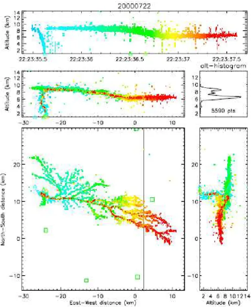
3
Fig. 7. Radiation sources for a negative CG discharge observed within STEPS. The colours indicate time progression, and the different panels show the evolution of the flash in (top) height-time, (bottom left) plan view, and in (middle left) east-west (E-W) and (bottom right) north-south (N-S) vertical projections. Also shown is a histogram of the source heights. The triangles indicate negative ground strike times and locations from the National Lightning Detection Network (NLDN). The squares in the plan view indicate the location of measurement stations, and the vertical line denotes the Colorado-Kansas state border; from Thomas et al. (2004).
possibly because of cosmic-ray-induced electrical break-down in the atmosphere (Dwyer, 2005; Gurevich and Zy-bin, 2005; Khaerdinov et al., 2005). The lightning discharge in its totality is called a flash (Orville, 1968). One distin-guishes between cloud-to-ground (CG) lightning and vari-ous other lightning types (which we call IC), including intr-acloud, intercloud and cloud-to-air lightning. So-called blue jets have been observed above clouds, and sprites and other transient luminescent events occur in the middle atmosphere (F¨ullekrug et al., 2006). Positive and negative CG flashes (CG+ and CG-) are distinguished depending on whether pos-itive or negative charges are transported from the cloud to the ground. CG+ discharges are less frequent than negative ones,
but have larger currents and transfer more charge (Orville, 1994; Lyons et al., 1998b). Lightning occurs typically in a sequence of stages. A CG discharge begins with local dielec-tric breakdown causing first branched conduction paths in-side the cloud. The breakdown initiates conducting channels, e.g. in the form of a “stepped leader” that moves earthward in discrete steps. A large fraction of charge is lowered to the ground within a “return stroke,” an intense discharge region that propagates up the stepped leader path from ground to cloud. A flash consists of one or more strokes closely spaced in time travelling along the same discharge channel (Thery, 2001; Saba et al., 2006a). The first stroke is often the most energetic one and assumed to produce the largest amount of
LNOx (Hill, 1979; Dawson, 1980). Large currents also oc-cur in relatively slow discharge processes, such as continuing currents, in both cloud and cloud-to-ground flashes (Rakov and Uman, 2003; Saba et al., 2006b). The flash proper-ties vary from storm to storm and during the lifecycle of a thunderstorm; they depend on the volume and strength of the convective updrafts causing charge separation (Lang and Rutledge, 2002); as well, they depend on the degree of cell isolation and the complexity of cell evolution (MacGorman et al., 2007).
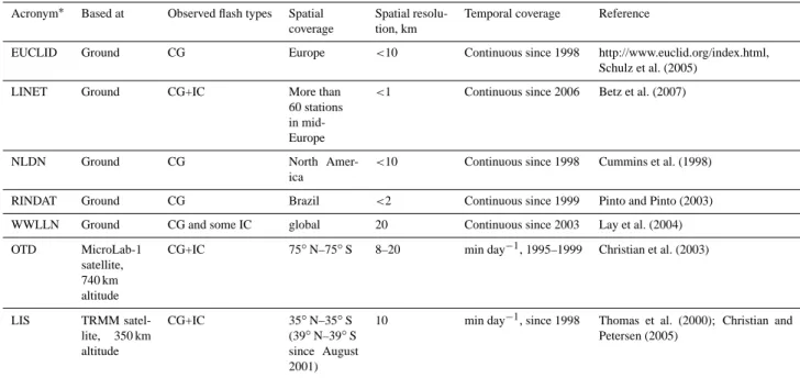
Lightning can be detected from ground and from space using sensors measuring the optical emission, electric radio waves, or magnetic waves resulting from the discharge pro-cesses in certain frequency ranges (MacGorman and Rust, 1998). The low frequency (LF, 30–300 kHz), very low fre-quency (VLF, 3–30 kHz), extremely low frefre-quency (ELF, 30–300 Hz), and very high frequency (VHF, 30–300 MHz) bands are employed for lightning detection besides acous-tical and opacous-tical detection means. Various parts of a flash cause different emissions. The bright spark of light associ-ated with CG lightning stems from the return stroke. Light-ning channels behave like a huge antenna which radiates electromagnetic energy as signals of impulsive nature be-low about 100 kHz (Price et al., 2007). Strong LF radio emission is generated by CG flashes mainly near ground. IC flashes emit multi-pulse bursts of VHF signals from the inner parts of the clouds (Proctor, 1991; Suszcynsky et al., 2000; Thomas et al., 2000). The continuing current between strokes causes small radio wave signals but large reductions in the electric field strength. Most of the ground-based opera-tional lightning detection networks provide two-dimensional (2-D) maps of mainly CG lightning events (Orville et al., 2002) (Table 6). Regionally, within a dense network of detec-tors, height information is also available (Table 7). The sys-tems use magnetic direction finders (Cummins et al., 1998), time of arrival (Shao and Krehbiel, 1996) or VHF interfer-ometers techniques (Defer et al., 2001) to evaluate the loca-tion of the lightning sources. In addiloca-tion, the duraloca-tion, and energy or peak current of the flash can be deduced from the measured electromagnetic signals. The peak current is ap-proximately proportional to the amplitude of VLF/LF signals (Orville, 1999; Jerauld et al., 2005; Schulz et al., 2005). Peak current measurements are sensitive to network station spac-ing; recent measurements show median peak currents of the order of 16–20 kA, smaller than what was estimated earlier (Orville et al., 2002; Biagi et al., 2007).
VHF systems allow for fine-scale observations of the structure of flashes. For example, Fig. 7 shows a light-ning discharge observed by the VHF New Mexico Tech Lightning Mapping Array (LMA, see Table 7) (Noble et al., 2004; Thomas et al., 2004; Wiens et al., 2005) dur-ing the Severe Thunderstorm Electrification and Precipita-tion Study (STEPS) (Lang et al., 2004), that illustrates the spatial resolution that the system is able to obtain. Simulta-neous data from the National Lightning Detection Network
(NLDN) show that the flash was a multiple-stroke negative CG discharge. The top panel of the figure shows the alti-tude of the VHF sources versus time and indicates an initial stepped leader initiated between 8 and 9 km altitude, after about 50 ms of preliminary breakdown, that required about 60 ms to reach the ground. Thomas et al. (2004) show that the location accuracy for VHF sources between about 6 and 12 km altitude over the central part of the network is <12 m in horizontal position and <30 m in the vertical.
Since the mid 1980s ground-based observations have provided detailed information on the structure of VLF/LF sources radiated by lightning in real time with regional cov-erage. In many countries lightning detection is routinely per-formed by means of VLF/LF-networks. Prominent examples are the NLDN in the USA and EUCLID in Europe. These systems report mainly strong (>5 kA) CG strokes (Cum-mins et al., 1998). Advanced VLF/LF measuring and sig-nal processing techniques detect also IC flashes (Betz et al., 2004; Shao et al., 2006). VLF/LF systems, such as the operational Lightning Location Network (LINET) use re-fined antenna techniques, optimised waveform handling and shorter sensor base line of ∼100 km. Hence, they locate also low-current discharges (>1 kA) and discriminate IC and CG events (Betz et al., 2004). Betz et al. (2007) find a large number of IC signals especially with low current values. The World Wide Lightning Location Network (WWLLN) of VLF-sensors (typically 7000 km distance) provides quasi global real-time observations; its detection efficiency is low, of the order of 0.3–1% (Lay et al., 2004; Jacobson et al., 2006).
The Optical Transient Detector (OTD) was, and the Light-ning Imaging Sensor (LIS) is, an operational spaceborne camera which detects and locates rapid changes in the bright-ness of the clouds as they are illuminated by lightning dis-charges. Both sensors use narrow band optical filtering to select an oxygen triplet line generated by atmospheric light-ning centred at 777.4 nm. The narrow band filter reduces daytime background light to a level which allows contin-uous day/night observation of lightning events. The struments detect total lightning, since cloud-to-ground, in-tracloud, and cloud-to-cloud discharges all produce optical pulses that are visible from space. The optical pulses are combined into flashes depending on the temporal and spa-tial separation; the clustering induces less than 20% uncer-tainty in the overall flash counts (Mach et al., 2007). The two sensors cover different latitude bands (OTD: ±75◦; LIS:
±35◦; ±39◦since the satellite (the Tropical Rainfall
Mea-suring Mission, TRMM) was boosted from 350 to 402 km altitude during August 2001). Depending on cloud thickness and transparency, the detection efficiency (for sufficiently strong flashes) of LIS (OTD) is about 85% (50%) on average with weak day/night biases and a local minimum of about 50% in the region of the South Atlantic anomaly of the ge-omagnetic field off the coast of Southern Brazil (Boccippio et al., 2000, 2002; Christian et al., 2003). LIS observes an
Table 6. Selection of operational two-dimensional lightning observation systems. Acronym∗ Based at Observed flash types Spatial
coverage
Spatial resolu-tion, km
Temporal coverage Reference
EUCLID Ground CG Europe <10 Continuous since 1998 http://www.euclid.org/index.html, Schulz et al. (2005)
LINET Ground CG+IC More than
60 stations in mid-Europe
<1 Continuous since 2006 Betz et al. (2007)
NLDN Ground CG North
Amer-ica
<10 Continuous since 1998 Cummins et al. (1998)
RINDAT Ground CG Brazil <2 Continuous since 1999 Pinto and Pinto (2003) WWLLN Ground CG and some IC global 20 Continuous since 2003 Lay et al. (2004) OTD MicroLab-1
satellite, 740 km altitude
CG+IC 75◦N–75◦S 8–20 min day−1, 1995–1999 Christian et al. (2003)
LIS TRMM satel-lite, 350 km altitude CG+IC 35◦N–35◦S (39◦N–39◦S since August 2001)
10 min day−1, since 1998 Thomas et al. (2000); Christian and Petersen (2005)
∗
EUCLID: European Cooperation for Lightning Detection; LIS: Lightning Imaging Sensor; LINET: Lightning Location Network; NLDN: National Lightning Detection Network; OTD: Optical Transient Detector; RINDAT: Brazilian Integrated Lightning Detection Network; TRMM: Tropical Rainfall Measuring Mission; WWLLN: World Wide Lightning Location Network.
area of 600×600 km2with a spatial resolution of about 4 km directly below the satellite, increasing in size to 7 km on a side at the edges of the field of view (Thomas et al., 2000). Because of higher orbit (750 km), the field of view and pixel sizes are bout 2.1 times larger for OTD than for LIS (Mach et al., 2007). LIS (OTD) observes each point in the scene for about 90 (190) s, and each point of the Earth for only about a day per year. Nevertheless, they provide statistics with near global coverage (Christian et al., 2003). They derive a count-ing of total lightncount-ing activity but do not discriminate between IC and CG flashes. The counting treats all flashes equally regardless of the intensity, though radiance values are avail-able from the observations as well (Baker et al., 1999). Other spaceborne sensors using VHF radiation have been flown for limited periods (Kotaki and Katoh, 1983), or are operated in an experimental fashion, like the Fast On-Orbit Record-ing of Transient Events (FORTE) (Boeck et al., 2004; No-ble et al., 2004), or have been suggested for future missions (Bondiou-Clergerie et al., 2004). VHF sensors are indepen-dent of day/night and ocean/land light differences.
Lightning climatologies have been derived from ground and satellite-based systems for many regions (Brazil, Africa, India, Austria, Germany, Italy, Spain, Japan, China, Ti-betan Plateau, Indonesia, Israel, Canada, and the USA), and also for oceans, the Mediterranean Sea, the tropics, hurri-canes and mesoscale systems, see Williams (2005), Pinto et al. (2006), and further references (Finke and Hauf, 1996; Molinari et al., 1999; Price and Federmesser, 2006).
More-over, mobile lightning detection systems have been used in connection with special observation experiments such as during EULINOX: VHF interferometer (Thery et al., 2000), STERAO: VHF interferometer (Defer et al., 2001), STEPS: LMA (Thomas et al., 2004), TROCCINOX: LINET (Schmidt et al., 2005), SCOUT-O3, TWPICE, and AMMA: LINET. (STEPS provided extensive cloud and lightning ob-servations (Lang et al., 2004) but no air composition mea-surements.) Figure 8 shows an example of LINET observa-tions as obtained in Southern Brazil during TROCCINOX. Lightning activity is well correlated with radar reflectivity. One can recognize a major line-like oriented convective sys-tem with embedded distinct cell centres associated with the majority of the lightning events. The LIS flashes coincide nicely with the LINET stroke clusters.
The global frequency of lightning flashes was first esti-mated by Brooks (1925) to be of the order of 100 s−1. Later estimates, see Table 8, reached as high as 1600 s−1, par-tially because of confusion about whether CG or IC or both types of flashes are counted and confusion between the terms “stroke” and “flash” (Rakov and Uman, 2003). The num-ber of strokes (or IC pulses) varies regionally. Global ob-servations are missing, but typical values may be 1.9 for CG flashes and 6 for IC flashes (Borucki and Chameides, 1984). From an aircraft flying above clouds, intracloud flashes were observed to have almost twice as many optical pulses as ground discharges (Goodman et al., 1988). During the EULI-NOX experiment, average CG- and CG+ flashes were found
Table 7. Three-dimensional lightning observation systems.
System ITF: Office National d’Etudes
et de Recherches A´erospatiales (ONERA) VHF interferometric mapper
LMA: The New Mexico Tech Lightning Mapping Array
LINET: Lightning Location Net-work
Frequency VHF: 1 MHz band near 114 MHz VHF: 60–66 MHz VLF/LF: 5–200 kHz
Sampling interval
23 µs; 100 µs in real time 50 ns 1 µs
Number of sta-tions
2 stations 40 km apart during EU-LINOX and STERAO-A
13 stations within 70 km diameter during STEPS
6 sensors in a range of 100 km during TROCCINOX, 20 sen-sors within 100 km over Southern Germany and ∼200 km otherwise Location
tech-nique
Azimuth and elevation angles Time of arrival relative to GPS time reference
Time of arrival relative to Global Positioning System (GPS) time reference, and bearing angles components of magnetic induc-tion; discrimination of IC and CG strokes with a three-dimensional (3-D) procedure from deviations of arrival times measured at sen-sor stations close to lightning events as compared to arrival times expected on the basis of 2-D propagation paths
Detection Up to 4000 s−1samples of VHF radiation emitted along the prop-agation path of IC or CG dis-charges, typically 50–60 km for 3-D and 120 km range for 2-D lo-calisation
Impulsive radio frequency radia-tion emitted along the propaga-tion path of IC or CG discharges, typically 100 km range for 3-D localisation, depending on size of the network
VLF/LF emissions from IC or CG discharges; typically 100 km range for 3-D and 300 km for 2-D localisation, depending on size of the network Location accu-racy 0.25◦ azimuth, 0.5◦elevation at 22◦elevation 6–12 m horizontal, 20–30 m ver-tical 250 m horizontally, in Germany 10–30% vertically, inside net-work
Reference Thery et al. (2000); Defer et
al. (2001); Thery (2000)
Thomas et al. (2004) Betz et al. (2004, 2007); Schmidt et al. (2005)
to be composed of 2.8 and 1.2 strokes, respectively (Thery, 2001).
The knowledge of the global distribution of lightning has improved strongly since the advent of space-based lightning observations. Observations with OTD (and ongoing obser-vations with LIS (Christian and Petersen, 2005)) (see Ta-ble 6) indicate a global flash rate of 44±5 s−1 (Christian et al., 2003). The LIS data for the years 1998–2005 re-veal annual mean values of 40.2±4 s−1for the latitude band
±35◦(A. Schady, personal communication, 2007). The OTD data show that higher latitudes (up to ±78◦) contribute about 14% to the global mean lightning activity. Hence, the global mean value may possibly reach 47±5 s−1, consistent with re-cent estimates of the LIS investigators (D. Buechler, personal communication, 2007).
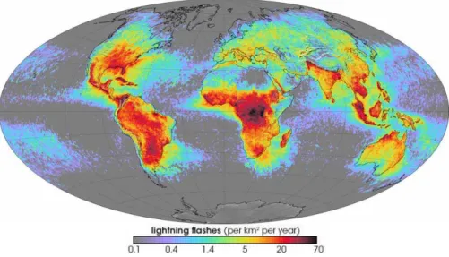
Lightning occurs mainly over land areas (see Fig. 9), with an average land/ocean ratio of about 6 to 10. (The precise ratio depends on the satellite used, on the resolution of the land mask, and on how coastal areas are assigned to land or ocean). Approximately 77% of all lightning occurs be-tween 30◦S and 30◦N, see Fig. 10. The flash rate is a max-imum over the Congo basin with annual mean flash den-sity of 80 km−2a−1. Over Brazil and Florida the density reaches 30 km−2a−1, and over Northern Italy, for compar-ison, it stays below 10 flashes km−2a−1 (Christian et al., 2003). For Germany, a value of 2.8 km−2a−1(mainly CG) has been reported based on a ground-based lightning loca-tion system (Finke and Hauf, 1996). In the tropics, regions with lightning activity may extend over several thousands of kilometres (Nickolaenko et al., 2006). Globally, most flashes
Table 8. Lightning flash rate (total, cloud-to-ground, and stroke rate). Flash rate
(s−1)
CG flash rate Stroke rate
Method Reference
100 – – Estimate assuming 1800
ac-tive thunderstorms, each lasting 1 h and causing 200 flashes
Brooks (1925); Mackerras et al. (1998)
400 100 1600 Review and extrapolations
based on the energy dissi-pated by lightning
Chameides et al. (1977); Chameides (1979a)
123±60 – – Photographs from two
DMSP satellites at dusk
Orville and Spencer (1979)
300 60 – Review Kowalczyk and Bauer (1981)
80±40 – – Photodetector on a DMSP
satellite recording lightning at dawn and dusk
Turman and Edgar (1982)
63±30 – – High-frequency radio
re-ceivers on the Japanese Ionosphere Sounding Satel-lite (ISS-b) satelSatel-lite
Kotaki and Katoh (1983)
65 10–14 – Combining DMSP, ISS-b,
ground-based observations, and a model
Mackerras et al. (1998)
44±5 – – from OTD data and a
continuous nine-year record of global lightning activity from LIS and OTD
Christian et al. (2003); Christian and Petersen (2005)
occur during the Northern Hemisphere summer (about 1.2 times more than in winter, because of larger land fraction in the Northern Hemisphere). There is a distinct seasonal and diurnal cycle. Over land, with the daily cycles of thun-derstorm convection, lightning peaks clearly in the afternoon hours between 14 and 18 local time, while being less vari-able over oceans (Hendon and Woddberry, 1993; Finke and Hauf, 1996; Williams et al., 2000; Dai, 2001; Ricciardulli and Sardeshmukh, 2002; Soriano et al., 2006); minimum of lightning activity occurs in the morning, at 6–8 local time (Nickolaenko et al., 2006), see Fig. 11.
Lightning activity increases dramatically with the depth and the vigour of convection (in particular updraft velocity) which is particularly pronounced over the tropical continents (Williams, 1985; Zipser et al., 2006). Lhermitte and Krehbiel (1979) using a network of three Doppler radars and ground-based lightning detection systems demonstrated that the total lightning flash rate correlates with in-cloud updraft velocity. Lightning is absent or highly unlikely if the updraft speed does not exceed a threshold of roughly 6–7 m s−1(mean) or 10–12 m s−1(peak), regardless of cloud depth (Zipser, 1994; Zipser and Lutz, 1994). Case studies show that the strongest
10% of convective updraft cores (including those in most of the intense hurricanes) have average vertical velocities ex-ceeding 4–5 m s−1 over oceans, compared to 12–13 m s−1 over land (Jorgenson and LeMone, 1989; Lucas et al., 1994b; Williams and Stanfill, 2002; Anderson et al., 2005). Cer-tain supercell and multicell storms over land reach updraft velocities up to about 80 m s−1 (Cotton and Anthes, 1989; Lang et al., 2004; Mullendore et al., 2005; Chaboureau et al., 2007). Some ground-based radar and lightning observa-tions indicate that the flash frequency increases with cloud top height (Williams, 1985, 2001). However, even for the same cloud top brightness temperature, size and radar reflec-tivity, satellite data indicate that storms over water produce less lightning than comparable storms over land (Cecil et al., 2005).
The higher flash ratio over land is explained by more in-tense convection (“thermal hypothesis”) (Williams, 2005). Most oceanic storms have updrafts which are too weak to induce sufficiently ice and supercooled water for electrifi-cation (Zipser, 1994; Toracinta et al., 2002). The amount of convective available potential energy (CAPE) is similar over land and oceans. However oceanic updrafts achieve a
Table 9. Intra-cloud/cloud-to-ground flash number ratio.
IC/CG flash number ratio Method Author
3.35 (2–6) Satellite and ground observations. The
bracket lists the possible range of values.
Prentice and MacKerras (1977)
5 Review Kowalczyk and Bauer (1981)
3.6–4 Satellite and ground observations Proctor (1991)
2.3 Ground-based lightning observations Mackerras and Darvenzina (1994)
4 Review Price et al. (1997b)
4.4± 1 Satellite and ground observations Mackerras et al. (1998)
2.8±1.4 (1–9) OTD and NLDN data over the
continen-tal USA. The bracket lists extreme mean values at various stations.
Boccippio et al. (2001)
2±0.6 (0.75–7.7) Data from OTD, LIS, and ground-based
lightning detection instruments denoted CIGRE-500 and CGR3, over Australia. The bracket lists extreme mean values at various stations.
Kuleshov et al. (2006)
3.5 (0–12) Data from OTD and a ground-based
light-ning detection network over Spain. The bracket lists the spatial variability of the mean values over the Iberian peninsula.
Soriano and de Pablo (2007)
lower fraction of their potentially available updraft velocities because of higher water loading (reducing buoyancy), more lateral entrainment, less buoyancy at low levels (Lucas et al., 1994a), and lower cloud base (Lucas et al., 1994b; Mushtak et al., 2005; Williams et al., 2005). The higher cloud base over land correlates with larger scales in the boundary layer, wider updrafts, less entrainment, and larger ice content above the freezing level (Lucas et al., 1994b; Zipser and Lutz, 1994; Williams and Stanfill, 2002).
Differing aerosol concentrations have also been proposed as a factor on the observed land-ocean contrasts (“aerosol hypothesis”) (Takahashi, 1984; Molini´e and Pontikis, 1995; Rosenfeld and Lensky, 1998; Steiger et al., 2002; Williams et al., 2002; Andreae et al., 2004). Wet land regions, like the Amazon basin in the wet season, act like a “green ocean” with reduced lightning activity (Williams et al., 2002). The presumed role of increased aerosol concentration is a reduced mean droplet size, narrower cloud droplet spectra, deeper mixed phase region in the cloud, additional charge separation in this region, enhanced lightning downwind of the aerosol source, and reduced particle sizes of ice crystals (Lyons et al., 1998a; Sherwood et al., 2006). Aerosols also impact the electrical conductivity of the atmosphere (Rycroft et al., 2000). A microphysical model study shows that different boundary layer aerosol causes differences in cloud condensa-tion nuclei (CCN), which influences thunderstorm charging (Mitzeva et al., 2006). Recent experiments provide mixed
support for the idea that smoke aerosols may impact CG po-larity, and suggest a possible link between drought condi-tions and lightning properties instead (Lang and Rutledge, 2006). Sensitivity of lightning to natural ground radioactiv-ity (Rakov and Uman, 2003), and to cosmic rays and the solar cycle has been also considered (Rycroft et al., 2000; Williams, 2005), but such influences are difficult to detect (Harrison, 2006). An analysis of the annual number of thun-der days versus island area gives more support to the thermal than the aerosol hypothesis (Williams and Stanfill, 2002). Also the invariance of lightning activity for two months with high and low aerosol concentrations over the Amazon re-gion casts doubt on a primary role for the aerosol enhancing the electrification (Williams et al., 2002). Simply speaking, land lightning is dominant because land is hotter than ocean (Williams and Stanfill, 2002).
Observations of the strength or size of convective updrafts do not exist worldwide. Weather analysis data indicate the global distribution of intense storms (Brooks et al., 2003). Proxies for convective intensity are given by satellite data of minimum passive microwave brightness temperature (at 37 and 85 GHz), maximum vertical extent of radar reflectiv-ity values (e.g., 20 or 40 dBZ), and maximum radar reflec-tivity at some height level (e.g. >6.5 km). Such data are available from the TRMM satellite in the tropics. Global data are available from the 85-GHz passive microwave sen-sor on a Defence Meteorological Satellite Program (DMSP)
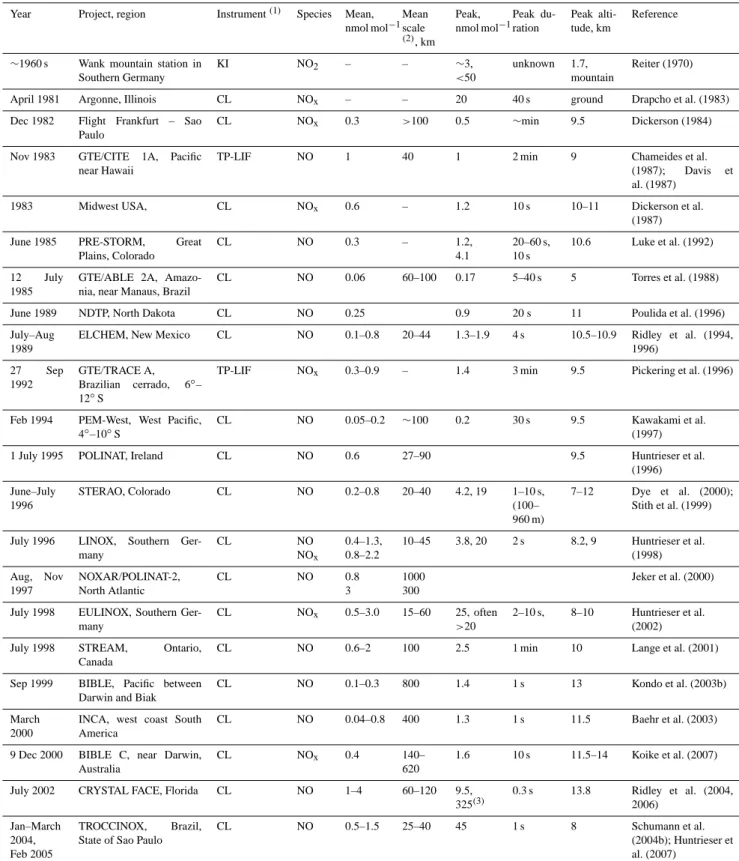
Table 10. Enhancements of NO and NOxmixing ratios measured in situ near thunderstorms.
Year Project, region Instrument(1) Species Mean,
nmol mol−1 Mean scale (2), km Peak, nmol mol−1 Peak du-ration Peak alti-tude, km Reference
∼1960 s Wank mountain station in Southern Germany KI NO2 – – ∼3, <50 unknown 1.7, mountain Reiter (1970)
April 1981 Argonne, Illinois CL NOx – – 20 40 s ground Drapcho et al. (1983) Dec 1982 Flight Frankfurt – Sao
Paulo
CL NOx 0.3 >100 0.5 ∼min 9.5 Dickerson (1984)
Nov 1983 GTE/CITE 1A, Pacific near Hawaii
TP-LIF NO 1 40 1 2 min 9 Chameides et al.
(1987); Davis et al. (1987)
1983 Midwest USA, CL NOx 0.6 – 1.2 10 s 10–11 Dickerson et al.
(1987) June 1985 PRE-STORM, Great
Plains, Colorado CL NO 0.3 – 1.2, 4.1 20–60 s, 10 s 10.6 Luke et al. (1992) 12 July 1985
GTE/ABLE 2A, Amazo-nia, near Manaus, Brazil
CL NO 0.06 60–100 0.17 5–40 s 5 Torres et al. (1988)
June 1989 NDTP, North Dakota CL NO 0.25 0.9 20 s 11 Poulida et al. (1996) July–Aug
1989
ELCHEM, New Mexico CL NO 0.1–0.8 20–44 1.3–1.9 4 s 10.5–10.9 Ridley et al. (1994, 1996) 27 Sep 1992 GTE/TRACE A, Brazilian cerrado, 6◦– 12◦S
TP-LIF NOx 0.3–0.9 – 1.4 3 min 9.5 Pickering et al. (1996)
Feb 1994 PEM-West, West Pacific, 4◦–10◦S
CL NO 0.05–0.2 ∼100 0.2 30 s 9.5 Kawakami et al. (1997)
1 July 1995 POLINAT, Ireland CL NO 0.6 27–90 9.5 Huntrieser et al.
(1996) June–July 1996 STERAO, Colorado CL NO 0.2–0.8 20–40 4.2, 19 1–10 s, (100– 960 m) 7–12 Dye et al. (2000); Stith et al. (1999)
July 1996 LINOX, Southern Ger-many CL NO NOx 0.4–1.3, 0.8–2.2 10–45 3.8, 20 2 s 8.2, 9 Huntrieser et al. (1998) Aug, Nov 1997 NOXAR/POLINAT-2, North Atlantic CL NO 0.8 3 1000 300 Jeker et al. (2000)
July 1998 EULINOX, Southern Ger-many
CL NOx 0.5–3.0 15–60 25, often
>20
2–10 s, 8–10 Huntrieser et al. (2002) July 1998 STREAM, Ontario,
Canada
CL NO 0.6–2 100 2.5 1 min 10 Lange et al. (2001)
Sep 1999 BIBLE, Pacific between Darwin and Biak
CL NO 0.1–0.3 800 1.4 1 s 13 Kondo et al. (2003b)
March 2000
INCA, west coast South America
CL NO 0.04–0.8 400 1.3 1 s 11.5 Baehr et al. (2003)
9 Dec 2000 BIBLE C, near Darwin, Australia
CL NOx 0.4 140–
620
1.6 10 s 11.5–14 Koike et al. (2007)
July 2002 CRYSTAL FACE, Florida CL NO 1–4 60–120 9.5, 325(3) 0.3 s 13.8 Ridley et al. (2004, 2006) Jan–March 2004, Feb 2005 TROCCINOX, Brazil, State of Sao Paulo
CL NO 0.5–1.5 25–40 45 1 s 8 Schumann et al.
(2004b); Huntrieser et al. (2007)
(1)CL: Chemiluminescence from the reaction of NO+O
3; KI: Method on the basis of a chemical reaction between NO2gas and a diluted KI
solution; TP-LIF: two-photon laser-induced fluorescence. (2) Horizontal mean scale of mean NO or NO
x enhancements; -: no information available; if only one value is given, the information
available is insufficient (or has not yet been evaluated in detail) to specify a range.