HAL Id: hal-02867990
https://hal.archives-ouvertes.fr/hal-02867990
Preprint submitted on 16 Jun 2020
HAL is a multi-disciplinary open access
archive for the deposit and dissemination of
sci-entific research documents, whether they are
pub-lished or not. The documents may come from
teaching and research institutions in France or
L’archive ouverte pluridisciplinaire HAL, est
destinée au dépôt et à la diffusion de documents
scientifiques de niveau recherche, publiés ou non,
émanant des établissements d’enseignement et de
recherche français ou étrangers, des laboratoires
Redundancy of hyperbolic triangle groups in spherical
CR representations
Raphaël Alexandre
To cite this version:
Raphaël Alexandre. Redundancy of hyperbolic triangle groups in spherical CR representations. 2020.
�hal-02867990�
Redundancy of hyperbolic triangle groups in
spherical CR representations
Raphaël V. A
LEXANDRE*June 16, 2020
Abstract
Falbel, Koseleff and Rouillier computed a large number of boundary unipotent CR representations. Those representations are not always discrete. By experimen-tally computing their limit set, one can determine that those with fractal limit sets are discrete. Most of those discrete representations can be classified into (3, 3, n) complex hyperbolic triangle groups. By exact computations, we verify the existence of those triangle representations, which have unipotent boundary holonomy. We also show that many representations are redundant: for n fixed, all the (3, 3, n) representations encountered are conjugated and only one among them is uniformizable.
Contents
1 Introduction 2
2 Elements of complex hyperbolic geometry 5
2.1 Limit sets . . . 6
2.2 Complex hyperbolic triangle groups . . . 6
3 Experimental approach 9 3.1 Computing limit sets . . . 10
3.2 Complex hyperbolic (3, 3, n) triangle groups . . . . 10
4 Redundancy 11 4.1 (3, 3, 4) – m004, m022, m029, m034, m081 and m117 . . . 17 4.2 (3, 3, 5) – m009, m015, m142 and m146 . . . 19 4.3 (3, 3, 6) – m023 . . . 19 4.4 (3, 3, 7) – m032, m045 and m039 . . . 20 4.5 (3, 3, ∞) – m129 and m203 . . . 21 *Institut de Mathématiques de Jussieu-Paris Rive Gauche, Sorbonne Université, 4 place Jussieu, 75252
Paris Cédex, France. ACG, OURAGAN (IMJ-PRG, INRIA Paris, Sorbonne Université, Université de Paris, CNRS). Email address:[email protected].
1 Introduction
We are interested in triangle groups Λ(p,q,r ) = ¿ a, b, c ; a 2 = b2= c2= e, (ab)p= (bc)q= (ca)r= e À (1) and how they can be represented into the Lie group PU(2, 1) by complex reflections, that is to say, with a, b and c all being complex reflections with respect to complex geodesic lines in the complex hyperbolic plane H2C. Such a representation is called a
complex hyperbolic triangle group, denoted by∆(p,q,r ), and the images of a, b and c
are often denoted by I1, I2and I3. An additional hypothesis is thatπp+πq+πr < π and
can be interpreted as the requirement for the triangle to lie in the hyperbolic plane. Triangle groups represented in PO(2, 1) (which is the transformation group of the
real hyperbolic plane) are fully prescribed by p, q and r (up to conjugation), whereas
in PU(2, 1) (which is the transformation group of the complex hyperbolic plane) an additional parameter controls the representation. This additional parameter can be interpreted as follows. One can always set two vertices of the triangle in a same real plane of H2C. The last vertex has to be placed at the intersection of the complex geodesic lines issued from the previous vertices. That intersection is a one-dimensional topological space and it represents the possible values of the additional parameter. Only one of those values corresponds to the case where the last vertex lies in the same previous real plane (and therefore corresponds to a R-Fuchsian representation). This parameter is called the angular invariant.
Complex hyperbolic triangle groups are a very rich class of representations in PU(2, 1) and one can ask whether it covers many known representations. In par-ticular, a large number of fundamental groups’ representations of knots’ and links’ complements are known in PU(2, 1). Falbel, Koseleff and Rouillier [FKR15] explic-itly computed those representations with unipotent boundary for complements described by four or less tetrahedra. The additional hypothesis of unipotent bound-ary is strong but allows this explicit computation that remains a highly complex numerical problem.
Those representations are accompanied by some delicate questions. Which
representations are discrete? Which are complex hyperbolic triangle groups?
In the early stages of those researches, Falbel [Fal08] constructed the unipotent boundary representations of the figure-eight knot. Those (essentially) three represen-tations have two discrete represenrepresen-tations among them, which are indeed complex hyperbolic triangle groups. To be more specific, those two representations can be identified with the even-length words’ normal subgroup of a complex hyperbolic triangle group∆(3,3,4).
When complex hyperbolic triangle groups were exposed by Schwartz [Sch02] in an ICM talk, he proposed the following conjecture which allows to compare the previous two emphasized questions: if we find a complex hyperbolic triangle group, is it a discrete and injective representation?
Conjecture 1.1 (Schwartz). A complex hyperbolic triangle group∆(p,q,r ) is a discrete and injective representation, if and only if I2I3I1I3and I1I2I3are both not elliptic.
Note that, in some rare cases, I2I3I1I3and I1I2I3 can have finite order and
Thompson [Tho10] showed that there exists a representation∆(3,3,4) with I2I3I1I3
of order 7 and a representation∆(3,3,5) with I2I3I1I3of order 5, and that both
repre-sentations are lattices.
A first step toward this conjecture is a result of Grossi [Gro07]. It shows that in the case of (p, q, r ) = (3,3,n), the fact that I2I3I1I3is not elliptic implies that I1I2I3is
not either. A proof of Schwartz’ conjecture in the case of (3, 3, n) has been given by Parker, Wang and Xie [PWX16] and the case of (3, 3, ∞) has been studied by Parker and Will [PW17].
Theorem 1.2 ([PWX16],[PW17]). Let 4 ≤ n ≤ ∞. Let Γ be a hyperbolic (3,3,n) triangle group. ThenΓ is a discrete and faithful representation of ∆(3,3,n) if and only if I2I3I1I3 is not elliptic.
This allows the following study: takeρ a boundary unipotent representation; is it discrete? Is it triangular? Both questions are here treated in a systematic and experimental manner.
To study the discreteness of a representation we chose to experimentally compute its limit set. This set is an attractor for the iteration dynamic and a simple argument allows to prove the discreteness: if this limit set is fractal then the representation is discrete (unfortunately, the converse does not hold).
Those representations with fractal limit sets are then set aside from the others. There are only two dozens of them (in comparaison of hundreds). They are then manipulated in order to try to prove that they come from a complex hyperbolic triangle group. We show that many of them are in fact triangle groups with (p, q, r ) = (3, 3, n) with n ≥ 4.
Since those representations are discrete, I2I3I1I3is not elliptic. In our examples,
we show that it is even parabolic unipotent and that the conjugacy class can be chosen so that I2I3I1I3generates the boundary holonomy of the fundamental group.
We would like to stress this last phenomenon. When a manifold M has an abstract triangle representationρ : π1(M ) → Λ(p, q,r ), then this representation has various
embeddingsπ1(M ) → Λ(p, q,r ) → ∆(p, q,r ) ⊂ PU(2,1) by the choice of the angular
in-variant. Only one representation∆(p,q,r ) is such that I2I3I1I3is parabolic unipotent.
In every example that the author encountered, this choice implied that the boundary holonomy is also parabolic unipotent and even described by the element I2I3I1I3. If
this phenomenon was always true, it would justify the search for triangle representa-tions using only the computation of boundary unipotent CR representarepresenta-tions. It is a drastic reduction. For example, the figure-eight knot has a two-dimensional charac-ter variety [Fal+16] but only three (up to complex conjugation) different unipotent boundary representations.
A phenomenon that will also interest us here is redundancy: among all the (3, 3, n) triangle groups’ representations (with n fixed) appearing in the census in [FKR15], only one corresponds to a uniformization of the underlying CR structure.
There is a delicate relationship between a CR representation of a manifold M and a uniformizable CR representation of M . In the latter case, the image groupΓ completely determines M : if U is its discontinuity domain then U /Γ is diffeomorphic to M (that is the definition of being uniformizable). Interestingly, it is very hard to determine whether a CR representation is uniformizable. The algebraic compu-tations of the CR represencompu-tations do not involve a conservation of the topological information.
Deraux [Der15] first showed that m009 and m015 are two manifolds with bound-ary unipotent CR representations∆(3,3,5) which are conjugated, but only the repre-sentation of m009 is uniformizable. In fact, once we know that two reprerepre-sentations are conjugated, then it follows that only one of them can be uniformizable by an evident topological argument.
The final result of the present work is:
Theorem(4.1). In the following table, the manifolds have a (3, 3, n) complex hyperbolic
triangle group representation, with the normal subgroup of the even-length words for image. Furthermore, all those representations (for a shared a column) are the same, up to conjugation and complex conjugation. The starred manifolds correspond to the uniformizable representations. ∆(3,3,4) ∆(3,3,5) ∆(3,3,6) ∆(3,3,7) ∆(3,3,∞) m004* m009* m023* (m039)* m129* m022 m015 m032 m203 m029 m142 m045 m034 m146 m081 m117
The even-length subgroups of the triangle groups∆(3,3,n) with I2I3I1I3parabolic
unipotent were finely studied by a theorem of Acosta. This theorem allows to identify the manifold at infinity and to check which manifolds have a uniformizable triangle representation.
Theorem 1.3 ([Aco19]). Let 4 ≤ n ≤ ∞. Let Γ be a hyperbolic (3,3,n) triangle group. Suppose that I2I3I1I3is parabolic unipotent. LetΓ0⊂ Γ be the subgroup of even-length words. Then the manifold at infinity of H2C/Γ0is the Dehn surgery with slope (1, n − 3) on any cusp of the Whitehead link complement.
In section 2, we succinctly expose a few elements of complex hyperbolic geometry that are necessary to the subject. In section 3, we explain how the numerical experi-ments were driven. We also propose visual clues in order to recognize the limit sets of the various triangle representations∆(3,3,n) with n varying and I2I3I1I3always
parabolic unipotent. Finally, in section 4 we summarized the various representa-tions with an apparent fractal limit set. We show that a subclass is only composed of∆(3,3,n) triangle groups. For this, we only employ formal computations, so the result is certain. We also explain how to retrieve which of each class for n fixed is uniformizable.
Note This paper is part of the author’s thesis, in progress under the supervision of
Elisha Falbel.
Acknowledgments The author enjoyed many and very fruitful conversations. First
of all, of course, I am very thankful to Elisha Falbel. This work could not have been executed without him. Since the early stages in making the experimental tools, Fab-rice Rouillier and Antonin Guilloux have been of precious help for the improvement of my code and its expanding. Across countries, Mathias Görner has been essen-tial to me in order to correctly use the tools provided by SnapPy. Without them, it
is clear that many efforts would not have been made to make the program faster, clearer and easier to use in a larger context. The code is open-source and accessible from the webpage of the author. I would also like to thank Pierre Will for taking the precious time to help me understand elementary aspects of the theory of complex hyperbolic groups. Finally, I have been pleased to exchange with Miguel Acosta. His understanding of both experimental and theoretical aspects has been very precious to me.
2 Elements of complex hyperbolic geometry
In this first section, we expose the main tools and notions in use. One can compare with [Wil16], [Gol99], [Pra05] and [CG74].
We consider the space C2,1, that is to say C3equipped with the Hermitian product
〈z, w〉 = z1w1+ z2w2− z3w3. (2)
The linear subspace of the vectors verifying 〈z, z〉 < 0 can be projectivised in CP2and is identified to the complex hyperbolic plane, H2C. In the affine chart z3= 1, one can
identify H2Cwith the set of vectors verifying |z1|2+ |z2|2< 1. This description of the
complex hyperbolic plane is also known as the Klein model of H2C. Its boundary in the complex projective plane is a differentiable sphere S3and is given by |z1|2+ |z2|2= 1.
Those points are in correspondance with the non-null vector lines in C2,1verifying 〈z, z〉 = 0.
The orthogonal group of C2,1is U(2, 1) and its projectivised version is PU(2, 1). To-gether with the complex conjugation, the group áPU(2, 1) is the transformation group of H2Cand also of its boundary sphere. This last geometrical structure ( áPU(2, 1), S3) is the spherical CR structure and (PU(2, 1), S3) is the orientation-preserving spherical CR
structure.
Let A ∈ SU(2,1). If A has a fixed point in H2Cthen A is elliptic. If inf{d (x, A(x))} > 0 with d the associated distance function of H2Cthen A is loxodromic (or hyperbolic). Otherwise, A is parabolic. One can determine the type of A by looking at its trace. We follow Goldman [Gol99] and let
f (τ) = |τ|4− 8Re(τ3) + 18|τ|2− 27. (3) If f (tr A) > 0 then A is loxodromic, if f (tr A) < 0 then A is elliptic (in fact regular elliptic: all its eigenvalues are different). When f (tr A) = 0 there are three cases: if tr(A)3= 27 then A is parabolic unipotent (all its eigenvalues are 1), otherwise it is either elliptic (and therefore a reflection with respect to a point or a complex geodesic) or ellipto-parabolic (a screw transformation along a complex geodesic). Note that whenτ is real:
f (τ) = (τ + 1)(τ − 3)3, (4) and (under the hypothesis that tr(A) is real) A is therefore regular elliptic if tr(A) ∈ ] − 1,3[, is loxodromic if tr(A) 6∈ [−1,3] and is parabolic unipotent if tr(A) = 3.
Let M be a smooth manifold andπ1(M ) its fundamental group. A representation ρ : π1(M ) → PU(2,1) is a (CR) uniformization of M if U /ρ(π1(M )) is diffeomorphic to M , where U ⊂ ∂H2Cis the domain of discontinuity ofρ(π1(M )). Whenρ is discrete, U = ∂H2C− L(ρ(π1(M ))), where L(ρ(π1(M ))) is the limit set ofρ(π1(M )). The next
section will describe this set. A manifold admitting such a representation is said to be (CR) uniformizable. Those manifolds are of high matter in the study of spherical
CR structures and are determined by the algebraic data ofρ. In general, U/ρ(π1(M ))
is a smooth manifold but is too hard to identify. It remains unknown which three-manifolds are CR uniformizable.
2.1 Limit sets
LetΓ ⊂ PU(2,1) be a subgroup. Its limit set L(Γ) is given by:
L(Γ) = Γ · p ∩ ∂H2C, (5)
where p ∈ H2Cis any point (L(Γ) is independent of this choice).
Lemma 2.1. The main properties of this set are the following. (Compare with [CG74].) 1. The limit set L(Γ) is compact and Γ-invariant.
2. If A ⊂ ∂H2Cis compact,Γ-invariant and is constituted of at least two points, then A ⊂ L(Γ).
3. If L(Γ) = ; then Γ fixes a point in H2
C.
4. If L(Γ) has at most two points, then L(Γ) is said to be elementary, otherwise it has an infinity number of points and is perfect (each point is an accumulating point).
An important result is the following.
Proposition 2.2 ([CG74]). IfΓ is not discrete then L(Γ) is either elementary, or equal to∂H2C, or equal to the boundary of a totally geodesic proper subspace, that is to say a smooth circle.
By consequence, if L(Γ) is a fractal, then Γ is discrete. It is a powerful experimental way to check ifΓ is discrete, since no abstract systematic argument allows to know this.
The auto-similarity property of limit sets can be justified by the following.
Lemma 2.3. LetΓ be a discrete subgroup of L(Γ) and suppose that L(Γ) is not elemen-tary. Let a ∈ L(Γ) be any point and V be any open neighbhorhood of a. Then there existsγ1, . . . ,γn∈ Γ such that
L(Γ) = [γi· V ∩ L(Γ). (6)
Proof. Let W = ∂H2C−
SΓ · V . It is compact and Γ-invariant. By construction, W can not have more than one point. If W = {b} then Γ let b fixed and it follows that
L(Γ) must be elementary since it is discrete (this relies on an observation on the
corresponding Heisenberg transformation group). Therefore W = ; and it follows that L(Γ) ⊂ SΓ ·V . By compacity of L(Γ), only a finite number of γi· V are necessary.
2.2 Complex hyperbolic triangle groups
We will now describe more precisely the complex hyperbolic triangle groups ∆(p,q,r ) = ¿ I1, I2, I3; I12= I22= I32= e, (I1I2)p= (I2I3)q= (I3I1)r= e À ⊂ PU(2, 1), (7)
with I1, I2and I3all three being complex reflections. If p or q or r is infinite, then the
corresponding relation vanishes.
Let∆(p,q,r ) be a non-singular complex hyperbolic triangle group (the geodesic lines corresponding to the reflections are distinct), with 2 ≤ p ≤ q ≤ r ≤ ∞ and
π
p+πq+πr < π. Any such triangle group can be represented by a complex hyperbolic triangle in H2C⊂ CP2.
Let H1, H2and H3be the vectorial hyperplanes of C3covering the sides of the
triangle in CP2. Let L1, L2and L3be the dual complex lines of those hyperplanes
defined by 〈Hi, Li〉 = 0. The group ∆(p, q, r ) is fully described by them.
We only need to choose a base vector for each Liin order to retrieve those lines. Furthermore, note that such base vectors form a basis of C3since the triangle group is non-singular.
Let vkbe a base vector of Lk, then
Ik(x) = −x +2〈vk, x〉
〈vk, vk〉vk (8)
is a complex reflection (note that 〈vk, x〉 and not 〈x, vk〉 makes this transformation linear) and verifies Ik(hk) = −hkfor any hk∈ Hk. That is to say, in CP2, Ik(hk) ≡ hk. Therefore Ikindeed defines the reflection fixing Hk. Because 〈vk, vk〉 > 0, one can normalize vkso that 〈vk, vk〉 = 1.
The last free parameters are an angle zk∈ S1for each vk. One can set z1and then
modify z2and z3so that 〈v1, v2〉 and 〈v2, v3〉 are real and positive. In general, 〈v1, v3〉
is not real and this lack can be measured by arg(〈v1, v3〉). From an intrinsic point of
view, that is to say without choosing the zk’s, the default for the vertices to be in a same real plane can be measured by
θ = −arg(〈v1, v2〉〈v2, v3〉〈v3, v1〉). (9)
The value ofθ is also known under the name of the angular invariant.
Once 〈vi, vj〉 = ci jare known, it is easy to evaluate the matrices of I1, I2and I3in
the basis (v1, v2, v3). I1= 1 2c12 2c13 0 −1 0 0 0 −1 (10) I2= −1 0 0 2c21 1 2c23 0 0 −1 (11) I3= −1 0 0 0 −1 0 2c31 2c32 1 (12)
We still have to see how p, q, r andθ determine 〈vi, vj〉 = ci j. For the time being, we suppose r < ∞. In fact, the matrix given by the ci j’s is equal to:
H = 1 cosπp cosπreiθ cosπp 1 cosπq
cosπre−i θ cosπq 1
And this shows that the ci j’s fully determine p, q, r andθ in return. This matrix is an Hermitian form preserved by I1, I2and I3. The determinant of this matrix is given by
1 + 2cos(θ)cosπ pcos π qcos π r − cos µπ p ¶2 − cos µπ q ¶2 − cos ³π r ´2 . (14)
This determinant allows to decide when H has (2, 1) for signature. Since the trace of
H is 3, it implies that at least one eigenvalue is positive. Therefore, its determinant is
negative if and only if H has (2, 1) for signature. That is equivalent to:
cos(θ) <−1 + cos ³ π p ´2 + cos ³ π q ´2 + cos¡πr ¢2
2 cosπpcosπqcosπr . (15)
That must be the case since the original Hermitian form 〈·,·〉 has (2,1) for signature. If p = 2 then c12vanishes and one can make both c23and c13real. Therefore,
(2, q, r ) complex hyperbolic triangle groups are rigid.
We now justify the expression of H . Up to conjugation, we can suppose that
H1∩ H2is generated by (0, 0, 1). This implies that v1and v2are both of the form
(x, y, 0). Therefore, every ci jis given by v1iv1j+ vi2v2j since at least one of vior vjhas a vanishing third coordinate.
Therefore, geometrically speaking, ci j is the cosine of the angle in C2formed by the complex lines generated by the first two coordinates of vi and vj. It is the real part of ci jthat is equal to the cosine of the angle formed by the vectors given by the first two coordinates of viand vj(see [Gol99, p. 36]).
Note that c13is non real in general, but of course 〈v1, eiθv3〉 = e−i θ〈v1, v3〉 = e−i θc13is real. The angle formed by H1and H2is equal to πp since (I1I2)p= e. By
taking the duals v1and v2, we get c12= ± cosπp but we made c12positive therefore c12= cosπp. Likewise, c23= cosqπand e−i θc13= cosπr.
Finally, one can compute, with i 6= j 6= k:
tr(IiIjIkIj) = 16|ci jck j|2− 16Re(c12c23c31) + 4|ci k|2− 1, (16)
and note that in our conventions, we have Re(c12c23c31) = c12c23c13cosθ. It shows
that tr(IiIjIkIj) determines ±θ once (p, q,r ) is known. Since the complex conjuga-tion changesθ into −θ, we deduce from our discussion the following results. In the case where (p, q, r ) = (3,3,r ) we have in fact:
tr(IiIjIkIj) = 4cos ³π r ´2 − 4 cosπ r cosθ. (17) Proposition 2.4 ([Pra05]). Let 3 ≤ p ≤ q ≤ r < ∞ be such that πp +πq+πr < π. A
representation of the triangle group
∆(p,q,r ) = ¿ I1, I2, I3; I12= I22= I32= e, (I1I2)p= (I2I3)q= (I3I1)r= e À (18)
into PU(2, 1) is determined byθ = arg(〈v1, v2〉〈v2, v3〉〈v1, v3〉) up to conjugation. Up to conjugation and complex conjugation, it is determined by tr(IiIjIkIj), with i 6= j 6= k.
Furthermore,θ verifies cos(θ) <−1 + cos ³ π p ´2 + cos³πq´2+ cos¡π r ¢2
2 cosπpcosπqcosπr (19)
and reciprocally, this condition suffices to define a representation with that value ofθ.
The parameterθ can be taken in ]0,π] since the complex conjugation exchanges
θ and 2π − θ. The possible values of tr(IiIjIkIj) are constrained by the preceding condition. For example, when (p, q, r ) = (3,3,r ), we have
cosθ <− 1 2+ cos ¡π r ¢2 1 2cosπr =−1 + 2 cos ¡π r ¢2 cosπr . (20)
If we take a look at the trace of IiIjIkIj, its maximum is given for cosθ minimal (that is to say −1) and its minimum by the maximum of cosθ.
tr(IiIjIkIj) ≤ 4cosπ r ³ cosπ r + 1 ´ , (21) tr(IiIjIkIj) > 4cos ³π r ´2 − 4 cosπ r à −1 + 2cos¡πr¢2 cosπr ! = 4 µ 1 − cos ³π r ´2¶ > 0. (22) This computation shows that the range of values of tr(IiIjIkIj) is included in R+and
therefore, the range for which∆(p,q,r ) is discrete and injective is of the form [3,m], with m the maximum stated before. The value 3 is indeed reachable: the minimum value for r is 4, since we have to verifyπp+πq+πr < π, and the maximum value of 4(1 − cos(πr)2) is indeed reached when r is minimal. This value for r = 4 is 1.
One can compute the angular invariant required to have IiIjIkIjparabolic unipo-tent. It is given by:
cosθ = cosπ
r −
3
4 cosπr. (23)
When one or several of p, q and r are non finite, we can get similar results by replacing the undefined ci jwith cosh(li j/2), where li jis the distance between the two complex hyperbolic geodesics Hiand Hj. See [Pra05]. In particular, it is still true that cosθ is determined by tr(IiIjIkIj).
3 Experimental approach
In this section, we explain how we experimentally computed the limit sets of the representations appearing in the census of Falbel-Koseleff-Rouillier [FKR15]. We also propose a comparative experiment by simulating the limit sets associated to the (3, 3, n) triangle groups. It will allow us to propose visual clues in order to distinguish the different (3, 3, n) triangle groups’ fractals when I2I3I1I3is parabolic.
The source code of the simulations and most of their results are available on the author’s webpage. The code has been made open-source.
3.1 Computing limit sets
Lemma 3.1. LetΓ ⊂ PU(n,1) be a subgroup. Let ΓLdenote the subgroup of the loxo-dromic elements. Suppose that the limit set L(Γ) is non elementary and that ΓL6= ;. Then the closure of the accumulation points’ set for the loxodromic iteration dynamic,
©x |∃g ∈ ΓL, lim gnx
0= xª , x0∈ H2C, (24)
is equal to the full limit set L(Γ).
Proof. This ensues from the following remark. Note that if g is loxodromic then
any conjugationγgγ−1is loxodromic too. Now,γx is equal to limγgnγ−1(x0). This
shows that the described set has two points (the attractive points of g and g−1) and is Γ-invariant.
It allows a first good strategy: computing attractive limit points of loxodromic elements. However, this strategy requires to compute a very large number of elements
g ∈ Γ. This can be done by generating words of length n. If Γ is described by two
generators, then there are approximately 3nwords of length n. An additional strategy consists in computing two lists of the half-length words and combining them at the last moment (in order to save a square root of memory space).
In practice, and this is particularly true with complex hyperbolic triangle groups, it is hard to get different points from such a computation. One can often see large concentrations of points in tiny boxes and even many copies of the same point. This is partly due to unknown relations between words, even at small length words.
Instead of only computing words and get their attractive limits, we used a second strategy in complement. When enough points are acquired, one can apply words on them (loxodromic or not) to get a better picture of the limit set. This method is much more efficient for it rarely makes redundant images. When nice symmetries are known (and for example, with complex hyperbolic triangles one knows the sym-metries I1, I2and I3), this allows a much better result. To symmetrize fully, one can
apply each symmetry successively on the set of points.
In practice, we first compute the attractive points of n1-length words, then apply
given symmetries on the set obtained, then apply n2-length words on them, and
again apply symmetries. At each step, we sort and select points in order to eliminate redundancy in the results.
At the end, we still have to project the points from CP2into R3⊂ ∂H2C. It can be done once a Hermitian form determining∂H2Cis known. We used a least-square method to solve the natural system of linear equations associated to such a Hermitian form in order to have this information.
3.2 Complex hyperbolic (3, 3, n) triangle groups
To compute the limit sets associated to PU(2, 1)-representations of (3, 3, n) triangle groups, we used our previous parametrization of the reflections I1, I2, and I3. We
already have all the tools necessary to ensure thatθ is acceptable and gives a discrete representation. Note that whenθ = π, it corresponds to a R-Fuchsian representation and the limit set is therefore a (R-)circle (since the representation preserves a real plane).
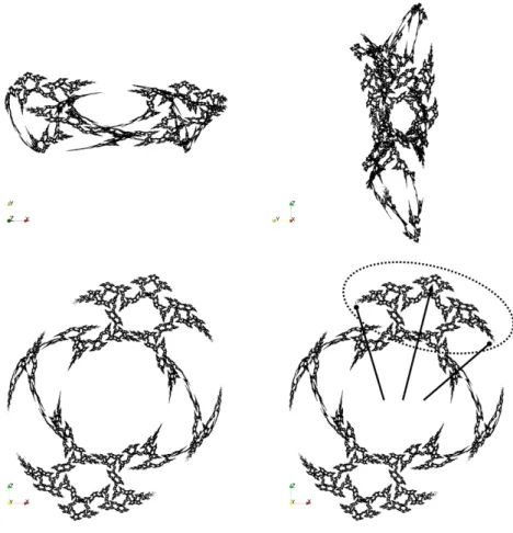
For n ∈ {4,5,6,7} we show three projections of the limit set and an additional diagram proposing a visual clue to recognize the limit set (figures 1, 2, 3, and 4). This
visual clue consists in looking for a pair of symmetric spikes and inspect the middle. We count the largest outer holes. When n = 4 there is none, when n = 5 there is one, when n = 6 there are two and when n = 7 there are three.
Figure 1: Hyperbolic triangle group (3, 3, 4) with I2I3I1I3parabolic.
The visual clues are pointed out in the following examples. See figures 5, 6, 7 and 8.
4 Redundancy
From the census of the unipotent boundary representations in [FKR15], we experi-mentally computed the limit sets. After a visual inspection, we kept the representa-tions that gave fractals.
Those representations come in pairs by complex conjugation of the coefficients. For each pair, we wrote down the identifier of one representation and of verified relations (they are true by exact computations) in the following table. Often, those relations allowed to reproduce the relation of the fundamental group. Each time, the fundamental group is presented by two generators and a relation.
Figure 2: Hyperbolic triangle group (3, 3, 5) with I2I3I1I3parabolic.
In the next table (table 1), we present all the representations which gave a fractal. Those accompanied by a star won’t be studied furthermore.
Additional remarks on the full experimental table It is already known that m004-1
and m004-3 are related by the composition of a figure-eight knot’s symmetry (see [Fal08]). It might be the same for m045-1 and m045-8 but this remains to be proved. The representation m038-1 presents the characteristics of a (3, 4, 4) complex hyperbolic triangle group. Indeed, m038 has such a representation according to a preprint of Ma and Xie that the author has been able to consult. The representation m137-5 presents the characteristics of a (3, 4, 5) complex hyperbolic triangle group.
The representations we selected all present characteristics of (3, 3, n) complex hyperbolic groups. We will indeed show this phenomenon.
Theorem 4.1. For each column of table 2, the manifolds have a (3, 3, n) complex hyperbolic triangle group representation, with the normal subgroup of the even-length words for image. Furthermore, all those representations (for a shared a column) are the same, up to conjugation and complex conjugation.
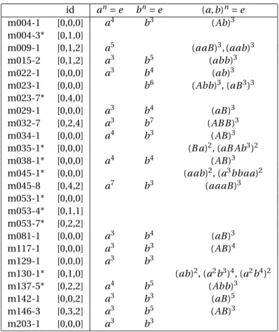
id an= e bn= e (a, b)n= e m004-1 [0,0,0] a4 b3 (Ab)3 m004-3* [0,1,0] m009-1 [0,1,2] a5 (aaB )3, (aab)3 m015-2 [0,1,2] a3 b5 (abb)3 m022-1 [0,0,0] a3 b4 (ab)3 m023-1 [0,0,0] b6 (Abb)3, (aB3)3 m023-7* [0,4,0] m029-1 [0,0,0] a3 b4 (aB )3 m032-7 [0,2,4] a3 b7 (AB B )3 m034-1 [0,0,0] a4 b3 (AB )3 m035-1* [0,0,0] (B a)2, (aB Ab3)2 m038-1* [0,0,0] a4 b4 (AB )3 m045-1* [0,0,0] (aab)2, (a3bbaa)2 m045-8 [0,4,2] a7 b3 (aaaB )3 m053-1* [0,0,0] m053-4* [0,1,1] m053-7* [0,2,2] m081-1 [0,0,0] a3 b4 (aB )3 m117-1 [0,0,0] a3 b3 (AB )4 m129-1 [0,0,0] a3 b3 m130-1* [0,1,0] (ab)2, (a2b3)4, (a2b4)2 m137-5* [0,2,2] a4 b5 (Abb)3 m142-1 [0,0,2] a3 b3 (aB )5 m146-3 [0,3,2] a3 b5 (AB )3 m203-1 [0,0,0] a3 b3
Table 1: Full experimental table.
∆(3,3,4) ∆(3,3,5) ∆(3,3,6) ∆(3,3,7) ∆(3,3,∞) m004* m009* m023* (m039)* m129* m022 m015 m032 m203 m029 m142 m045 m034 m146 m081 m117
Figure 3: Hyperbolic triangle group (3, 3, 6) with I2I3I1I3parabolic.
By consequence, for each column, at most one representation is a uniformization of the corresponding manifold. Deraux [Der15] encountered the same phenomenon with the manifolds m009 and m015. In fact, we can complete the picture with the following result of Acosta.
Theorem 4.2 ([Aco19]). Let 4 ≤ n ≤ ∞. Let Γ be a hyperbolic (3,3,n) triangle group. Suppose that I2I3I1I3is parabolic unipotent. LetΓ0⊂ Γ be the subgroup of even-length words. Then the manifold at infinity of H2C/Γ0is the Dehn surgery with slope (1, n − 3) on any cusp of the Whitehead link complement.
With SnapPy, it is possible to compute Dehn surgeries on the Whitehead link complement. Remember that m129 is the Whitehead link complement. In each column, we can identify a uniforming representation (which must be unique in the column). (In order to make SnapPy work correctly, one needs to call the manifold 521 and fill a cusp with the meridian equal to n − 3 and the longitude equal to 1.)
The manifolds in table 2 for which the corresponding (3, 3, n) representation is a uniformization were marked with a star. Those manifolds are: m004, m009, m023, m039 and m129. The first uniformization of m129 (the Whitehead link complement)
Figure 4: Hyperbolic triangle group (3, 3, 7) with I2I3I1I3parabolic.
was shown by Schwartz [Sch01], but the present uniformization by a (3, 3, ∞) triangle group with unipotent boundary was studied by Parker and Will [PW17].
About m039 This manifold is described with 5 tetrahedra and does therefore not
appear in the explicit census of [FKR15]. By the theorem of Acosta, it does have a rep-resentation with the even-length subgroup of the (3, 3, 7) complex hyperbolic triangle group having I2I3I1I3parabolic for image. We will construct this representation and
show that it has in fact parabolic unipotent boundary.
The same phenomenon happens for s000, the manifold obtained by Dehn surgery on the complement of the Whitehead link with the slope associated to the triangle group (3, 3, 8).
The method In the following subsections, corresponding to the different values
of n, we recognize the selected representations and reconstruct the triangle group representation in order to show the result with certainty. This is organized in three steps and for each one we give a table.
Figure 5: The representation m022-1 is of type (3, 3, 4).
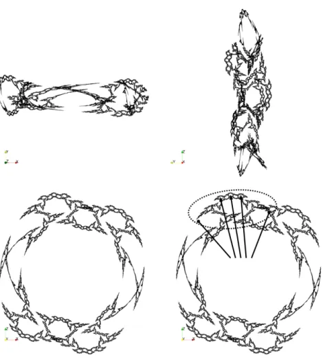
Figure 6: The representation m015-2 is of type (3, 3, 5).
1. The first table gives the informations from the census. That is to say, the way to retrieve the representation is the census (its identifier) and some relations (formally) verified that suggests the choice of the triangle group. Those relations always imply the fundamental group relation.
2. The second table gives a morphism from the fundamental group of the variety to the abstract triangle groupΛ(3,3,n). This is achieved by giving a presenta-tion of the fundamental group (that is always constituted of two generators and a relation) and the specification of the generators’ images. We check that the morphism chosen verifies the relations given in the preceding table and (there-fore) the fundamental group relation (showing that it is indeed a morphism). In this table, we also precise what the word corresponding to I2I3I1I3is. This
word can be experimentally computed with the representation of the census, and we can check that it is indeed parabolic unipotent (for one can take the trace once it is verified that the matrix is in SU(2, 1)).
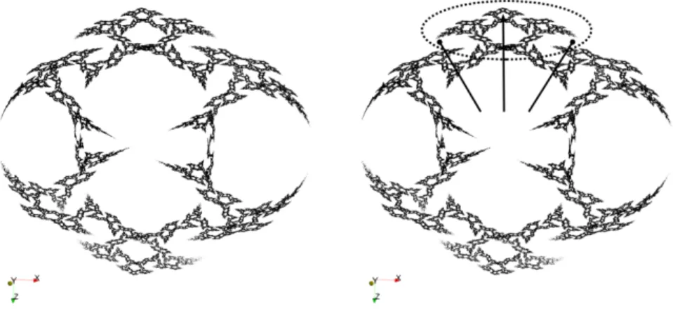
Figure 7: The representation m023-1 is of type (3, 3, 6).
Figure 8: The representation m032-7 is of type (3, 3, 7).
3. In the third table, we compute the peripheral holonomy. Equivalences of words are given according to the relations inscribed in the first table (that are verified by the abstract morphism previously constructed). This peripheral holonomy is computed in terms of I2I3I1I3. This implies that the abstract
representa-tion, once embedded in PU(2, 1) with the convenient angular invariant (that makes I2I3I1I3parabolic unipotent) must exist in the census. Therefore, this
constructed representation is indeed conjugated (or complex conjugated) to the one selected in the census, by unicity of the complex hyperbolic triangle group representations that has I2I3I1I3parabolic.
4.1 (3, 3, 4) – m004, m022, m029, m034, m081 and m117
The first table is computed with the help of the following code. i m p o r t s n a p p yi m p o r t n u m p y # D a t a s = ’ m 0 2 2 ’ i , j , k = 0 , 0 , 0 # M = s n a p p y . M a n i f o l d ( s ) G = M . f u n d a m e n t a l _ g r o u p () P = M . p t o l e m y _ v a r i e t y ( 3 ,’ all ’) . r e t r i e v e _ s o l u t i o n s ( p r e f e r _ r u r= True, v e r b o s e= F a l s e) S = [ [c o m p o n e n t for c o m p o n e n t in p e r _ o b s t r u c t i o n if c o m p o n e n t . d i m e n s i o n = = 0] for p e r _ o b s t r u c t i o n in P] K = S[i] [j] def f ( x ): m a t _ x = K . e v a l u a t e _ w o r d ( x , G ) r e t u r n [ [z . l i f t () for z in y] for y in m a t _ x] # S e a r c h t r i v i a l w o r d w o r d = ’ a ’ # to be c h a n g e d m a n u a l l y for i in r a n g e( 1 , 50 ): s = f ( w o r d*i ) if s = = [ [1 , 0 , 0], [0 , 1 , 0], [0 , 0 , 1] ] : p r i n t( i , s ) b r e a k id an= e bn= e (a, b)n= e m004-1 [0,0,0] a4 b3 (Ab)3 m022-1 [0,0,0] a3 b4 (ab)3 m029-1 [0,0,0] a3 b4 (aB )3 m034-1 [0,0,0] a4 b3 (AB )3 m081-1 [0,0,0] a3 b4 (aB )3 m117-1 [0,0,0] a3 b3 (AB )4
Here, we consider the abstract triangle group Λ(3,3,4) = ¿ I1, I2, I3; I12= I22= I32= e, (I1I2)3= (I2I3)3= (I3I1)4= e À . (25)
a b fundamental group’s relation I2I3I1I3= P
m004 I3I1 I3I2 aabABBAba B A m022 I3I2 I1I3 abbbbbabAAb Ab m029 I2I1 I3I1 aBabbbAAbbb aB B m034 I3I1 I1I2 aaabbABAbb B A A m081 I2I1 I3I1 abbbaBaaaaB aB B m117 I3I2 I3I1I2I3 aabbaabbABAbb aB
peripheral curves
m004 ab aB Ab AB ab ≡ (ab)3
P−1 P−3
m022 B a A Abab A ≡ B a
P−1 P−1
m029 abb ≡ aBB b A A Abbb ≡ e
P e m034 bbaa ≡ B A A A A AB B B A ≡ e P e m081 bba ≡ BB a B aaaB a ≡ BB a I1P−1I1 I1P−1I1 m117 b A B A A AB A ≡ b A P−1 P−1
4.2 (3, 3, 5) – m009, m015, m142 and m146
We iterate the same process.id an= e bn= e (a, b)n= e
m009-1 [0,1,2] a5 (aaB )3, (aab)3
m015-2 [0,1,2] a3 b5 (abb)3
m142-1 [0,0,2] a3 b3 (aB )5
m146-3 [0,3,2] a3 b5 (AB )3
This time, the triangle group is Λ(3,3,5) = ¿ I1, I2, I3; I2 1= I22= I32= e, (I1I2)3= (I2I3)3= (I3I1)5= e À . (26)
a b fundamental group’s relation I2I3I1I3= P
m009 I1I3 I3I1I3I1I3I2 aabABaaBAb B A m015 I2I1 I3I1I3I1 abbAAbbaBBB aB m142 I3I1I2I3 I2I3 abbaBabbaBaaaaB B A m146 I2I3 I3I1 aabbaaabbaaBAB aB peripheral curves m009 ab AB aaaB Ab ≡ (ab)2 P−1 P−1 m015 b A abb A A Abb ≡ (b A)−1 P−1 P m142 B A b A A Ab A ≡ B A P P m146 baa ≡ b A B AB AB B ≡ aB P−1 P
4.3 (3, 3, 6) – m023
id an= e bn= e (a, b)n= e m023-1 [0,0,0] b6 (Abb)3, (aB3)3The triangle group is ∆(3,3,6) = ¿ I1, I2, I3; I12= I22= I32= e, (I1I2)3= (I2I3)3= (I3I1)6= e À . (27)
a b fundamental group’s relation I2I3I1I3= P
m023 I3I1I3I1I3I2I3I1 I1I3 aBAbbABabbb B AB
peripheral curves
m023 bab bbaB AB abb ≡ (B AB)2
P−1 P2
4.4 (3, 3, 7) – m032, m045 and m039
id an= e bn= e (a, b)n= e
m032-7 [0,2,4] a3 b7 (AB B )3
m045-8 [0,4,2] a7 b3 (aaaB )3
The triangle group is Λ(3,3,7) = ¿ I1, I2, I3; I12= I22= I32= e, (I1I2)3= (I2I3)3= (I3I1)7= e À . (28)
a b fundamental group’s relation I2I3I1I3= P
m032 I1I2 I1I3I1I3I1I3 aaBBAbbbbbABB Abbb m045 I1I3I1I3 I2I1 aaabbaaaBAAAAB ba peripheral curves m032 B B B a bb A A Abba ≡ BBB a P−1 P−1 m045 AB b A A AB B B A A A ≡ ba P−1 P
We additionally construct a representation for m039 so that we complete our picture.
a b fundamental group’s relation
m039 I1I3 I3I1I3I1I2I1 aabABaaaaBAb
This representation verifies a7= (aab)3= (B aaaa)3and this implies the funda-mental group relation.
The peripheral holonomy is prescribed by U = AB and V = ab AB Abaaba. The
images are respectivelyρ(U) = 321313, ρ(V ) = 312132312123 (where we denoted
1, 2, 3 instead of I1, I2, I3). We can check thatρ(U) = ρ(V ) by computing ρ(U)−1ρ(V ).
Onceθ is fixed in order to have a triangle representation with I2I3I1I3parabolic
unipotent,ρ(V ) has its trace equal to 3 and this representation therefore has parabolic unipotent boundary.
4.5 (3, 3, ∞) – m129 and m203
id an= e bn= e (a, b)n= e
m129-1 [0,0,0] a3 b3
m203-1 [0,0,0] a3 b3
The triangle group is Λ(3,3,∞) = ¿ I1, I2, I3; I12= I22= I32= e, (I1I2)3= (I2I3)3= e À . (29)
This time, an additional parabolic unipotent element is given by I1I3.
a b fundamental group’s relation I2I3I1I3= P
m129 I3I1I2I3 I2I3 aaaBBabAAAbbAB B A m203 I3I1I2I3 I2I3 aaabbaaBAAABBAAb B A peripheral curves m129 A Ab ≡ ab A A Abb A ≡ B A P−1 P Ab b A A Aba ≡ B a (I3I2)I1I3(I3I2)−1 (I3I2)(I1I3)−1(I3I2)−1 m203 aab ≡ Ab B B A A AB ≡ e (I3I2)I1I3(I3I2)−1 e ab B A A AB B A A A ≡ e P−1 e
References
[Aco19] Miguel Acosta. “Spherical CR uniformization of Dehn surgeries of the
Whitehead link complement”. In: Geom. Topol. 23.5 (2019), pp. 2593–2664.
DOI:10.2140/gt.2019.23.2593.
[CG74] Shyan S. Chen and Leon Greenberg. “Hyperbolic spaces”. In:
Contribu-tions to analysis (a collection of papers dedicated to Lipman Bers) (1974),
pp. 49–87.
[Der15] Martin Deraux. “On spherical CR uniformization of 3-manifolds”. In: Exp.
Math. 24.3 (2015), pp. 355–370.DOI:10.1080/10586458.2014.996835. [Fal+16] E. Falbel et al. “Character varieties for SL(3,C): the figure eight knot”. In:
Exp. Math. 25.2 (2016), pp. 219–235.ISSN: 1058-6458.DOI:10 . 1080 / 10586458.2015.1068249.
[Fal08] Elisha Falbel. “A spherical CR structure on the complement of the figure eight knot with discrete holonomy”. In: J. Differential Geom. 79.1 (2008), pp. 69–110.ISSN: 0022-040X.
[FKR15] Elisha Falbel, Pierre-Vincent Koseleff, and Fabrice Rouillier. “Representa-tions of fundamental groups of 3-manifolds into PGL(3,C): exact compu-tations in low complexity”. In: Geom. Dedicata 177 (2015), pp. 229–255.
DOI:10.1007/s10711-014-9987-x.
[Gol99] William M. Goldman. Complex hyperbolic geometry. Oxford Mathematical
Monographs. The Clarendon Press, Oxford University Press, New York, 1999.
[Gro07] Carlos H. Grossi. “On the type of triangle groups”. In: Geom. Dedicata 130
(2007), pp. 137–148.DOI:10.1007/s10711-007-9209-x.
[Pra05] Anna Pratoussevitch. “Traces in complex hyperbolic triangle groups”. In:
Geom. Dedicata 111 (2005), pp. 159–185.DOI:10.1007/s10711- 004-1493-0.
[PW17] John R. Parker and Pierre Will. “A complex hyperbolic Riley slice”. In:
Geom. Topol. 21.6 (2017), pp. 3391–3451.DOI:10.2140/gt.2017.21. 3391.
[PWX16] John R. Parker, Jieyan Wang, and Baohua Xie. “Complex hyperbolic (3, 3, n) triangle groups”. In: Pacific J. Math. 280.2 (2016), pp. 433–453.DOI:10. 2140/pjm.2016.280.433.
[Sch01] Richard Evan Schwartz. “Degenerating the complex hyperbolic ideal
tri-angle groups”. In: Acta Math. 186.1 (2001), pp. 105–154.DOI:10.1007/ BF02392717.
[Sch02] Richard Evan Schwartz. “Complex hyperbolic triangle groups”. In:
Pro-ceedings of the International Congress of Mathematicians, Vol. II (Beijing, 2002). Higher Ed. Press, Beijing, 2002, pp. 339–349.
[Tho10] James M. Thompson. “Complex hyperbolic triangle groups”. PhD thesis.
Durham University, 2010.
[Wil16] Pierre Will. “Two-generator groups acting on the complex hyperbolic
plane”. In: Handbook of Teichmüller theory. Vol. VI. Vol. 27. IRMA Lect. Math. Theor. Phys. Eur. Math. Soc., Zürich, 2016, pp. 275–334.