Following food sources by artificial creatures in a virtual ecosystem

HAL Id: hal-03220761

https://hal.archives-ouvertes.fr/hal-03220761 Submitted on 10 May 2021

HAL is a multi-disciplinary open access archive for the deposit and dissemination of sci-entific research documents, whether they are pub-lished or not. The documents may come from teaching and research institutions in France or abroad, or from public or private research centers.

L’archive ouverte pluridisciplinaire HAL, est destinée au dépôt et à la diffusion de documents scientifiques de niveau recherche, publiés ou non, émanant des établissements d’enseignement et de recherche français ou étrangers, des laboratoires publics ou privés.

Nesrine Ouannes, Nouredinne Djedi, Yves Duthen, Hervé Luga

To cite this version:

Nesrine Ouannes, Nouredinne Djedi, Yves Duthen, Hervé Luga. Following food sources by artificial creatures in a virtual ecosystem. Stephan Bornhofen; Jean-Claude Heudin; Alain Lioret; Jean-Claude Torrel. Virtual words - Artificial Ecosystems and Digital Art Exploration, Science e-book, pp.99-116, 2012, 979-10-91245-06-7. �10.13140/RG.2.1.3502.1529�. �hal-03220761�

Following Food Sources by Artificial

Creatures in a Virtual Ecosystem

Nesrine Ouannes, Noureddine Djedi

LESIA Laboratory, Biskra University, Algeria

Yves Duthen, Hervé Luga

Institut de Recherche en Informatique de Toulouse Université de Toulouse 1, CNRS, Toulouse, France

Abstract

In this chapter a virtual ecosystem environment with basic physical law and energy concept has been proposed, this ecosystem is populated with 3D virtual creatures that are living in this environment in order to forage food. Artificial behaviors are developed in order to control artificial creatures. Initially, we study the behavior of herbivore’s creatures, which feed resources available in their environment. A genetic algorithm with an artificial neural network were implemented together to guarantee some of these behaviors like searching food. Foods are presented in different locations in the virtual ecosystem. The evolutionary process uses the physical properties of the virtual creatures and an external fitness function with several objectives that will conduct to the expected behaviors. The experiment evolving locomoting virtual creatures shows that these virtual creatures try to obtain at least one of the food sources presented in their trajectories. Our best-evolved creatures are able to reach multiple food sources during the simulation time.

1. Introduction

Researchers in Artificial life attempt to design and construct systems that exhibit the characteristic of living organisms. Among the great variety of biological systems that inspire and guide artificial life research, and according to Bedau (Bedau 2003) three broad areas can be identified according to the scale of their elementary: (a) At the microscopic scale, chemical, cellular and tissular systems; Wet ALife synthesizes living systems out of biochemical substances, (b) At the mesoscopic scale,

organismal and architecture systems; or the Soft ALife that uses simulations or other purely digital constructions that exhibit lifelike behavior, (c) At the macroscopic scale, collective and societal systems.

Our main objective is to inspire from nature and food chain process to create a virtual ecosystem. Developing artificial behaviors for artificial creatures in such ecosystems by hand is almost an impossible task (Reynolds 1994) that can be addressed by means of Evolutionary Algorithms.

Evolving behaviors of artificial creatures in three-dimensional, physical environments are subject of a variety of works; most of them are based on Karl Sims’ one (Sims 1994), (Sims (a) 1994).

Some of these models focus on developing morphologies and behaviors for artificial creatures (Miconi 2008), (Bongard 2010), (Lassabe 2007) and (Chaumont 2007).

Other models have attempted to study only the behaviors od artificial creatures such as those of Sims creatures; noting (Nakamura 2009) that examines how an artificial creature acquires adaptive swimming behaviors in an hydrodynamic environment, and (Nakamura 2009), (Iwadate 2009), (Pilat 2010) for light following task. Recent works have focused on studding foraging behaviors (Pilat 2012), (Chaumont 2011).

In some approaches, behaviors were studied in virtual ecosystems, like the ‘Avida’ system (Adami 1994) that is inspired from ‘Tierra’ system (Ray 1991), and the ‘LifeDrop’ system (Métivier 2002) comparable to ‘Gene Pool’ system (Ventrella 1998).

This chapter describes the first step made in the process of creating a complete ecosystem with artificial creatures that are simulated with 3-D shapes and with some physical properties. Artificial behaviors are developed in order to control artificial creatures. The artificial creatures living in the ecosystem are divided into four classes: producers (plants), 2 kinds of consumers (herbivores and carnivores) and decomposers such as bacteria. Initially, we study the behavior of herbivorous creatures, which feed on available resources in their environment.

In this part of our ecosystem, we present a controller model, which controls physically the simulated creatures in a biologically inspired manner: by evolving the neural connection weights of a neural network to obtain foraging behaviors. We model a virtual environment with a population of such creatures to study the evolution of some behaviors (walking, foraging) constrained by their energy consumption in a physically plausible 3D environment. The creatures must survive while maintaining their energy level that is computed according to their metabolism. The energy gained from eating decreases by a value depending on the cost of

motion. This metabolic model drives the creature to stabilize its consumption of energy and to reach more energy sources as possible during its lifetime.

The rest of this paper is organized as follows. We begin with describing the artificial creature model that is simulated using simple Newtonian physics. Then we will show how we adopt a recurrent neural network to control the creature's motions.

In the final section two experiments will be presented. In one only single food source was provided. In a more complex problem, a lot of food sources were present. We end with a discussion of the results obtained from the both experiments of evolved behaviors.

2. The Food-Following Model

2.1. Artificial Creature Model

We create the artificial creature by connecting rigid 3D body parts with joints and actuators. The kinematical model is then generated from, the geometrical data of the artificial creature (link lengths, type and position of joints etc.). We employ open dynamics engine (ODE1_{) as a simulation}

platform for the artificial creature. ODE is a free, industrial quality software library for simulating articulated rigid body dynamics. It is fast, flexible and robust, and it has built-in collision detection. Therefore, ODE is suitable for a realistic simulation of the physics of an entire creature.

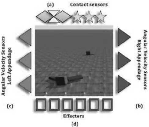
Figure 1 shows artificial creature model. This creature consists of three rectangular boxes jointed with two Ball and socket joints.

The artificial creature’s model presented in this paper is equipped with two food sensors. These two sensors are used as the only information about food sources.

We use recurrent neural network as controller that controls the motions of this artificial creature (locomotion). A genetic algorithm is then used to evolve more complex behaviors (following or looking for foods). Actuators are controlled by outputs of the network.

We use a physics-based model of an articulated creature that embodies the nonlinear relationships between the forces and the moments acting at each joint and the appendages etc., and the position, velocity and acceleration of each joint angle. In addition to the geometric data, a physically realistic model requires kinematic data and some physical properties as mass, gravity center and inertia matrix, for each link and joint, max/min motor torques and joint velocities which are difficult to simulate.

To simulate interaction with the environment detection and handling of collisions as well as suitable models of appendages-ground contacts are required. In the context of this simulation we use the open source Open Dynamics Engine (ODE) library that can handle collision detection for several geometric primitives.

Figure 1. A simple 3D Artificial Creature model used in our simulation, with a torso

and two appendages. This model has (a) two food sensors, a direction sensor and three contact sensors for each rigid body. The appendages have sensors attached to them, (b) three angular velocity sensors at the right one, and (c) three angular velocity sensors at the left one. It has also (d) six effectors.

2.2. Artificial Creature's Brain (The Controller)

An RNN is an artificial neural network (Heykin 1999) that is a well-known brain model. It consists of a set of neurons (units) and set of synapses (arcs) including self-coupling of individual neurons.

The artificial creature presented in this paper uses Elman (Elman 1990) Recurrent Neural Network for its biological plausibility and powerful memory capabilities.

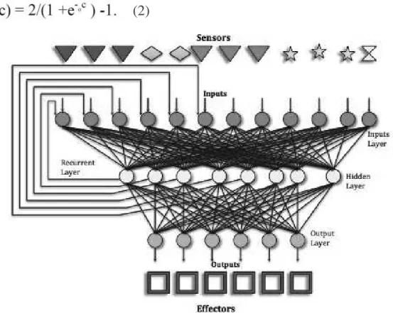
The topology of our network is made up of 4 layers: an input layer, a hidden layer, an output layer and a context layer. The number of neurons contained in the input and output layer depends on the artificial creature’s

morphology (i.e. the number of sensors and actuators). Each inter-neuron connection within the RNN is assigned a weight (see Figure 2).

The RNN network can operate either in discrete time as common in feed-forward networks, or in continuous time. In the latter case, using a simple neuron model, the dynamical behavior of the ith

node in the network is governed by the equation 1.

Where n is the number of neurons in the network, τ_i are time constants, γi is the output (activity) of node i, ωιj is the (synaptic) weight connecting

node j to node i, wij I

is the weight connecting input node j to node i, Ij is the

jth external input to node i, and bi is the bias term, which determines the

output of the neuron in the absence of inputs. σ() is a sigmoid function whose main purpose is to restrict the activity of the neurons to a given range. The hidden, context, and output layers of the RNN all use the same bipolar sigmoid activation function (see equation 2).

(2)

Figure 2. The Recurrent Neural Network Structure. It consists of four layers; input

(with 12 neurons), hidden (8 neurons), output (6 neurons) and context layer (6 neurons). There are arcs (inter-neuron connections with weights) and the Time response of this RNN is 5 Time Step.

2.3. Sensors and Actuators

The artificial creature uses a set of sensors to collect data from the environment and feeds it to the RNN. Sensors that monitor the internal state of the artificial creature, such as joint angles are referred to as proprioceptive sensors. In this setting, the current joint angles of the previous time step of the simulation are used by the evolved controller to compute the next set of motor signals for the artificial creature.

Simulating an artificial creature in a realistic environment most likely requires feedback loops between the artificial creatures control system and its body, as well as between the control system and the environment.

The set of external sensors link the creature to its environment. Those sensors can measure values such as the creature acceleration or till relative to a fixed coordinate frame, external forces applied to the bodies, etc. This artificial creature has:

- Two food sensors at the torso, those return the angle and the distance between the visible (in our experiments the creature's brain at time (t) sees only one food source) food source and themselves,

- Three contact sensors; one in each body part. The contact sensors indicate when a body makes contact with the ground plane;

- The Ball and socket joints contain angular velocity sensors that feed the rate of angular change back to the RNN.

- Finally, a direction sensor provides the ANN with a virtual compass. We control actuators sets implemented with the artificial creature that are three actuators in each appendage of the artificial creature. There are 12 sensors and 6 actuators in total.

In a control system, such as that used by the artificial creature, specifying the correct outputs for each possible input combination and state is practically impossible. In these situations, optimal behavior must be learned by exploration.

Genetic algorithms can be used as an optimization process to evolve neural network’s weights that prove to be robust solutions to difficult virtual-world learning tasks.

2.4. The Energy Flow

As mentioned earlier, we use in our experiments the energy consumption as one of the measures to select individuals in the evolution process, this concept is not used to found the threshold level to survive (which is realized with natural selection), but it is used to found the best creatures that can reach a lot of food sources by minimizing the loss of energy when they are walking.

Ei describes an artificial creature's energy content, all creatures in the virtual ecosystem have the same initial value at birth, the energy level is decreased every five Time Steps by a value that is defined by cost of motion. This value is measured by cumulated torques generated by actuators.

In order to increase the level of energy to avoid death, the artificial creature has to consume food sources that are placed in the virtual ecosystem. An artificial creature with energy equal to 0 dies (it stops motions because there is no more energy to use in its actuators) and after the expiration of its lifetime it will be removed from the population. Each food source provides with the same energy amount.

2.5. Chromosome

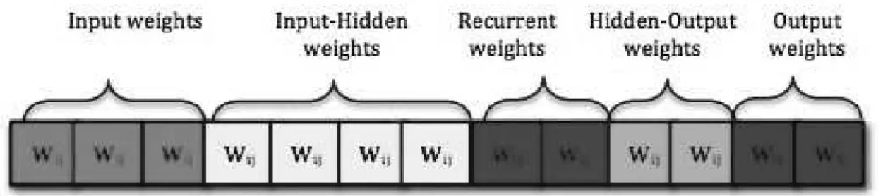
We use the Genetic Algorithm with a real number encoding. The GA optimizes weights of a neural network to acquire adaptive behaviors of the simulated artificial creature. The weights are stored within an artificial chromosome that can undergo different modifications (crossover and mutation). The figure 3 illustrates the chromosome structure.

Figure 3. The Chromosome Structure. This gene encodes a recurrent neural network weights, it has five regions, which present each one the interconnections between the four layers of the network. The weights encoded in this genome are organized like: input weights, input-hidden, recurrent, hidden-output and output weights.

The evolutionary algorithm is based on a population of 100 genotypes, which are randomly generated. This population of genotypes encodes the connection weights of 100 neural controllers. The evolutionary runs are performed using a fixed length genome that consists of 638 genes, with 1 gene per RNN weight. The number of connections in a neural network represents the number of genes in the chromosome; a floating-point number represents each gene.

3. Experimental Setup

We carry out experiments to examine how the simulated virtual creature can acquire following behaviors towards some food sources by walking towards them, and analyse the acquired walking behaviors.

The experimental environment is an open and continuous 3D space without obstacles. It is filled with two types of objects: virtual creatures and food sources. When a virtual creature moves towards a food source, its life energy is replenished by a certain amount. All food sources have the same size and the same amount of energy. A simple simulation screenshot is shown in the Color Plate 1.

This article describes two experimental setups:

(1) The case where one single food source is provided: where the fitness is given by measuring the energy level of an artificial creature and the distance travelled at the end of its lifetime.

(2) With more than one food source, a food source has a given maximum energy capacity which defines its initial energy content. If an artificial creature is in contact with a food source, a certain amount of energy is transferred from the source to the artificial creature and thereby consumed. The best creatures are those who have more energy quantities because after catching one food source they can go to catch another one until their lifetime is not expired.

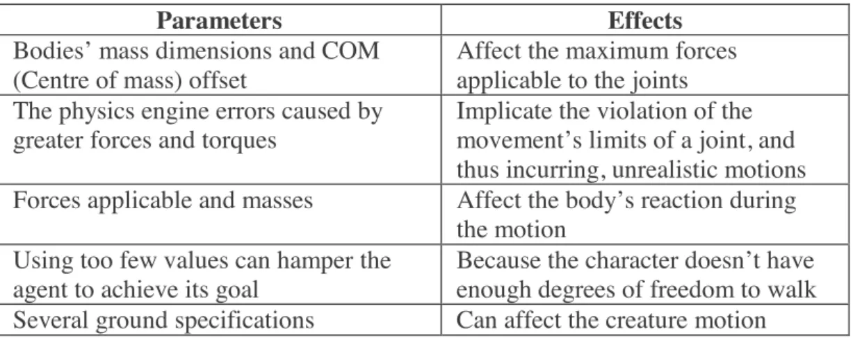
Table 1. Physics Parameters used by the Dynamic Engine.

Initially 100 creatures (individuals) are plunged in the simulator with one food source for each creature, in a first stage, after learning how to walk, the creature must evolve to reach the food source, secondary, we have setup an environment with a lot of food sources for each creature. Each creature catches its first food source (as in the first experiment) and it will update its sensory information in order to detect the next food source.

Parameters Effects

Bodies’ mass dimensions and COM (Centre of mass) offset

Affect the maximum forces applicable to the joints The physics engine errors caused by

greater forces and torques

Implicate the violation of the movement’s limits of a joint, and thus incurring, unrealistic motions Forces applicable and masses Affect the body’s reaction during

the motion Using too few values can hamper the

agent to achieve its goal

Because the character doesn’t have enough degrees of freedom to walk Several ground specifications Can affect the creature motion

The environment in which evolution occurs is extremely important to the final results. The simulated environment imposes similar constraints on the virtual creature as the natural environment would on a real creature of similar proportions. Different parameters have been used in our virtual creature’s model; the table 2 summarizes the effect of some parameters that are important to the generation of a realistic motion.

3.1. Evolution Setup

A population of 100 controller genomes is evolved through 1700 generations using a specific selection protocol combined with an elitist selection method. The rank between two creatures could be summarized as follow:

Begin

if (nbA>nbB) then A is selected; else

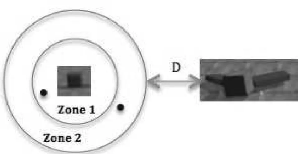
if (A in Zone 1) and (B in Zone 2) then A is selected;

else

if (A in Zone 2) and (B in Zone 1) then B is selected;

if (EA>EB)then A is selected; End.

Where nbA and nbB are the number of food sources consumed by the creature A and B, the Zone 1 is a circle about one meter from the food source seen by the creature and Zone 2 is about 2 meters. EA and EB are the energy level of each creature obtained in the end of the simulation.

The selection protocol is used to choice between two creatures A and B, this choice is based on three criteria: the firs one is when a creature has obtained more food sources, it will be chosen. If both creatures have not yet obtained food sources, so that the choice of the best creature will be based on distance traveled by each one, it is applied by testing the area (zone) where the creature exists at the end of the simulation (see figure 5), and the creature chosen is that existing in the closest area to the food source’s position (i.e. zone 1). The last criteria is applied when the two creatures are outside the two areas, in this case the choice of the creature will be based on its level of energy (i.e. the creature with the greatest amount of energy will be chosen).

Figure 5. Graphic explaining the selection protocol.

The genetic algorithm used here makes use of the standard single-point crossover operator at a rate of 70%. After the crossover operation, the gene has a probability of being mutated. The mutation operator uses a Gaussian perturbation rather than a uniform mutation.

3.1.1. The fitness function

To evaluate the fitness of an artificial creature, we test each artificial creature in the physics-based simulator for a constant simulation time (10 seconds for experiment 1 and 30 seconds for experiment 2) using the ANN coded by each chromosome. This function will be used to select individuals using both elite and tournament selection. In order to evaluate our controller’s global performance an aggregate function F is used, a multi-objective function that takes in consideration three fundamental points of evaluations which are scaled by the weights W1, W2 and W3 (see equation 1 in figure 3).

(3) Where:

- N is the maximization of the number of food sources obtained and consumed in 30 seconds;

- D is the minimization of the cumulated distance between the creature’s current place and the nearest food source during the artificial creature's motion (see equation 4);

- E is the minimization of the consumed energy, which is measured by cumulated torques generated by actuators (see equation 5).

F (in equation 3) is to maximize, D and E are also to minimize, it is why they are multiplied by (–). N∈ [0,3] minimum and maximum number

of food sources for each creature. D∈ [0,15] Zero is the start position, and 15 is the position of the third food source. Finally E∈ [0,1000] which is the interval of the energy amount.

To homogenize the interval of three variables N, D and E to the common interval {N, D, E}∈ [0,3000], we have chosen the weights values as: W1=1000, W2=200 and W3=3.

(4) (5)

Where T is the period of simulation, which is 1000 Time Steps in experiment 1 and 3000 in experiment 2 (10 and 30 seconds), Yf is the food source position and Yt is the position of the artificial creature at time t. A is the number of actuators in the artificial creature and Etj is the energy spent at each actuator.

The values obtained from these functions will be used to compare the individual’s performance between different generations and to generate statistical data.

4. Results and Discussion

The result motions of the artificial creatures that try to catch foods; look like walking behavior on the ground and they are obtained after more than 1700 generations. Some of these results are presented in the Movie of the evolved creatures2 _{where the artificial creatures in the latest generations walk faster}

than in the earliest ones.

The evolutionary process in this work was able to successfully produce a stable walking movement that allows the artificial creature to move towards their goals.

4.1. Following One Food Source

In first case where only single food source was provided, the artificial creature acquires effective motions to reach its goal as efficiently as possible.

Figure 6 shows some actuators outputs of the left and right normalizes appendages of the artificial creature during locomotion relative to a simulation period of 10 seconds. When the artificial creature moves like walking on the ground, actuators generate phases with different level values

between the left and the right joints but both joints advance with a symmetrical way; one time on the positive direction and other on the negative one and with pushing the torso which is always in contact with the ground.

Figure 6. The Output Actuator of the artificial creature.

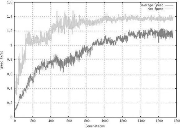
Figure 7 shows the speed values of locomotion realized by the evolved creatures. We note that the values of speed increase over generations, which means that the creatures walk faster, this allows them to catch a lot of food sources as possible and therefore, they recover energy that was lost during locomotion.

The energy level is inversely decreases than the speed, as presented in the figure 8, that shows the energy level decreasing over generations, except for the case where a creature grabs its food source, and that the amount of energy from this food source will be transferred to the creature.

Figure 9 shows the best and the average distances calculated by the artificial creature on walking toward the food source. The distance graph looks like a straight that decrease over generations, thing that means that the creature is nearing its food source, in generation 800 the distance value is close to zero (i.e. the artificial creature’s current place is equal to the food source position).

To better present the results obtained from the behavior of foraging food sources, we add another type of results representation, which is the shown in.

Figure 7. The Speed Graph performed by the artificial creatures during locomotion

over generations.

Figure 9. The Distance Graph realized by the artificial creature over generations.

Figure 10. Food Following Paths realized by the best (red lines) and the worst

Figure 10 shows the path of positions initiated by the creature heading towards its first food source; realized in 10 seconds of simulation (i.e. the first experiment).

4.2. Following More than One Food Source

The main goal of this work is to find with artificial evolution a foraging (or food following) behavior, that is important to the construction of an artificial ecosystem, for this reason, we setup a second experiment for the same behavior but with several food sources. Figure 11 summarizes the results obtained for this case.

Figure 11. The Distance graph for the best and the average of the population of

creatures that catch several food sources.

The evolutionary process in this experiment was able to successfully produce stable walking movements that allowed the virtual creature to move towards some food sources.

Our best-evolved creatures are able to reach multiple food sources during the simulation time as presented in the Distance Graph (see figure 11) where the values are decreased from 15 (i.e. distance travelled is zero) to a value that is close to zero (i.e. third source obtained).

5. Conclusion and future work

This chapter emphasizes on the first produced step towards the construction of a simulated virtual ecosystem. In this part we present experiments and some results of evolving artificial creature’s brain to obtain following behaviors.

All the obtained behaviors are the result of the artificial creature interacting with the environment via a simple sensory system. The resulting controllers are consistent with physical laws and provide motion, which are dominated by the Newtonian dynamics.

Our future studies will show the links between all the classes of our virtual ecosystem, which have to interact inside it. The next step we aim at is the study of a predator-prey model (with co-evolution of two populations). We will study the dynamics of a predator-prey system in a virtual ecosystem where the creatures have opposing goals as in (Miller 1994).

The third part will be to study decomposers behaviors; this task can be realized by modeling bacteria behaviors as in (Vlachosa 2005), in this study we propose a model that uses the artificial chemistry to simulate the bacterium chemotaxis and to use a chromosome that evolve and emerge more complex behaviors of bacteria. Finally the Plants growth is the fourth behavior to study which is a fascinate work to do. These classes (nodes) met together to form a food chain through the energy transfer.

References

Adami, C., Titus Brown, C., 1994. Evolutionary learning in the 2d artificial life system “avida”, Artificial Life IV, 3-37.

Auerbach, E., Bongard, J.C., 2010. Dynamic resolution in the coevolution of morphology and control, Artificial Life XII, H. Fellermann et al., 451-458. Bedau, M. A., 2003. Artificial life: Organization, adaptation and complexity from

the bottom up, Trends in Cognitive Sciences, 7(11), 505-512.

Chaumont, N., Egli, R., Adami, C., 2007. Evolving Virtual Creatures and Catapults,

Artificial Life XIII, The MIT Press, Cambridge, MA, 139-157.

Elman, Jeffrey L., 1990. Finding Structure in Time, Cognitive Science, 14, 179-211. Haykin., S., 1999. Neural Networks: A comprehensive foundation, Prentice Hall, 2nd

ed.

Holland, J., 1992. Adaptation in Natural and Artificial Systems, The MIT Press, Cambridge, MA.

Iwadate, I., Suzuki, I., Yamamoto, M., Furukawa, F., 2009. Evolving Amphibian Behavior in Complex Environment, ECAL 2009, G. Kampis, I. Karsai, E. Szathmáry (Eds.), Part I, LNCS 5777, Springer-Verlag, Berlin, 107-114. Lassabe, N., Luga, H., Duthen, Y., 2007. A New Step for Evolving Creatures,

Métivier, M., Lattaud, C., Heudin, J.C., 2002. A Stress-based Speciation Model in Lifedrop, Artificial Life VIII, The MIT Press, Cambridge, MA, 121-126. Miconi, T., 2008. In Silicon No One Can Hear You Scream: Evolving Fighting

Creatures, 11th European Conference on Genetic Programming, M. O'Neill, et al. (Eds.), Springer-Verlag, Berlin, 25-36.

Nakamura, K., Suzuki, I., Yamamoto, M., Furukawa, M., 2009. Acquisition of Swimming Behavior on Artificial Creature in Virtual Water Environment G. Kampis, et al. (Eds.), ECAL 2009, Part I, LNCS 5777, Springer, Berlin, 99-106. Pilat, M.L., Jacob, C., 2010. Evolution of Vision Capabilities in Embodied Virtual

Creatures, 12th Annual conference on Genetic and Evolutionary Computation GECCO '10, ACM Press, New York, 95-102.

Ray, T.S., 1991. An Approach to the Synthesis of Life, Artificial Life II, Addison-Wesley, 371-408.

Reynolds., C.W., 1994. Evolution of Corridor Following Behavior in a Noisy World, Third International Conference on Simulation of Adaptive Behavior:

From Animals to Animats 3, The MIT Press, Cambridge, MA, 402-4103. Sims, K., 1994. Evolving 3D Morphology and Behavior by Competition, Artificial

Life IV, The MIT Press, Cambridge, MA, 28-39.

Sims, K., 1994 (a). Evolving Virtual Creatures, 21st Annual Siggraph Conference on Computer Graphics and Interactive Techniques, ACM, New York, 15-22. Ventrella, J., 1998. Designing Emergence in Animated Artificial Life Worlds, First

International Conference on Virtual Worlds, Springer, 143-155. Chaumont, N., Adami, C., 2011. Evolution of Sustained Foraging in 3D

Environments with Physics, CoRR, arXiv:1112.5116v1[cs.NE].

Pilat, M.L., Suzuki, T.R., Arita, T., 2012. Evolution of Virtual Creature Foraging in a Physical Environment, Artificial Life XIII, The MIT Press, Cambridge, MA, 423-430.

Cliff, D., Miller, G.F., 1996. Co-evolution of Pursuit and Evasion II: Simulation Methods and Results, P. Maes, et al. (Eds.), From Animals to Animats, The MIT Press, Cambridge, MA, 506-515.

C. Vlachos, Patona, R.C., Saundersb, J. R., Wuc, Q.H., 2005. A Rule-based

Approach to the Modeling of Bacterial Ecosystems, BioSystems, vol. 84, n. 1, 49-72.

View publication stats View publication stats