Computing In-Service Aircraft Reliability

(1)

HAL Id: hal-01349414

https://hal-enac.archives-ouvertes.fr/hal-01349414

Submitted on 27 Jul 2016

HAL is a multi-disciplinary open access

L’archive ouverte pluridisciplinaire HAL, est

Computing In-Service Aircraft Reliability

Laurent Saintis, Emmanuel Hugues, Christian Bes, Marcel Mongeau

To cite this version:

Laurent Saintis, Emmanuel Hugues, Christian Bes, Marcel Mongeau. Computing In-Service Aircraft

Reliability. International Journal of Reliability, Quality and Safety Engineering, World Scientific

Publishing, 2009, 16, 2 (pp. 91-116). �hal-01349414�

(2)

COMPUTING IN-SERVICE AIRCRAFT RELIABILITY SAINTIS LAURENT

Airbus France, Aircraft Operability Division,

31060 Toulouse cedex 3, France

Laurent.saintis@free.fr HUGUES EMMANUEL

Airbus France, Aircraft Operability Division,

emmanuel.hugues@airbus.com BES CHRISTIAN

Laboratoire de Génie Mécanique de Toulouse, Université Paul Sabatier,

cbes@cict.fr MONGEAU MARCEL

Université de Toulouse ; UPS, INSA, UT1, UTM ; Institut de Mathématiques de Toulouse ; F-31062 Toulouse, France.,

CNRS ; Institut de Mathématiques de Toulouse UMR 5219 ; F-31062 Toulouse, France

mongeau@math.univ-toulouse.fr Received (Day Month Year)

Revised (Day Month Year)

This paper deals with the modeling and computation of in-service aircraft reliability at the preliminary design stage. This problem is crucial for aircraft designers because it enables them to evaluate in-service interruption rates, in view of designing the system and of optimizing aircraft support. In the context of a sequence of flight cycles, standard reliability methods are not computationally conceivable with respect to industrial timing constraints. In this paper, first we construct the mathematical framework of in-service aircraft reliability. Second, we use this model in

(3)

order to demonstrate recursive formulae linking the probabilities of the main failure events. Third, from these analytic developments, we derive relevent reliability bounds. We use these bounds to design an efficient algorithm to estimate operational interruption rate indicators. Finally, we show the usefulness of our approach on real-world cases provided by Airbus.

Keywords: Aircraft reliability, fault trees, reliability modeling, repairable system.

List of notation

ADM Accepted Degraded Mode

BA Bound Algorithm

DM Degraded Mode

OI Operational Interruption OR Operational Reliability RDM Refused Degraded Mode

NG No Go dispatch condition on the system

T Index of cycle

S The (finite) set of all components within the system

n Number of components in S

k Number of minimal cuts

i

MC

ith Minimal Cut,

1 ≤

i ≤

k

i T

MC

The event that all components of

MC

i are failed at the end of cycle T

p Number of minimal paths

j

MP

jth Minimal Path,

1 ≤

j ≤

p

j T

MP

The event that all components of

MP

j work at the end of cycle T

T

(4)

T

xD

The event that component x works at the Departure (beginning) of cycle T

T

xF

The event that component x Fails during cycle T T

ADM

The event that the airline Accepts the Degraded Mode for take-off at the beginning of cycle T+1

T

RDM

The event that the airline Refuses the Degraded Mode for take-off at the beginning of cycle T+1

E

Complement of event E

}

{

E

P

Probability of event E

( )

E

UB

Upper Bound for

P

{

E

}

( )

E

LB

Lower Bound for

P

{

E

}

k-out-of-n:F system An n-component system that fails if and only if at least k components fail

1. Introduction

In-service aircraft reliability relates to aircraft availability and punctuality. It measures the frequency of unscheduled service interruptions caused by technical failures and associated required maintenance. The different interruption types are:

• delays at take-off (the aircraft departs later than the scheduled departure time),

(5)

• air diversions (the aircraft has to land at an airport different from its destination),

• in-flight turn-backs (the aircraft has to return to its departure airport). For airlines, these unscheduled service interruptions induce high direct costs related to the aircraft: fuel consumption, airport taxes, flight crew accommodation / duty time, passenger accommodation, financial compensation, etc. They also induce high indirect costs: loss of image, impact on customer loyalty, etc. Thus, in-service aircraft reliability is closely monitored by airlines and, therefore, also by aircraft manufacturers. As a consequence, in-service aircraft reliability has become a major target for aircraft designers.

At the preliminary design stage, predicting accurate levels of an aircraft future in-service reliability is a key issue. This allows optimizing system design for targeted support performances. This prediction involves computing system failure probabilities, which requires the modeling and analysis of a dynamic process using a fault-tree analysis at each flight cycle1. Previous methods for computing these failure probabilities include the following: Markov processes2, Monte-Carlo simulation, dynamic fault trees and multi-state systems. Because of the explosion of the number of possible multi-states of the system, Markov processes3 cannot be considered here. On the other hand, Monte-Carlo simulation4,5 requires too many simulations to obtain sufficient precision. Indeed, in our context the interruption rate probability is between 10-7 and 10-4 per take-off. Despite recent progress on dynamic fault trees6 and multi-state systems7, these two approaches cannot be applied because the CPU time required to extract all the minimal sequences is unmanageable (there can be up to 1,600 flight cycles during one year of aircraft use). The lack of general tractable methods for large-scale dynamic models has yielded analytical

(6)

aeronautical reliability problem, which involves a long sequence of flight cycles with dynamic dependencies between component states due to maintenance strategies.

The contribution of the present paper relates to three aspects of in-service aircraft reliability: modeling, efficient resolution, and validation. It is organized as follows. In Section 2, we develop the framework of the in-service aircraft reliability problem in the context of preliminary design. Our model describes both the different failure modes of an aircraft system during its successive flight and ground phases, and the way airlines manage these failures. In Section 3, we derive recursive formulae linking the probabilities of the main failure events. This allows us to construct an efficient algorithm that provides relevant bounds for operational interruption rate indicators that meets industrial time constraints. Section 4 reports computational experiments on a k-out-of-n:F system, on an Air Data Inertial Reference System, and on an aircraft refuel system. These results show the efficiency and precision of our approach. We conclude in Section 5.

2. Model Formulation

In this section, we first present the framework of the in-service aircraft reliability problem. Then, we list the input data and the assumptions of the model.

2.1. Framework

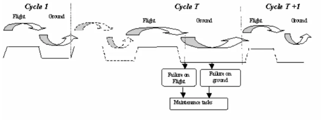
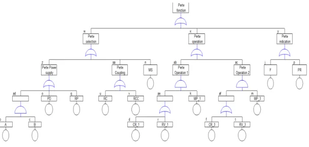
In service, an aircraft is subject to a sequence of cycles with each cycle consisting of a flight phase, followed by a ground phase (which then precedes the next flight). Here we consider an aircraft system made up of a number of various components. During any phase, a component failure may occur. Fig. 1 illustrates the main events that may occur in a sequence of cycles.

(7)

Fig. 1. Operational profile

When a component x fails during cycle T, it may cause the system not to meet the dispatch conditions (safety, operability, commercial...), so-called No Go dispatch

conditions (NG). Formally the occurrence of a NG event is represented by a fault tree, which is based solely on the component states (working or failed). In the case of NG during cycle T, the airline must repair all the components in a state of failure. When a component x fails without involving NG, then two decisions can be made by the airline. Either the airline decides to take off in a so-called Accepted Degraded Mode (ADM), or it refuses the degraded mode (RDM), and then repairs the component that has just failed during cycle T, and does not repair any previously failed component. Note that if a degraded mode is accepted, some minor maintenance tasks configure the component that has just failed. Fig. 2 illustrates all of these different scenarios in detail.

(8)

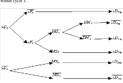
From the two possible states of any given component x at the departure of cycle T: x

works (

xD

_T) or x is failed (

xD

_T ), we display in Fig. 3 all the events that may occur within cycle T.

Fig. 3. The event tree for component x during cycle T.

2.2. Input data

Here is the input data (known quantities) of the in-service aircraft reliability problem: • A coherent fault tree of the system. This fault tree is issued from the system

architecture by design engineers.

•

Pr

{

xF

_T

xD

_T

}

, the probability that component x fails during cycle T, given that

x works at the beginning of cycle T. This quantity is a direct function of the failure rate of component x, which is provided by the component manufacturer.

•

Pr

{

ADM

_T

NG

_T

∩

xF

_T

∩

xD

_T

}

, the probability of accepting the degraded mode, given that x fails during cycle T and that no

NG

_T (i.e.

NG

_T ) occurs. This quantity is a direct function of the pilot behavior and of the airline

(9)

maintenance strategy. It is not a function of the component (see Assumption A7 below).

Note that, due to

NG

_Tevent, ADMT (Accepted Degraded Mode) is not the

complement event of RDMT (Refused Degraded Mode). However, ADMT and

RDMT are conditional complement events, more precisely:

{

ADM

T

NG

T

∩

xF

T

∩

xD

T

}

=

1 −

Pr

{

RDM

T

NG

T

∩

xF

T

∩

xD

T

}

Pr

.

• The initial conditions are also given: we know the state or the probability

{

₁

}

Pr xD

of each component x at the beginning of cycle 1.

2.3. List of assumptions

Here, we list the assumptions induced by both the airline maintenance strategy and the reliability of aircraft systems.

A1. Given the states (working or failed) of each component at the beginning of the cycle T, the component probabilities of failure are independent.

More precisely, the conditional probabilities of failure are independent

while non-conditional probabilities of failure are not. In fact the dependencies

between failure events are due to the NG event occurrence.

A2.The probability of having more than one component failure during each cycle for the system under study is negligible.

Indeed, because our reliability study is dedicated to operational

interruption rate evaluation and due to the fact that we have to deal with highly

reliable components, the above probability is negligible compared with standard

(10)

assumption). This fact is also confirmed by operational interruption rate

estimation throughout airline maintenance data.

A3. A component x is repaired at cycle T only in the following cases:

a. NG occurs during cycle T and component x was in failed state at the departure of cycle T

b. Component x fails during cycle T and NG occurs during cycle T. c. Component x fails during cycle T, NG does not occur during cycle T and the airline refuses the degraded mode for the x component.

A4. When a component is repaired during cycle T, it is assumed to be working at the departure of cycle T+1.

A5. In the cases of NG during cycle T, all the equipments failed before or during cycle T are repaired.

A6. The degraded mode acceptance by the airline during cycle T (ADMT) can occur

when both a component fails and NG does not occur during cycle T. Once a degraded mode has been accepted for component x, it remains failed unless NG occurs during the following cycles.

A7. Given that a component has failed during cycle T without inducing NG, we assume that ADMT (the degraded mode acceptance event) is independent of both

x (the component) and T (the cycle).

Remark that his conditional probability quantity is in practice given by the

airline maintenance strategy and by the pilot behavior. Note that due to the NG

coupling effect, the non-conditional probability of the degraded mode

(11)

A8. The airline refuses degraded mode during cycle T (RDMT) can occur when both

a component fails and NG does not occur during cycle T. Once a degraded mode has been refused for component x, it is repaired and it is assumed to be working at the beginning of cycle T+1.

A9. Given that a component has failed during cycle T without inducing NG, we assume that RDMT (the event that the airline refuses the degraded mode) is

independent of both x and T.

The strictly analogous remark of A7 for ADMT applies also here for RDMT.

A10. The component failure rates are supposed to be different but independent of the cycle (constant through the sequence of cycles).

A11. We assume the following negative dependency property: at the departure of cycle T, the probability that both components x and y are in failed state is smaller than the individual probability product. More formally, let

y

x

S

y

x

,

∈ ,

≠

be two components. Then,

{

xD

T

yD

T

}

Pr

{ } { }

xD

T

Pr

yD

T

Pr

∩

≤

×

.

As a direct consequence, we have the following general result: Let

x ∈

S

and A a subset of the remaining components (

A ⊂

S

with

x ∉

A

). Then,

(

)

{ }

(

)













×

≤





























∩

∈ ∈

I

A y T T A y T T

yD

xD

yD

xD

Pr

.

Remark: this negative dependency assumption is also equivalent to:

For all pairs of components

x

,

y

∈

S

(

x ≠

y

):

{

xD

T

yD

T

}

Pr

{

xD

T

}

Pr

{

yD

T

}

(12)

The negative dependency property is a consequence of both the maintenance

strategy (see Fig. 2), and the fact that we deal with highly reliable components

(see Appendix for a detailed justification).

3. From analytic developments to efficient computation

The objective of this section is to compute at each cycle T estimates of the probabilities of the main events displayed on Fig. 2: NG (No Go dispatch condition on the system), ADM (Accepted Degraded Mode), and RDM (Refused Degraded Mode), which are in-service aircraft reliability indicators at the preliminary design stage. We present our methodology for computing these probabilities in four steps. In Subsection 3.1, we develop recursive analytical formulae (from cycle T to cycle T+1) for the three main-event probabilities

Pr

{

NG

T

}

,

Pr

{

ADM

T

}

, and

Pr

{

RDM

T

}

. However, these formulae rely on two probabilities that are not computationally tractable for real-world aeronautical systems. Thus, in Subsection 3.2 we develop astute bounds on probabilities related to minimal sets of the NG fault tree. These bounds, in turn, allow us in Subsection 3.3 to derive a bounding methodology for the above conditional NG event probabilities. Finally, we put these results together in Subsection 3.4 to derive an overall iterative scheme based on the initial conditions (at cycle T=1) and input data, in order to obtain an algorithm, called BA, for computing tight bounds for the three main-event probabilities. This algorithm does not rely on dynamic fault-tree analysis, and therefore it meets industrial computational time constraints for the systems considered in preliminary design.

(13)

3.1. Probabilities of the main events: recursive formulae

In this subsection, assuming that probability

Pr

{

xD

T

}

is given for all components x in

S, we show how to obtain, from this information, analytic formulae of the main-event probabilities:

Pr

{

NG

_T

}

,

Pr

{

ADM

_T

}

,

Pr

{

RDM

_T

}

, and consequently

Pr

{

xD

_T₊₁

}

for all x in S. The latter probability will enable us to restart the iterative process.

When a NG occurs during cycle T, a component must have failed during this cycle. Therefore, we have:

(

)

U

S x T T T T

NG

xF

xD

NG

∈

∩

=

.

Because the events

{

xF

T

}

_x∈_Sare disjoint (see Assumption A2), we obtain:

{

}

∑

{

}

{

}

{

}

∈

×

∩

=

S x T T T T T T T

NG

xF

xD

xF

xD

NG

Pr

. (1)

Similarly, for the second main event

ADM

_T, we have:

(

)

U

S x T T T T T

ADM

NG

xF

xD

ADM

∈

∩

=

(see Fig. 3). This implies

{

}

∑

{

}

(

{

}

)

{

}

{

}

∈

×

∩

−

×

∩

=

S x T T T T T T T T T T T

ADM

NG

xF

xD

NG

xF

xD

xF

xD

ADM

Pr

1 Pr

Pr

. (2)

Again, from Fig. 3,

U

(

)

S x T T T T T

RDM

NG

xF

xD

RDM

∈

∩

=

and therefore:

{

}

∑

{

}

(

{

}

)

{

}

{

}

∈

×

∩

−

×

∩

=

ADM

NG

xF

xD

NG

xF

xD

xF

xD

RDM

Pr

1 Pr

Pr

. (3)

Finally, in accordance with Fig. 3, we have:

(

T T

) (

T T T T

)

T

xD

NG

ADM

NG

xF

xD

(14)

{

}

{ }

{

( )

}

{

}

(

1 Pr

{

}

)

Pr

{

}

Pr

{

}

.

Pr

₁ T T T T T T T T T T T T T T

xD

xF

xD

xF

NG

xD

xF

NG

ADM

xD

NG

xD

×

∩

−

×

∩

+

∩

−

=

+ (4)

Except for

Pr

{

NG ∩

T

xD

T

}

and

Pr

{

NG

T

xF

T

∩

xD

T

}

, all values involved in the above formulae are known from inputs (see Subsection 2.2) and from the given probabilities

Pr

{

xD

_T

}

_x_∈_S. The next two subsections will address the issue of bounding / approximating these two unknown probabilities.

3.2. Bounds related to minimal set probabilities

The first step for bounding the two unknown probabilities

Pr

{

NG ∩

T

xD

T

}

and

{

NG

T

xF

T

∩

xD

T

}

Pr

, is to exhibit, for each minimal cut set

MC

i and for each minimal path set

MP

j, upper bounds on events

MC

_Ti (all components of

MC

i are failed at the end of cycle T) and on events

MP

Tj( all components of

j

MP

work at the end of cycle T). More precisely, we derive two types of recursive bounds. The first type is related to minimal cuts. In Theorem 1 below, we provide bounds on

{

T T

}

i

T

xF

xD

MC

∩

Pr

and

Pr

{

MC

_Ti

∩

yF

_T

∩

yD

_T

∩

xD

_T

}

for all i,

1 ≤

i ≤

k

, and for all components

x

,

y

∈ ,

S

y

≠

x

. The second type of recursive bounds, given by Theorem 2, relates to minimal paths and provides bounds on

{

T T

}

j

T

xF

xD

MP

∩

Pr

and

Pr

{

MP

_Tj

∩

yF

_T

∩

yD

_T

∩

xD

_T

}

for all j,

1 ≤

j ≤

p

, and for all components

x

y

S

y

(15)

from input data and probabilities

Pr

{

xD

_T

}

,

x

∈

S

. These bounds will be used in Subsection 3.3 in order to estimate the two unknown probabilities

Pr

{

NG ∩

_T

xD

_T

}

and

{

NG

T

xF

T

∩

xD

T

}

Pr

.

Theorem 1.

Consider the ith minimal cut,

1 ≤

i ≤

k

, and two components

x

,

y

∈

S

with

x ≠

y

. We then obtain: i)

{

}

{ }

{

}











∈

≤

∩

∏

≠ ∈

;

,

0 ,

Pr

otherwise

MC

x

if

xD

yD

xD

xF

MC

i T x y MC y T T T i T i ii)

{

}

{

}

{ }











∈

×













×

≤

∩

∏

≠ ≠ ∈

.

,

0 ,

Pr

,

otherwise

MC

y

if

xD

zD

yD

yF

xD

yD

yF

MC

i T y z x z MC z T T T T T T i T i Proof.

Let us consider the event that all components of the minimal cut

MC

i are in failed state during cycle T. If

x ∈

MC

iand x has failed during cycle T, following Assumption A2, we neglect the event that more than one component fail during one phase, and then, we assume that all the other components of this minimal cut have failed before. Thus, we have:

(16)

If we consider the minimal cuts for a cut

MC

ito occur at T, a component i

MC

x ∈

must fail during the current cycle (only one according to Assumption A2), and the other components have to be lost at the beginning of the cycle T. Thus, this event can be rewritten as











∅

∈

∩













=

∩

≠ ∈

.

,

otherwise

MC

x

if

xD

xF

yD

xD

xF

MC

i T T x y MC y T T T i T i

I

Let

x ∈

MC

i,

{

}

.

Pr





















∩













×





















∩













=





















∩













=

∩

≠ ∈ ≠ ∈ ≠ ∈ T x y MC y T T x y MC y T T T T x y MC y T T T i T

xD

yD

xD

yD

xF

xD

xF

yD

xD

xF

MC

i i i

I

The fact that

{

_T _T

}

x y MC y T T T

xD

yD

xF

xD

xF

i

Pr

=

































∩

≠ ∈

I

is due to the probability

independence of failure (A1).

We use the inclusion of events













⊆

∩













≠ ∈ ≠ ∈

I

x y MC y T T x y MC y T i i

yD

xD

yD

and the

overvaluation of their probabilities that can be deduced. Hence, with Assumption A11 (negative dependency) we obtain:

(17)

{

}

{

}

{

}

Pr

{

}

.

Pr

∏

≠ ∈ ≠ ∈

×

≤

































×

≤

∩

x y MC y T T T x y MC y T T T T T i T i i

yD

xD

xF

yD

xD

xF

xD

xF

MC

I

Consequently, with the equality

{

}

{

T T

}

{

T T

}

i T T T i T

xF

xD

MC

xF

xD

xF

xD

MC

∩

=

Pr

∩

×

Pr

∩

Pr

, we conclude.

ii) An analogous development of the previous proof is used to demonstrate the second overvaluation.

Let

y

∉

MC

i

_,

x

∈

S

. The cut cannot occur and we have:

∅

=

∩

_T _T _T i T

yF

yD

xD

MC

. Let

y

∈

MC

i

_,

x

∈

S

. The cut will occur if all the other components are in a failure state at the beginning of the cycle. Thus, we have:

T T T y z x z MC z T T T T i T

yF

yD

xD

zD

yF

yD

xD

MC

i

∩













=

∩

≠ ≠ ∈

I

, Hence, if

y

∈

MC

i

,

x

∈

S

,

(18)

{

}

{

}

Pr

.

Pr

, , ,





















∩

×

≤





















∩

×





















∩

=

∩

≠ ≠ ∈ ≠ ≠ ∈ ≠ ≠ ∈ T y z x z MC z T T T T T y z x z MC z T T T y z x z MC z T T T T T i T

xD

zD

yD

yF

xD

yD

zD

xD

yD

zD

yF

xD

yD

yF

MC

i i i

I

The previous development relies on the fact that

{

T T

}

T T y z x z MC z T T

zD

yD

xD

yF

yD

yF

i

Pr

,

=





















∩

≠ ≠ ∈

I

(from the probability

independence of failures), and on the inclusion of the following events

T y z x z MC z T T y z MC z T T

zD

xD

zD

xD

yD

i i

∩













⊂

∩













∩

≠ ≠ ∈ ≠ ∈

I

, .

Hence, with Assumption A11 (negative dependency) we conclude:

{

}

{

}

{ }

T y z x z MC z T T T T T T i T

yF

yD

xD

yF

yD

zD

xD

MC

i

Pr

,

×













×

≤

∩

_∏

≠ ≠ ∈ .

□

Theorem 2.

Consider the jth minimal path,

1 ≤

j ≤

p

, and two components

x

,

y

∈

S

with

x ≠

y

. Then, we have: i)

{

}

_{

_}









_∈

≤

∩

∏

∈

.

,

Pr

,

0 Pr

_yD

_otherwise

MP

x

if

xD

xF

MP

j MP y T j T T j T

(19)

ii)

Proof.

i) If we consider the minimal paths, we exploit the observation that one component must fail during the current cycle in order to prevent all minimal paths from occurring. Again, using Assumption A2, the other components necessarily work at the beginning of the cycle. Thus, for any component

x ∈

S

, we have:











∩













∈

∅

=

∩

∈

.

,

otherwise

xD

xF

yD

MP

x

if

xD

xF

MP

T T MP y T j T T j T j

I

The next development relies on (the remark in) Assumption A11, and on the fact that

{

T T

}

MP y T T T

xD

yD

xF

xD

xF

j

Pr

=





























∩

∈

I

(from the probability independence

of failures, Assumption A1):

{

}

{

}

{

}

{

}











×

















×

∈

≤

∩

∏

∈

.

,

Pr

,

0 Pr

otherwise

xD

yD

xD

xF

MP

x

if

xD

xF

MP

T MP y T T T j T T j T j

ii) We use a development analogous to that of the previous proof to demonstrate the second overvaluation.

{

}

{

}

{

}

{

}

{

}

{ }























×













×

∈

≤

∩

∏

∈

.

,

Pr

,

Pr

min

,

0 Pr

otherwise

xD

yD

yF

yD

zD

yD

yF

MP

y

or

MP

x

if

xD

yD

yF

MP

T T T T MP z T T T j j T T T j T j

(20)

The event is divided as follows:











∩













∈

∅

=

∩

∈

,

otherwise

xD

yD

yF

zD

MP

y

or

MP

x

if

xD

yD

yF

MP

T T T MP z T j j T T T j T j

I

but we cannot apply Assumption A11 to conclude directly.

On the other hand, with

x

,

y

∉

MP

j, we have the following two inclusions:

,

T T MP z T T T T j T

yF

yD

xD

zD

yF

yD

MP

j

∩













⊆

∩

∈

I

.

T T T T T T j T

yF

yD

xD

yF

yD

xD

MP

∩

⊆

∩

From the first inclusion, with (the remark in) Assumption A11, we obtain the following overvaluation:

{

}

{

}

{

}

{

_T

}

MP z T T T T T T j T

yF

yD

xD

yF

yD

zD

yD

MP

j

Pr

_

×











×

≤

∩

_∏

∈ .

From the second one, we use the inclusion

yD

_T

∩

xD

_T

⊂

xD

_T to obtain the following overvaluation:

{

j _T _T _T

}

{

_T _T _T

}

{

_T _T

}

{

_T _T

}

{ }

_T

T

yF

yD

xD

yF

yD

xD

yD

xD

yF

yD

xD

MP

Pr

∩

≤

∩

×

∩

≤

×

We take the minimum of both overvaluations to conclude.

□

Remark: For highly reliable systems, the second overvaluation is more efficient than the

first one. It corresponds to the following inequality:

{

}

{

}

{ }

_T MP z T T

zD

xD

yD

j

Pr

×

∏

≥

∈ .

(21)

3.3. Bounds related to No Go dispatch condition probabilities

Here, we show how to bound the unknown probabilities

Pr

{

NG ∩

T

xD

T

}

and

{

NG

T

xF

T

∩

xD

T

}

Pr

of Subsection 3.1. More precisely, upper bounds will be derived

in Theorem 3, using a minimal cut-set decomposition and Theorem 1 (Subsection 3.2). Then, using a minimal path-set decomposition and using Theorem 2 (Subsection 3.2), we

shall derive lower bounds in Theorem 4. Note that all the bounds on

Pr

{

NG ∩

T

xD

T

}

and

Pr

{

NG

_T

xF

_T

∩

xD

_T

}

given by Theorems 3 and 4 can be computed from input data and the probabilities

Pr

{

xD

T

}

,

x

∈

S

.

Theorem 3.

For any component

x ∈

S

, we have:

i)

{

}

{ }

{

}

{

}

∑

∏

= ∈ ≠ ∈

×

≤

∩

k i MC x T x y MC y T T T T i i

xD

yD

xD

xF

NG

1

1 Pr

Pr

, (5) where

_{

_}







_∈

=

∈

.

0 ,

1 :

1 otherwise

MC

x

if

i MC x i ii)

{

}

{ }

{

}

{ }

{

}

{

}

























×

≤

∩

∑

∏

≠ ∈ = ∈ ≠ ≠ ∈ x y S y k i MC y T y z x z MC z T T T T T T i i

yD

zD

yD

yF

xD

NG

1

1 Pr

Pr

. (6)

(22)

Proof.

i) Let us consider the failure of a component x. In order to have a NG, at least one minimal cut which contains x must occur. Thus, using the general addition theorem

bound and the fact that

U

k i i T T

MC

NG

1 =

=

, we have, for any component

x ∈

S

:

{

}

{

}

{

}

1 _{

_}

.

Pr

1 1 1

∑

= ∈ = =

×

∩

≤

∩

≤













∩

=

∩

k i MC x T T i T k i T T i T T T k i i T T T T i

xD

xF

MC

xD

xF

MC

xD

xF

MC

xD

xF

NG

U

Hence, from Theorem 1, we obtain an upper bound for the NG probability given failure of a component

x ∈

S

during cycle T:

{

}

{ }

{

}

1 {

}

.

Pr

1

∑

∏

= ∈ ≠ ∈

×

≤

∩

xD

yD

xD

xF

NG

Of course, we can also obtain an upper bound for the NG probability using the previous overvaluation and Eq. (1).

ii) Based on formulation (1) of NGT event, an analogous development can be applied to

the event

NG ∩

_T

xD

_T to obtain the following overvaluation:

(

)

U

x y S y T T T T T T

xD

yF

yD

NG

xD

NG

≠ ∈

∩

=

∩

.

(23)

{

}

{

}

(

)

{

}

{

}

{ }

{

}

{

}

∑

∏

∑∑

∑

≠ ∈ ∈ ≠ ∈ ≠ ∈ = ≠ ∈ = ≠ ∈

×













×

≤

∩

≤

















∩

=

∩

=

∩

x y S y MC y T y x z MC z T T T T x y S y k i T T T i T x y S y k i T T T i T x y S y T T T T T T i i

yD

zD

xD

yD

yF

xD

yD

yF

MC

xD

yD

yF

MC

xD

NG

yD

yF

xD

NG

,

1 Pr

Pr

, 1 1

U

with the remarks:

•

Pr

{

yF

_T

yD

_T

∩

NG

_T

∩

xD

_T

}

=

Pr

{

yF

_T

yD

_T

}

•

yD

_T

∩

xD

_T

⊂

xD

_T , which implies the overvaluation.

□

Theorem 4.

For any component

x ∈

S

, we have:

i)

{

}

∑ ∏

{

}

_{

_}

= _∈ ∉

×













−

≥

∩

p j _y _MP x MP T T T T j j

yD

xD

xF

NG

1

1 Pr

(7)

(24)

ii)

{

}

{

}

{

}

{ }

{

}

{

}

{

}

{

}

{ }

{

}

{

}

.

1

1 Pr

Pr

,

Pr

min

Pr

, 1

∑ ∑

∏

∑

≠ ∈ ∉ = ∈ ∈ ∈ ≠ ∈













×













×













×

−

×

≥

∩

x y S y p MP y x j MP x MP y T T T T MP z T T T x y S y T T T T T T i j j j

xD

yD

yF

yD

zD

yD

yF

xD

yD

yF

xD

NG

(8) Proof.

Let us consider the failure of a component x. In order to have a NG, all the minimal paths not containing x, do not occur at the beginning of the cycle.

i) If we consider the failure of a component x, to have a NG, Thus, using the general

addition theorem bound and the fact that

I

p j j T T

MP

NG

1 =

=

, we have for any

component

x ∈

S

:

{

}

{

}

.

Pr

1 Pr

Pr

1 1 1

∑

= = =

∩

−

≥

















∩

−

=

















∩

=

∩

p j T T j T T T p j j T T T p j j T T T T

xD

xF

MP

xD

xF

MP

xD

xF

MP

xD

xF

NG

U

I

Hence, from Theorem 2, we obtain an upper bound for the NG probability given failure of a component

x ∈

S

during cycle T:

(25)

{

}

1 Pr

{

}

1 _{

_}

.

Pr

1

∑ ∏

= _∈ ∉

×













−

≥

∩

p j _y _MP x MP T T T T j j

yD

xD

xF

NG

ii) Based on formulation of NG event from Eq. (1) of the NG event, an analogous

argument can be applied to the event

NG ∩

_T

xD

_T to obtain the following development: T T T p MP y x j j T T T T T

yF

yD

xD

MP

yF

yD

xD

NG

j T

∩













=

∩

∉ =

I

, 1 .

From the fact that

Pr

{

yF

T

yD

T

∩

xD

T

}

=

Pr

{

yF

T

yD

T

}

(from the probability of independent failures), and using Theorem 2, we derive the following development:

{

}

{

}

{

}

{

}

{

}

{

}

{ }

{

}

∑

≠ ∈ ∉ = ≠ ∈ ∉ = ≠ ∈ ∉ = ≠ ∈ ≠ ∈













∩

−

×

≥





































∩













−

∩

=





















∩

=

∩

=

∩

=

∩

x y S y p MP y x j T T T j T T T T T x y S y T T T p MP y x j j T T T T x y S y T T T p MP y x j j T x y S y T T T T x y S y T T T T T T j j j

xD

yD

yF

MP

xD

yD

yF

xD

yD

yF

MP

xD

yD

yF

xD

yD

yF

MP

xD

yD

yF

NG

xD

yD

yF

NG

xD

NG

, 1 , 1 , 1

Pr

U

I

□

(26)

3.4. The Bound Algorithm (BA) for computing operational interruption rate indicators

In this Subsection, we present recursive formulae for evaluating (lower and upper) bounds on probabilities of the three main events:

NG

_T (a No Go dispatch condition occurs during cycle T),

ADM

_T (the airline Accepts the Degraded Mode for take-off at the beginning of cycle T+1), and

RDM

T (the airline Refuses the Degraded Mode for take-off at the beginning of cycle T+1) at each cycle T. These formulae derive from the recursive equation (4) of Subsection 3.1 and from the bounds provided by Theorems 3 and 4. These main event probability bounds can easily be computed from the given input data (including the given initial conditions at cycle 1,

Pr xD

{

₁

}

, for all component x in

S.---see Subsection 2.2). From a straightforward application of Bayes rule, we obtain the following formulae:

(

)

∑

(

)

{

}

(

)

∈

×

∩

=

S x T T T T T T T

UB

NG

xF

xD

xF

xD

UB

xD

NG

UB

Pr

(

)

∑

(

)

{

}

(

)

∈

×

∩

=

S x T T T T T T T

LB

NG

xF

xD

xF

xD

LB

xD

NG

LB

Pr

(

)

∑

{

}

(

)

{

}

(

)

∈

×

∩

−

×

∩

=

ADM

NG

xF

xD

LB

NG

xF

xD

xF

xD

UB

xD

ADM

UB

Pr

1 Pr

(

)

∑

{

}

(

)

{

}

(

)

∈

×

∩

−

×

∩

=

ADM

NG

xF

xD

UB

NG

xF

xD

xF

xD

LB

xD

ADM

LB

Pr

1 Pr

(

)

∑

(

{

}

)

(

)

{

}

(

)

∈

×

∩

−

×

∩

−

=

ADM

NG

xF

xD

LB

NG

xF

xD

xF

xD

UB

xD

RDM

UB

1 Pr

(

)

∑

(

{

}

)

(

)

{

}

(

)

∈

×

∩

−

×

∩

−

=

ADM

NG

xF

xD

UB

NG

xF

xD

xF

xD

LB

xD

RDM

LB

1 Pr

where:

(27)

(

)

( )

(

)

{

}

∑

∏

= ∈ ≠ ∈

×

=

∩

xD

LB

yD

UB

xD

xF

NG

UB

1

is obtained from inequality (5), and

(

)

∑ ∏

(

)

_{

_}

= ∉ ∈

×

−

=

∩

p j MP x MP y T T T T j j

yD

UB

xD

xF

NG

LB

1

is obtained from inequality (7).

The above bounds on the three main-event probabilities can be computed from input data, because