HAL Id: hal-01803000
https://hal-enpc.archives-ouvertes.fr/hal-01803000
Submitted on 24 Apr 2019HAL is a multi-disciplinary open access archive for the deposit and dissemination of sci-entific research documents, whether they are pub-lished or not. The documents may come from teaching and research institutions in France or abroad, or from public or private research centers.
L’archive ouverte pluridisciplinaire HAL, est destinée au dépôt et à la diffusion de documents scientifiques de niveau recherche, publiés ou non, émanant des établissements d’enseignement et de recherche français ou étrangers, des laboratoires publics ou privés.
Magnetic resonance imaging evidences of the impact of
water sorption on hardwood capillary imbibition
dynamics
Meng Zhou, Sabine Caré, Denis Courtier-Murias, Pamela Faure, Stéphane
Rodts, Philippe Coussot
To cite this version:
Meng Zhou, Sabine Caré, Denis Courtier-Murias, Pamela Faure, Stéphane Rodts, et al.. Magnetic res-onance imaging evidences of the impact of water sorption on hardwood capillary imbibition dynamics. Wood Science and Technology, Springer Verlag, 2018, 52 (4), pp.929-955. �10.1007/s00226-018-1017-y�. �hal-01803000�
1 Magnetic resonance imaging evidences of the impact of water sorption on hardwood
capillary imbibition dynamics
M. Zhou, S. Caré, D. Courtier-Murias, P. Faure, S. Rodts, P. Coussot
Université Paris-Est, Laboratoire Navier (ENPC, IFSTTAR, CNRS), Champs sur Marne, France
Abstract: Imbibition in poplar wood is studied from macroscopic measurements (mass and deformation) along with Magnetic Resonance Imaging (MRI) experiments allowing to observe bound and free water dynamics. Additional experiments with silicone oil allow to compare the characteristics of water imbibition with those of a liquid not hygroscopically adsorbed in wood. It was shown that, in contrast to porous media with an impermeable solid structure, the water imbibition in the hydraulic conduits of hardwood is not simply driven by the standard capillary effects associated with a good wetting of the solid surface, but it is in fact strongly affected by the adsorption of bound water in cell walls. More precisely bound water appears to progress far beyond the front of free water, and the free water penetration along the sample axis apparently coincides with the development of a region saturated with bound water. This likely explains that water imbibition is about three orders of magnitude slower than expected from standard Washburn imbibition process.
Introduction
Liquid transport in wood plays a major role with regard to its properties in various situations. It contributes to the functioning of tree, through the sap ascent towards the leaves. Liquid impregnation of wood pieces is used for treatment (Mader et al. 2011; Carrillo et al. 2012; Bessières et al. 2013) often in combination with high temperature or pressure, or consolidation (Kucerova 2012). Wood products or structures are subjected to variable environmental conditions leading to water migration which might have an impact on their mechanical properties. As the structural integrity may be compromised for wood products or structures if the induced properties such as swelling or shrinkage are badly evaluated (Kretschmann 2003; Van Houts et al. 2004; Silva et al. 2014), and for trees if cavitation occurs (Vincent et al. 2012, 2014; Ball 2014), the liquid migration process has to be better understood. The mechanisms of liquid transport are related to the hierarchical and multiscale structure of wood. Wood is composed of tubular cells, with different void (or lumen) sizes and arrangements (tracheids for softwood, vessels and fibers for hardwood), connected by pits, and with characteristics depending on the localization within the growth ring (latewood or earlywood) in the case of wood from temperate regions.
Liquid transport in a porous medium is basically described by the Darcy’s law, which tells us that the pressure gradient is equal to the flow rate times the fluid viscosity divided by the medium permeability. The permeability basically scales with the square of the pore size, but for materials such as wood exhibiting a multi-scale structure the permeability can reflect the different classes of void sizes (Siau 1984) and/or the alternating of voids and (bordered or simple) pits (Petty 1981; Choat et al. 2008). Imbibition dynamics in a porous medium is also governed by a pressure gradient due to the capillary pressure (determined by the air-liquid menisci at the imbibition) and acting over an increasing distance. However, some curious effects have been reported with wood in the sense that they are not expected with homogeneous porous media made of a solid impermeable structure: an apparent behavior similar to that resulting from the existence of two (Petty 1975) or three (González and Siau 1978) media of different void sizes being impregnated in parallel; a permeability decrease with the sample length increase (Bramhall 1971; Bolton 1988; Krabbenhoft 2003; Choo et al. 2013), the penetration of a non-straight front (Krabbenhoft 2003; Salin 2008b) in contradiction with the expected standard Washburn capillary imbibition (Washburn 1921; Gruener et al. 2012), and an apparent permeability (via imbibition tests) much smaller than predicted from a simple analysis of the structure (Perré 2000). Finally, there
2 does not seem to exist a comparison of data with the prediction of imbibition properties based on Washburn model and a well-identified intrinsic permeability deduced from the observations of liquid (sap) transport properties under saturated conditions.
Recently results from MRI (Almeida et al. 2008), vapor adsorption (Dvinskikh et al. 2011) or imbibition (Kekkonen et al. 2014; Mazela et al. 2014), and from neutron radiography for imbibition (Sedighi-Gilani et al. 2012, 2014; Desmarais et al. 2016), showed that in softwoods the water preferentially advances through the latewood. However, the origin of the water dynamics was not studied but some effects suggested some interplay between free and bound water transfers. One of the greatest advantage of MRI is its ability to distinguish different states of water in wood with the help of relaxometry (Menon et al. 1987; Labbe et al. 2002; Gezici-Koç et al. 2017). With such tools a recent work (Gezici-Koç et al. 2017) investigated the free and bound water transport during both water uptake and drying, and confirmed that bound water diffusion within cell walls plays an important role in water transfers in wood. This finally led Gezici-Koç et al (2017) to describe the water transport in terms of a phenomenological process which relies on a diffusivity globally resulting from vapor, free and bound water transport, leaving apart fundamental knowledge of capillary dynamics in porous media.
In the present work, the impact of different parameters (initial water content in wood, the viscosity, surface tension and polarity of liquids) on the flow dynamics is studied and the consistency of these results with regards to usual analysis in the frame of liquid transport in porous media is discussed. In order to explain the problems observed we then take an in-depth look at the imbibition characteristics in the material with MRI, in particular, distinguishing bound and free water dynamics and correlating them to the macroscopic deformations, and measuring their respective distribution profiles (along the sample axis) in time. Besides water, a non-polar silicon oil not hygroscopically adsorbed in wood is also studied in order to eliminate the interactions between the imbibed liquid and the wood cell walls. It was shown that the mechanism of water imbibition in wood is not at all a penetration basically due to capillary effects associated with the size of the main voids, it is rather fundamentally driven by bound water adsorption in cell walls.
Materials and Methods Wood Samples
Heartwood specimens were collected from poplar wood (Populus Canescens, cut in 2014, from northeastern region of France). Poplar is a diffuse-porous hardwood which means that its vessels are homogenously distributed within growth rings. For standard imbibition tests and MRI experiments, samples were sawn along the anisotropic directions of wood to give 10 cm in longitudinal (L) direction, which is parallel to the imbibition axis, and 4 × 1.6 cm2 in radial (R) and tangential (T) direction
respectively, with 7-8 visible growth rings. The density of dry poplar samples at room temperature is 0.469 ± 0.013 g/cm3. For droplet imbibition tests and sample characterizations, small cubic samples
about 1 cm3 were also prepared. All the samples were taken side by side in order to minimize the
3 Figure 1 : (A, B, C) Scanning electron microscope images of the TL plane in secondary electron imaging mode. (D) Dark-field microscopy image of the transversal cross-section: fibers and some vessels were possibly filled with wood powder during the polishing. Vessels (stars in A, B and D) are visibly much larger than fibers (circles in A, C and D) and with no tylose inside. Vessels with simple perforation plates (circular openings indicated by squares in B) may be considered a priori as continuous (B). Fibers (e.g. white disk in C) are discontinuous with a few pits on the walls (small black points indicated by the arrows). Wood rays are also visible in the image D (horizontal rays) but their volume and role during longitudinal imbibition are negligible.
Each sample is initially stored until equilibrium thanks to a saturated Mg(NO3)2 solution which
ultimately gives a RH (Relative Humidity) of 53% at room temperature (25°C). Thus, the wood samples reach a constant moisture content (MC) (water to dry wood mass ratio) of 9 ± 0.06%. A saturated K2SO4
solution is also prepared and provides a RH of 97% at 25°C.
Sample porosity and morphology, fiber and vessel diameter are characterized by optical and scanning electron microscopies. The transversal cross-section of samples is carefully polished with sandpapers whose grit size varies from P200 down to P4000 (number of grains per cm2) for the optical observations
and the samples were cut with wood chisels to obtain fractured surfaces and carbon-coated for the SEM observations. Image analysis is carried out using ImageJ software (Schneider et al. 2012), over a wide series of images taken from different annual rings. The distribution of lumen radius shows essentially two peaks centered around 55 µm and 8 µm, which correspond to the average diameter of vessels and fibers, respectively. These data show that the poplar samples consist of 40 ± 5% of vessels, 29 ± 4% of fibers and 31 ± 2% of cell walls (see Appendix A in Electronic Supplementary Material), giving a total porosity of 70%. This value of porosity with the normal 1500 kg/m3 for cell wall density lead to a sample
4 In hardwood species only vessels are considered to have sap conduction function. For poplar, tyloses that could block the flow are rarely presented, and its vessel elements are connected to each other by simple perforation plates (Wheeler et al. 2007). By this means the vessels in poplar are practically considered as long capillary tubes in parallel (a priori longer than the sample size, i.e. 10 cm) (see Figure 1). In addition poplar contains fiber parallel to vessels and of typical length between 900-1600 µm (data collected from InsideWood database; Wheeler 2011) (see Figure 1). There appear to be a few pits dispersed along the fibers (see Figure 1.C). The existence of some pits along the vessels cannot be excluded, but they were not observed in the RL and TL planes. Finally, there is a porous structure made of long and large channels through which the liquid can a priori rapidly progress, and a second porous network situated around these channels where the liquid may penetrate more slowly, either via pits or by diffusion through cell walls. The small size and numbers of the vessel-to-fiber pits substantially reduce the effectiveness of free liquid flow (Bonner and Thomas 1972). In this study, the secondary penetration will be a subject of discussion. Anyway, one is dealing with a porous medium, i.e. a solid structure with voids, for which it is natural to expect a Washburn imbibition process (Washburn 1921; Gruener et al. 2012), namely a penetration driven by capillary (Laplace) pressure due to menisci formed by the air-liquid interface inside the porous medium, and a viscous resistance due to liquid flow through the lumens.
Standard imbibition tests
The standard imbibition test consists of suspension of a wood sample from a scale and immersion of its bottom (over about 3-5 mm) in a deionized water bath inside a container, whose cross-section is much larger than that of the wood sample (see Figure 2). A cover (not in contact with the sample) was placed over the free surface of water to limit the evaporation which was then, from independent tests, shown to be negligible. To avoid capillary effects between the external wood surface and the water bath, each sample was sealed with a commercial liquid-impermeable painting (Aqua-Stop®) along the four vertical sides parallel to the imbibition direction (see Appendix B in ESM). A 1 g/L aqueous solution of betaine was prepared with a smaller surface tension (0.03 N/m) to examine the impact of the surface tension for water. Imbibition tests with four silicon oils obtained from Chimie Plus were also carried out. Their specific gravity to water, viscosity and surface tension at 25°C were: -1
N.m 0.0206 Pa.s, 0.02 , 95 . 0
(47V20), 1.065 ,0.125Pa.s,0.0245N.m-1(125), 0.97 ,0.35Pa.s,0.0211N.m-1(47V350), and -1 N.m 0.021 Pa.s, 0.5 , 97 .
0 (no commercial name). The experiments were carried out at room temperature (25°C).
The apparent mass of water entering the sample from the initial state was measured by the scale in time with intervals not less than 1 s. Due to a buoyancy force varying with the water level in the bath, the apparent mass should be corrected to get the effective mass absorbed by the sample, which writes (see Appendix C in ESM)
(
S Sb)
m
m= 0 1− (1)
where
m
0 is the apparent mass, m the effective mass of uptaken liquid,S
the cross-section area of the wood sample andS
bis the cross-section area of the liquid bath.5 Figure 2 : Scheme of the imbibition test.
“Washburn analysis” of imbibition tests
The standard imbibition test is generally expected to provide information on the characteristics of the porous media. In the simplest case, the liquid penetration corresponds to a “Washburn imbibition” (Washburn 1921). In this context, the liquid is driven by a capillary force due to the menisci along the air-liquid interface at the front of penetration inside the sample, and the sample is filled with liquid behind this front. As a consequence, the capillary driving force is constant, but it must act over an increasing distance of penetration, so that the flow rate progressively decreases. More precisely, it can be considered that at the front (interface) the average capillary pressure (neglecting ambient pressure), scales as:
R p=σcosθ α
∆ (2)
where σ is the surface tension,
θ
the contact angle, R a characteristic pore radius and α a factor related to the pore shape. This driving force acts over a distance of penetration h, which induces apressure gradient p h. Darcy’s law then expresses the balance between the pressure gradient and the
viscous resistance: V k h p µ = ∆ (3)
where µ is the liquid viscosity (10−3Pa.s for water),
V the mean flow velocity through the sample, and
k the permeability of the porous medium. Assuming that the liquid advances as a front saturating the voids below a distance h=Ω εS increasing in time (where Ω is the volume of water entered in the
sample), V =
(
dΩ dt)
S =ε(
dh dt)
, withε
the (accessible) medium porosity. The solution of the resulting differential equation (3) for the apparent distance of penetration of the liquid front isµ λ t S= Ω (4) with R kεσ θ α λ= 2 cos (5)
The above approach neglected gravity effects. When taking them into account the driving force is damped by a term
ρ
gx so that Darcy’s law now writes:6 V k g h p ρ µ = − ∆ (6)
The solution of this equation now expresses as: ) 1 ln( h B B h AB t − − − = (7)
with A=µε kρg and B=σcosθ αRρg. The solution without gravity is recovered from (7) when h
is much smaller than B , but finally
g R h h ρ α θ σcos max = → when t→∞ (8)
Note that in the tests the sample is partially immersed to a depth (∆hw), which induces an additional
pressure term, ρg∆hw, in ∆p. This term is in general negligible in the first (capillary) regime, but it may
play a role in the second regime, then ∆hw must be withdrawn from the above maximum height expression.
For the flow through a cylindrical capillary,
α
=1/2 (the meniscus is a spherical cap) and the velocity profile can be computed exactly (Poiseuille law), which directly gives the relation between the pressure gradient and the mean velocity, from which the permeability is deduced for a set of parallel capillaries:8
2
R
k=
ε
.Droplet imbibition
Another imbibition test was also used which consists of measuring the evolution of the geometry of a droplet deposited on the transversal cross-section of a wood sample. In this case, prior to the test, the sample cross-section was carefully polished with a sandpaper P400 to reduce the surface roughness. The evolution of the droplet shape after deposition was recorded by a 30 fps camera. It appeared that the droplet almost instantaneously spreads and reaches a fixed area of contact with the wood surface, i.e. the line of contact did not move significantly during imbibition. The droplet shape is well represented by a spherical cap, so that by tracing the height and diameter of the cap as a function of time, the variation of the volume of liquid (Ω) per unit (initial) cross-section area (S) in contact with liquid, was obtained as a function of time ( t ). This test is specifically appropriate for wood. Indeed, due to the wood structure the liquid penetrates essentially along the longitudinal direction so that the theoretical description for 1D capillary imbibition should still apply.
Deformation measurements.
For imbibition tests, sample deformations are measured with an outside micrometer Mitsutoyo with 0.01 mm precision in the transversal plane (radial and tangential directions) every 5 mm along the sample axis. Note that it is reasonable to consider that the measurements are performed at the same position along the sample axis (fiber direction) since the longitudinal deformation is less than 1% between RH 53% and 97% (parallel measurements made on samples).
NMR relaxometry.
To identify different water states in wood, NMR relaxation measurements were performed at 20°C with a BRUKER MINISPEC MQ20 spectrometer operating at 0.5 T (20 MHz for 1H). The NMR
spectrometer enables the analysis of samples with a maximum diameter of 18 mm and a maximum height of 10 mm. Samples were cut into about 1 cm3 and put into an 18-mm glass tube which was then
7 days before) were performed using a Carr-Purcell-Meiboom-Gill (CPMG) NMR experiment by carrying out 5000 echoes with an echo time of 0.5 ms. Then, NMR data was post-treated by means of an inverse Laplace transform (ILT) algorithm, which converts relaxation signal into a continuous distribution of relaxations, providing T2 distribution spectra. This was done by using a homemade computer program
based on the method described by Whittall and MacKay (1989) and performing the same work as the CONTIN program by Provencher 1982. Further details about the technique can be found in the work by Faure and Rodts (2008). As can be seen in Figure 3, three well separated T2 relaxation distributions were
observed with maximum values of 4, 60 and 550 ms. The fast-relaxed signal (4 ms) is attributed to bound water and the two peaks at 60 and 550 ms are considered as free water. (Menon et al. 1987, 1989; Labbe et al. 2002). 10-1 100 101 102 103 104 0 2 4 6 8 10 R M N i n te n s it y ( a .u .) T2 (ms)
Figure 3 : T2 distribution of wood sample immersed in water after 3 days.
The decrease of the T2 value for bound water with the moisture content in wood samples has been
reported by many authors, both for hardwood (Almeida et al. 2007; Passarini et al. 2014) and softwood (Menon et al. 1987; Cox et al. 2010; Bonnet et al. 2017). In order to investigate this tendency with the poplar samples, CPMG experiments were further conducted with wood samples hygroscopically equilibrated at 53% RH and 97% RH, respectively. CPMG echo train comprised successive echoes with an echo time of 0.06 ms, among which 200 echoes were recorded following an approximately geometric series from 0.06 ms to 12 ms. Figure 4 shows the measured T2 distribution. Two main peaks could be
identified: the fast peak with a T2value lower than 0.1 ms corresponds to wood polymers (Bonnet et al.
2017), and the slowest peak (1 ms for sample equilibrated at 53% RH and 4 ms for 97% RH) corresponds to bound water absorbed within cell walls. Note that the fast-relaxed polymer peak is not quantitative because of the first measurement taking place at 0.06 ms, however, the displacement of the bound water peak with the relative humidity can be clearly observed. This may be explained by an increased mobility of water molecules in cell walls, with higher water content (Bonnet et al. 2017).
8 10-2 10-1 100 101 0 50 100 150 200 250 300 bound water R M N I n te n s it y ( a .u .) T2 (ms) polymer
Figure 4 : T2 distribution of wood samples equilibrated at 53% RH (squares) and 97% RH
(circles).
Magnetic Resonance Imaging. Set up
A wood sample was immersed in liquid (water or oil) about 1 cm depth in an 800 ml glass beaker and the surface of the container was covered by parafilm to avoid evaporation during 3-day measurements. The beaker together with the sample was put on a plastic sample support whose vertical position can be adjusted in order to be placed inside the MRI system. The distribution of liquid content along the sample axis (see Figure 5) was measured by a vertical MRI spectrometer (DBX 24/80 Bruker) operating at 0.5 T and equipped with a 1H birdcage radio frequency coil of 20 cm inner diameter. As NMR relaxation
times depend on magnetic field strength, they are in principle the same in both NMR relaxation and MRI experiments since both the equipments have the same magnetic field. The magnetic gradient is applied along the vertical axis.
Figure 5 : (a) Projection of transverse signal for 1D profiles along sample axis and (b) slice selection for 2D NMR imaging. For 1D profiles, every point corresponds to the integrated signal in the horizontal slice (shown as the light gray cuboid) with 1.25 mm of thickness.
9 2D imaging is realized as a vertical slice with 2 mm of thickness (in the tangential direction) parallel to the RL plane.
1D Imaging sequence
The NMR profiling sequence utilized in this study measured 8 echoes making use of a 32 steps duplex cogwheel phase cycling scheme (Levitt et al. 2002) acting on π pulses only to select desired coherence pathways. The experiment was performed at the magnetic center of the gradient coil (a BGA26 Bruker, 26 cm inner diameter) with a field of view of 20 cm. The resolution along the vertical axis is 1.25 mm. Slight profile distortion due to possible gradient non-linearity was observed. To eliminate this distortion, all the profiles were normalized by a referential profile of a cylinder glass tube with known dimensions containing the same liquid. The measurements were not subjected to any spin-lattice NMR relaxation (T1) weighting, because the recycling delay between scans was set to 5 times of the longest T1 of water
found in the present sample. The gradient strength was about 0.035T.m-1 with 500 μs stabilizing time
and freshly tuned pre-emphasis which removes eddy effects at the end of this stabilizing time. Echo time (which also more or less corresponds to the time length of each echo recording) was equal to 3.47 ms. Since the T2 value of bound water at low RH % was relatively fast (see Figure 4), the quantification of
bound water content was not exact or even null at low RH %. However, at high RH %, the T2 of bound
water increased to a value of about 4 ms (see Figure 4). Thus, the bound water content was well quantified thanks to the extrapolation of the echoes measured with the present experiment (see below for further details on data treatment). This means that bound water can be expected to be quantitatively well measured in the NMR profiles in the case of higher concentration of bound water. On the contrary, in the regions of lower bound water content, the NMR signal is no longer proportional to the bound water content, but it is seen that it is still possible to study quantitatively the bound water dynamics from the shape evolution of the NMR signal distribution along the sample height. Due to the significant contrast between the signal from bulk liquid and the signal inside the sample, the profiles oscillate around the real value at the borders (liquid interfaces) of bulk liquid. MRI signal was multiplied by a Gaussian function to reduce these oscillation effects.
For silicon oil, the surface relaxivity (the proportionality constant between T2 decay time and pore size)
is very small so that the influence of the pore size on the T2 relaxation time of silicon oil within the
present measurement could be neglected. The T2 value of the bulk liquid is at 517 ms while in the pores
it only shows one peak around 504 ms. As a consequence, for silicon oil measurements only the first echo of silicon oil was used for the data exploration.
To remove the spurious contribution of T2 relaxation and to separate signal between bound and free
water, it was proceeded in a similar manner to that previously done by Menon et al. (1989). With the help of the T2 distribution in Figure 3, a bi-exponential relaxation (permitting a more robust fit than a
tri-exponential fit with the present data) in each layer of the sample could be assumed to separate bound and free water. Thus, MRI data can be represented as if in each layer of the sample it was affected by local relaxation T2,b(z) and T2,f(z) (corresponding to relaxation of bound and free water). In addition,
with m0,b(z) and m0,f(z) referring to the actual spin density profile of bound and free water respectively,
the profiles obtained from each n echo were modeled as:
( )
( )
( )
( )
( )
− + − = z T nTE z m z T nTE z m z prof f f b b n , 2 , 0 , 2 , 0 exp exp (9)with TE the echo time.
To estimate the error of this approach synthetic MRI data were generated representing relaxation information found in Figure 3 having a similar noise level as that of the current MRI measurements. Then, this artificially generated NMR signal was fitted by a bi-exponential function and the obtained amplitudes were compared to the experimental amplitudes from Figure 3. The resulting uncertainty is less than 3%.
10 Note that a tri-exponential fit could also be considered to get even more information on the internal processes. Unfortunately, the relevance of such an analysis is quite limited by the limited number (i.e. 16) of echo, the signal to noise ratio, and the evolution of the T2 values for the two peaks of free water.
These different effects do not allow to get a clear distinction of the evolution of these two species. Anyway it does not seem really useful to distinguish the possible two types of free water, as one is unable to understand the origin of these two populations of water. It would be natural to consider that they correspond to the two types of structural elements according to pore sizes: the medium peak would correspond to free water in fibers while the other one to free water in vessels. However, the ratio of the intensity of the two peaks does not correspond to the volume ratio of fibers and vessels as measured by image analysis of microscopic observations, so that it cannot be definitely concluded on that point. As a consequence, it is preferable to speak of free water as a whole and avoid trying to distinguish two populations without clear physical interpretations.
2D imaging
Five simultaneous 2D MRI vertical slices of 2 mm thickness with 2 mm interval between them (parallel to RL plane, see Figure 5) passing through the wood sample with space resolution equal to 0.47 (radial) × 2.19 (longitudinal) mm, were taken at different times during wood imbibition. A spin multi-echo (MSME) pulse sequence acquiring 8 multi-echoes was used with an multi-echo time of 10 ms and a recycle delay of 600 ms. A short recycle delay value and multi-echo addition were chosen so as to obtain an acceptable signal-to-noise ratio and to keep measurement time below 30 minutes. It however induces both T1- and T2-weighting, thus preventing here direct quantification. Moreover, they do not show bound
water as its T2 value is of the order of 4 ms. 2D images are thus essential to appreciate the distribution
of liquid in the transversal direction but can only be qualitatively compared with 1D profiles of free water.
Results and discussions Oil imbibition
Let us first look at the results obtained from the imbibition tests with silicone oil. No swelling of the sample was observed. This confirms that oil does not penetrate cell walls. Thus, it can be considered that for oil, the wood sample is a rigid porous medium with impermeable cell walls.
11 10-2 10-1 100 101 102 103 104 105 106 107 108 109 10-2 10-1 100
)
(Pa
-1µ
t
)
(cm
S
Ω
1 mmFigure 6 : Imbibition tests in longitudinal direction of poplar. Absorbed liquid volume per unit transversal cross-section area as a function of time (scaled by the liquid viscosity) from standard imbibition (20 mPa.s silicon oil : , water: , water+betaine: ) or droplet imbibition tests (water: , silicone oils of viscosity 20 mPa.s, 125 mPa.s , 350 mPa.s , 500 mPa.s :all shown in ).The star symbols correspond to water amount as deduced from MRI (see Figure 9): bound water ( ), free water ( ), total water amount (☆). The dotted line of slope ½ is a guide for the eye. The solid line is a possible fit of the Washburn equation taking into account gravity (equation (7)). The dash line corresponds to the diffusion model (see text) with 9 2 -1
s . m 10 8 . 5 × − =
D . The left top inset shows successive steps of droplet imbibition. The right bottom inset shows an image of the principle of imbibition setup from a bath (here without paint and bath cover for demonstration).
Looking at the results in terms of liquid volume vs time (see Figure 6), it can be seen that oil progressively penetrates the sample and the different types of imbibition tests provide consistent data falling along a single curve, which describes the imbibition process over 6 decades of time, and allows an in-depth analysis of the physical processes. Two regimes may be observed: for sufficiently small
µ
t the absorbed volume increases with the square root of time (see Figure 6); then the absorbed
volume tends to saturate and reach a plateau when t
µ
→∞. Moreover, the rescaling of time withviscosity allows to superimpose all data obtained for different oil viscosities along a master curve (see Figure 6), in agreement with the prediction of equations (4) or (6). These results tend to confirm here, at least qualitatively, the applicability of the Washburn analysis to describe silicone oil imbibition. The internal characteristics of this process can be further investigated by MRI. A series of profiles showing the penetration of the liquid in wood is shown in Figure 7. The liquid appears to penetrate in the form of an inclined front which advances along the sample axis. Below (i.e. at smaller depth) the inclined front there is a plateau, so that the profiles tend to superimpose along this plateau at sufficiently long times. Such a penetration is consistent with a Washburn imbibition process as described above, taking into account the sample heterogeneity which does not allow to obtain a straight front (i.e. perpendicular to the direction of penetration) (see below). Note that when the oil front has reached the sample top it likely tends to spread along the sample free surface and then penetrate back the unsaturated regions, which explains the peak on the right of the profile (see Figure 7). Finally, the accessible porosity for oil may be deduced from the saturation level of oil mass per unit dry wood mass observed in Figure
12 7. This saturation level appears to be 0.6 g/g (see Figure 7). Considering the oil density (0.95 g/cm3 for
the 47V20) and the dry wood density (0.47 g/cm3), it is deduced that the accessible porosity for oil is
around 0.3. As this value is lower than the apparent vessel porosity as observed by microscopic observations, this new value (0.3) will be used for the calculations below.
2 4 6 8 10 0.0 0.2 0.4 0.6 0.8 1.0 u p ta k e n l iq u id m a s s /d ry w o o d m a s s ( g /g ) height (cm) increasing time
Figure 7 : Imbibition of Silicone oil 47V20. Liquid distribution profiles (solid lines) at different times (from left to right): 1, 2, 3, 4, 6, 8, 10, 13, 16, 20, 24, 28, 33, 38, 43, 49, 55, 62, 69, 77, 85, 94, 110 min (thin lines), 3.2, 4.8, 14, 21.8h (thick lines). Dotted lines correspond to imbibition profiles for free water at times: 3, 9, 15, 21, 27 h (data from Figure 9).
Let us compare in a more quantitative way between the Washburn model predictions and the present data for oil. The Washburn model is firstly fitted to the apparent plateau, as in principle it makes it possible to deduce the value of σcosθ αR. However, no rapid transition to a plateau was observed as predicted by the model (see Figure 7). Instead there seems to be a second regime during which the liquid goes on penetrating at a smaller rate. This might be due to a slow penetration of oil in some fibers through pits. Here it will be assumed that this process becomes significant only at the end of the test, so that there is a primary imbibition essentially associated with penetration in vessels. Under these conditions, it can be considered that the plateau associated with this imbibition in vessels would be obtained around Ω S =2cm, which corresponds to a height hmax =(Ω/εS)=(2/0.3)cm=6.7cm (for oil 47V20). Note that this value is consistent with MRI observations: the main front of the MRI profiles for oil seems to tend to strongly slow down when about 7 cm are reached, while the plateau level of these profiles continues increasing (see Figure 7). From the model (equation (8)) it is deduced:
Pa 624 cosθ αR=
σ . Using this value and assuming that the driving force is essentially due to menisci in the vessels, i.e.
α
=1/2 and R=55μm in equation (8),θ
≈31°.Then the model can be fit to the first regime. Here the current data (see Figure 6) gives 5 1/2m.Pa 10 8× −
=
λ . Then, replacing σcosθ αR
in equation (5) by the value identified above, k =1.7×10⁻¹¹m2. In fact, the value for the plateau level considered above (2 cm), i.e. the maximum height, is somewhat arbitrary. Another value in the range 2-3 cm may have been chosen. For 2-3 cm a permeability larger than the above value by a factor 1.5 could have been obtained. On the other side, assuming a simple imbibition through capillaries, we get (see Section “Washburn analysis”) k=
ε
R2 8≈1.1×10⁻¹⁰m2. Thus, a ratio between the theoretical value for ideal cylindrical channels and the observed permeability between 4 and 6 is obtained, which might13 be explained by some unevenness of the channel shapes or contact angle, and additional pressure drops due to section reductions between successive vessel elements.
Water imbibition
Water penetration in wood induces a significant swelling of the sample induced by bound water increase. For the first part of the analysis this effect is not taken into account and it is simply considered that we are dealing with the imbibition of a porous medium of given porosity. Once again, consistent results for the two types of tests were obtained, i.e. the data fall on a single master curve. The absorbed water volume first increases as the square root of time, then, in a second regime, i.e. at long times, the penetration tends to a similar trend but at a slightly lower level (see Figure 6). Thus, a slowdown of the imbibition dynamics at long times was observed, but no plateau was reached.
Under these conditions it can be proceeded with an approximate comparison between the Washburn model predictions and the current data for water penetration as a whole, i.e. without taking into account the different types of water. On the log-log plot of Figure 6, it may be seen that water curves are parallel and situated between 1.2 and 1.4 decades below the oil curves. From equation (4) this results in a ratio of λ between oil and water in the range 10−1.2 and 10−1.4, which finally implies through equation (5) (
σ
λ /
~ 2
k ) a ratio of permeability in the range 10−3 and 4×10⁻⁴ between the two liquids. Thus, a permeability value for water (on average kwater koil 10 3 1.7 10 14m2
−
− ≈ ×
×
≈ ) is obtained which is
around three orders of magnitude smaller than that observed from oil imbibition. On the other side, it can also be noticed that the maximum height of imbibition observed within the experiment duration is in the order of Ω S≈6cm. This gives hmax ≈(6/0.7)cm≈8.6cm, which here givesσcosθ αR=840Pa
and finally leads to a value of θ not larger than 70°, which is in consistency with the typical contact angle reported in the literature (De Meijer et al. 2000; Wålinder and Ström 2001; Chu et al. 2016). This result is in contradiction with several observations:
1) Although permeability is an intrinsic parameter of a material, reflecting its porous structure and scaling essentially with the square of the pore size, here with water an apparent permeability three orders of magnitude smaller than that measured for oil was obtained. Such a difference cannot be explained by some error or poor approximation, for example concerning the plateau level, or the angle of contact.
2) With water a permeability value several orders of magnitude smaller than that estimated on the assumption of an imbibition driven by capillary effects in the vessels was obtained.
3) If it is simply focused on the imbibition curve itself: one cannot have at the same time imbibition up to a significant height (at least as large as for oil) and a small value of the imbibition coefficient (i.e.
λ
, the slope of the Washburn imbibition curve) in the first regime. Indeed, for a given permeability of the porous medium, the driving force (σcosθ αR) imposes at the same time the maximum level reached and the dynamics in the first regime.This result suggests that the porous network through which water flows is significantly different to that seen by oil. There is indeed one clear difference: at the beginning of the imbibition tests the wood sample is not at its Fiber Saturation Point, so that it swells during the test. However, under such conditions, the macroscopic swelling is of the order of 10% volumetrically, which, even if it directly impacts the pore size of the vessels, cannot induce a discrepancy of several orders of magnitude between the permeabilities. Thus, the swelling in itself cannot be at the origin of the above problem.
Actually, there is a particular phenomenon appearing from the current observations of water imbibition in wood: the above-mentioned contradictions mean that one cannot rely on a standard capillary effect to explain the penetration of water. This idea is supported by an imbibition test, instead of pure water, using a water-surfactant (betaine) solution with a smaller surface tension (0.03 N/m) to examine the impact of some specific capillary effects. In principle, a contact angle now approaching zero should lead to a greater driving force and thus a larger rate of penetration. However, it was observed that this has no
14 significant impact on the imbibition process (see Figure 6). Indeed, if there was a given capillary driving force, it should govern both the maximum height and the dynamics.There is a reasonable consistency of these two aspects for oil, but not at all with water. It seems that the process of water imbibition is governed by other effects. In fact, there is an additional ingredient which might be considered, i.e. the specific interactions of water with the wood structure, or more precisely the possibility for water to enter cell walls as bound water. As a result, MRI profiles were then used to study both bound and free water dynamics.
Further results: bound and free water dynamics 2D MRI images.
More information on water imbibition dynamics can be obtained by MRI measurement. Let us first observe the liquid distribution inside the sample with 2D MRI images. Figure 8 are images obtained in a longitudinal cross-section, on which it was observed that water penetrates along the growth-rings. This climbing occurs at different rates depending on the growth-rings, due to the heterogeneity of the structure, which then results from the variable growth depending on the environmental condition fluctuations. Moreover, the transversal distribution of apparent liquid (Figure 8.c) suggests a faster penetration in preferential zones, which might be due to the different vessel sizes between earlywood (larger) and latewood (smaller). Apart from this problem, there finally is an apparent average climbing which is, at first sight, qualitatively that expected for a standard Washburn imbibition. However, fastness constraint of the 2D imaging procedure (nearly 28 mins) prevents variations of signal intensity in such pictures from being strictly proportional to liquid volume. Moreover, it is obviously not possible to distinguish bound water from free water. As a consequence, a more straightforward approach will be needed for measuring precisely the imbibition process.
Figure 8 : 2D MRI images of the water distribution in wood sample at different times during imbibition: 15 min, 12 h, 24 h and 60 h. A view of the sample cross-section is inserted in (c), showing the correspondence between the main water paths and the sample structure. Note that the MRI images were obtained in a layer of smaller thickness of 2 mm for which the effects of curvature of the growth rings are negligible. The grey level in the images are not quantitative.
1D MRI of bound and free water.
Quantitative measurements can be achieved on 1D “profiles” MRI pictures, where the sample is projected onto its longitudinal axis
x
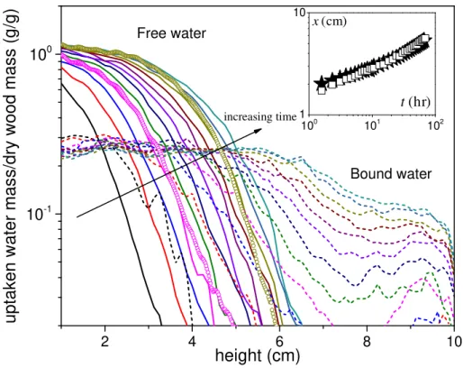
. Prior to imbibition tests, the signal intensity is calibrated by a cylinder glass tube containing a test liquid. Thus, the 1D profiles giving the amount of each type of water in thin transversal cross-sectional layers (1.25 mm thick) at different heights in the sample are15 presented in Figure 9. Note that for the sake of clarity only a few of the obtained profiles are shown in this figure. 2 4 6 8 10 10-1 100 100 101 102 10 ) (hr t ) (cm x 1
u
p
ta
k
e
n
w
a
te
r
m
a
s
s
/d
ry
w
o
o
d
m
a
s
s
(
g
/g
)
height (cm)
Free water Bound water increasing timeFigure 9 : Distribution of absorbed free water (solid lines) and bound water (short dash) contentalong the sample axis at different times: (from left to right) 3 h after first contact with water, then every 6 h. Two profiles obtained by integrating the signal at each height in the 2D images are also shown (circles). The inset shows the distance reached from bottom by the mean position of the front of the free water profiles (taken at 0.1 g/g) (stars) and the end of the uniform bound water region (squares) (the uncertainty on this measurement is ± 1.25 mm).
The free water profiles appear as a curve with approximately a given shape and simply translated towards larger distance with time (see Figure 9). It is instructive to compare these profiles with the apparent concentration distribution along the sample axis by integrating the signal obtained in the 2D images, in each elementary transversal cross-section (see Figure 9). Good consistency between the 1D profiles and those deduced from imaging was found, which confirms that the 2D images essentially show the free water distribution in the sample. Moreover, this suggests that the shape of the 1D profiles is essentially determined by the heterogeneity of the pore size distribution in different growth-rings. It is nevertheless possible that the progression in each growth-ring somewhat fluctuates in time but on average these variations would tend to balance, leading to an apparently constant shape for the 1D profiles in Figure 9.
An additional remarkable trend appears here: free water can reach most fiber lumens although the current observations show that the fibers are poorly connected (see Figure 1). As observed by Bonner and Thomas (1972) in yellow poplar, the small size and numbers of the vessel-to-fiber pits substantially reduce the effectiveness of free liquid flow. However, if the liquid flow through such pits was possible and significant, similar results should be obtained for both water and oil. Looking at the evolution of the MRI liquid distribution in time, it is seen that this is not consistent with the data (see Figure 7): oil quickly fills the volume of vessels, leading to homogenous profiles below 7 cm within 27 hours, whereas within a much shorter time water invades the vessels and appears in the fibers (the first profile of free water shown at 3h in Figure 7 already exceeds the maximum mass 0.6 g/g for oil). If there was a direct path for liquid flow into fiber lumens, and then a significant fraction of liquid is thus absorbed, then
16 there is no reason to see such different behaviors between water and oil (since oil wets well wood, as observed from global imbibition curve).
This implies that water can move through the cell walls and then appear at the fiber walls by another means. Such an effect is in fact expected: it was shown that even in the hygroscopic domain below the FSP (but close to it) some free liquid water already exists (Almeida et al. 2007) along the fiber walls. Then, more water would be progressively transported by diffusion in cell walls towards fiber lumens and finally invade them. Under these conditions the fibers close to the free water available in the vessels are the most rapidly invaded, as the moisture content (inversely proportional to the square of distance) is the largest. This implies that the invasion of the fibers by free water is more or less perpendicular to the invasion of the vessels by free water.
Let us now analyze bound water profiles. As explained above, they may not be quantitatively interpreted in terms of the total bound water amount stored at some position from the beginning of the test. Indeed, the bound water being initially present in the sample (at 53% RH) does not provide a visible NMR signal with the current sequence (see Section on NMR relaxometry), as its relaxation time is too small. It is only when sufficient water is added in the cell walls that all the bound water (i.e. initial + added) present may become visible. More precisely, beyond that critical value of bound water amount, the NMR signal increases first much faster than the concentration increase, and then increases more or less proportionally to it. This effect nevertheless does not affect the analysis of bound water dynamics since, for the sample initially at 53% RH, as a first approximation, it can be considered that a signal appears just when new bound water has been formed, and then the signal increases with the bound water amount. Finally, the present data can be interpreted qualitatively.
It appears that bound water progresses more rapidly than free water: after some time, bound water is clearly visible significantly ahead of the front of free water, associated with the vertical drop in a logarithmic scale (see Figure 9). More precisely there is a gradient of bound water concentration only beyond the region where free water exists. In order to clarify this, the evolution of the position of the beginning of curvature in the bound water profile (end of the plateau for apparent saturation of bound water) is compared with the position of the free water front. It is seen that the advance of free water coincides with the saturation of cell walls with bound water (see inset of Figure 9). It is deduced that bound water advances partly on its own well ahead of the free water region, and free water exists only where the cell walls are saturated with bound water. This is in agreement with recent observations by Gezici-Koç et al. (2017) on oak and teak, but no direct distributions of the two water components were observed in their work. Since all the initial analysis showed that the free water does not advance spontaneously due to capillary effects, it is then concluded that the bound water propagation might more or less govern the free water progression, or free water is taken up by the cell walls faster than being moved up under capillary suction. This point will be discussed further below. It was checked that qualitatively similar results, i.e. with the same major qualitative characteristics as described above, were obtained for sample initially at equilibrium at different RH values in the range 0-97%, even if the variations in bound water during imbibition are not well observed for very large RH (see Appendix D in ESM).
Deformations and bound water dynamics
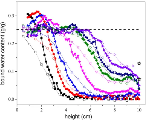
It is also interesting to look at the relationship of these transfers with the sample deformations. The present deformation measurements allow determining, for each level along the sample axis, the equivalent water volume associated with sample swelling. First of all, independent measurements showed that in the hygroscopic domain, the adsorbed water mass is equal to about 0.7 times the volumetric deformations (see Appendix F in ESM). Then with this linear relationship, the deformation data can be used to deduce the associated bound water content taking into account the initial MC. In Figure 10 the shape and the timing of this amount of bound water are compared with that measured by MRI which, as described above, may be approximately considered as proportional to the additional bound water amount. Itappears the shape and timing of both profiles are very similar. This demonstrates that there is a direct correspondence between the formation of bound water and the wood deformation.
17 0 2 4 6 8 10 0.0 0.1 0.2 0.3 b o u n d w a te r c o n te n t (g /g ) height (cm)
Figure 10 : Comparison of MRI bound water profiles (solid symbols) and bound water content deduced from deformation measurements (thin lines and open symbols) as a function of height in sample at different times: (from left to right) 1.4, 4.4, 8.3, 23.3, 47.4, 58.5, 70.5 hr. The dashed line shows the average saturation level of bound water in cell walls. The two star symbols at 10 cm show the absorbed bound water due to the vapor sorption when RH changes from 53 to 97% RH, at the end of 1 and 3 days, respectively.
Modelling bound water dynamics
It can be further elaborated on the transport of bound water in wood. It is often considered that the water vapor diffusion in air (
2
.
5
×
10
−5m2/s at 20°C) is a transport process of several orders of magnitudesfaster than bound water diffusion (Siau 1984), even though the latter concerns larger concentrations of water molecules, which tends to suggest that vapor sorption will be the dominant phenomenon for water transport. It appears that the original MRI measurements, allowing to directly observe free water dynamics and bound water dynamics, clearly show that in the present experiments there is in some region of the sample, a bound water diffusion process, which results in more moisture mass gain than vapor sorption.
Let us do some further analysis. During the imbibition tests the vapor density in the system approaches 100% since the system is covered by a parafilm in order to avoid evaporation. This has two important consequences: (i) vapor sorption can occur at the surface of all the cell walls of open paths in the sample; and (ii) vapor transport in the air due to the gradient of vapor density in lumens, is negligible (since there is a priori negligible gradient). In the presence of such a vapor density it is known that the amount of bound water grows in the form of an almost homogenous profile, with slight increase at the opened extremities of the sample (Hameury and Sterley 2006; Frandsen et al. 2007; Dvinskikh et al. 2011). The rate of sorption under such conditions is a useful information: the mass evolution in time of a small sample (2×2×2 cm3) placed at 97% RH was measured (see Appendix F in ESM). It appears that the
timing of increase of the bound water (either measured from deformation or estimated from MRI, see Figure 10) corresponds approximately to the timing of increase of the plateau of bound water observed around the top of the sample (see Figure 10). It is deduced that, as a first approximation, in the absence of liquid water penetrating the wood sample, the bound water profile in the sample placed at about 100%
18 RH would be a plateau with a level increasing like the bound water plateau observed around the sample top in the current tests. This means that in this region the impact of liquid imbibition from the sample bottom is not significant.
On the contrary, the rest of the bound water profiles, i.e. say below 8 cm, where the profiles reach the saturation value early during the test, or progressively decrease from this saturation plateau towards the final plateau (which is situated at a very low level over the first 20 hours) (see Figure 10), cannot be simply explained by the presence of vapor and possible sorption, which leads to a smaller water content increase. Since in addition these regions of large bound water amount are situated farther than the front of liquid water, it is deduced that the only possible explanation is that the liquid water in contact with the wood is adsorbed in it and diffuses longitudinally as bound water through the sample, towards the sample top.
It is assumed that there is a significant amount of bound water transport in the wood sample essentially in the form of a longitudinal transport through vessel and fiber walls. Bound water transport through cell walls can occur as a result of the gradient of chemical potential which, as a first approximation, may be considered to be proportional to the bound water fraction
n
(i.e. ratio of the amount of adsorbed water to the maximum possible amount). Then, the water fraction in the cell walls along the axisx
follows a standard diffusion equation: ∂n ∂t=D∂2n ∂x2 with D the diffusion coefficient of bound water considered as constant. In this study the boundary conditions correspond to those for a diffusion between two planes situated at x=l =0 and x=10 cm with the initial condition n(x>0)=0, the concentration at x = 0 fixed at constant value n=1 and a condition of no flux through the plane
cm 10
=
x . Under such conditions the aspect of the concentration profiles in time (Crank 1975) is
qualitatively similar to those observed for bound water beyond the saturated region (see Figure 11), i.e. with first a fast decrease of n eventually followed by a slow decrease at large distance from the front. However, a critical result from the present data, not predicted by such a simple model, is that the size (
l) of the saturated region also significantly grows (see Figure 11), which means that the distance
between the two boundaries decreases. This effect can be taken into account by imposing a diffusion from a saturated region whose front is advancing in time (according to the present observations). It is seen that this approach makes it possible to globally well represent the trends observed in these data (see Figure 11) and to obtain a rough estimate of the diffusion coefficient of bound water in cell walls, i.e.
-1 2 9 s m 10 8 . 5 × − =
D . This value is at the same magnitude as those reported before (Siau 1995;
Krabbenhoft 2003; Olek et al. 2005; Mannes et al. 2009).
Such a model for describing the phenomenon must be seen as a simplistic approach since it assumes a simple longitudinal structure of the different cell wall types, and a uniform and constant diffusion coefficient at any point in this structure, whatever the current bound water concentration. Moreover, the comparison of the model predictions with the present data is also very approximate since the measurements do not allow observing bound water below some critical concentration (see above). In order to somewhat compensate this effect for the comparison, in the model n=0 as the initial condition in the sample. Moreover, this model neglects the bound water that could be adsorbed from the vapor in the air. Nevertheless, the bound water plateau at the sample top, which was considered as that which would be obtained under purely hygroscopic conditions (see above), is finally also predicted by this simple diffusion model, but this may be explained by the fact that the model fitting is done over the whole set of profiles without specific consideration for these plateaus. A last effect also precludes a relevant detailed comparison of the model with measurements: the heterogeneity of the wood structure leading to a heterogeneous distribution of the penetration (see Figure 8), which implies that the shape of the measured 1D bound water profiles is partly altered by this effect. Nevertheless, there are qualitative trends in the measured bound water profiles which are negligibly affected by these problems and reflect the major characteristics of the process: the timing of the bound water advance (i.e. total amount in wood as a function of time, or velocity of the front) and the shape of the profiles. This simple model represents very well the observed trends with a specific value of the diffusion coefficient. Moreover, if it is now assumed that the whole water penetration is governed by a simple diffusion process from the sample bottom (i.e. Ω S= 2Dt), with this diffusion coefficient, an almost perfect
19 agreement with data is found (see Figure 6).This provides a straightforward quantitative demonstration that the whole water penetration in wood is governed by the diffusion in the cell walls.
A trend not predicted by the present model, is the increase of the bound water saturation plateau from the bottom. It was just artificially reproduced. A complete model should obviously predict the development of this saturation plateau. In order to get such a plateau a possibility is to have a diffusion coefficient increasing when n→1. Indeed, in that case the diffusion is faster close to the saturated front, so that
n
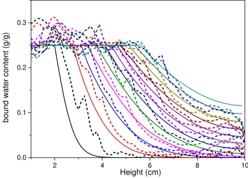
will increase faster in this region, inducing an even faster diffusion and so on. This effect, which will be more pronounced if the increase of the diffusion coefficient for n→1 is stronger, will lead to the development of a plateau whose size will progressively increase. This appears quite compatible with the observation that the diffusion coefficient increases exponentially near the FSP (Skaar 1988; Simpson and Liu 1991; Engelund et al. 2013).2 4 6 8 10 0.0 0.1 0.2 0.3 Height (cm) b o u n d w a te r c o n te n t (g /g )
Figure 11 : NMR bound water profiles (dotted lines) in the gradient region and water concentration distribution predicted by a simple diffusion model (continuous lines) from a moving front (see text) with =5.8×10⁻⁹m2.s-1
D , at different times: (from left to right) 3
h after first contact with water, then every 6 hr.
Mechanism of free water penetration
It was shown that the slow imbibition of water is likely due to the adsorption of water leading to the existence of bound water. However, this bound water does not simply transform the porous medium in such a way that its permeability is now small. Indeed, the imbibition for silicone oils, appears to be unaffected by the initial presence of bound water: within the limits of the experimental uncertainty, the imbibition curves were the same for wood samples of various initial humidities (initially either dried at 60°C, or at equilibrium with 53% RH or 97% RH). Moreover, the results, in terms of penetration dynamics, for wood samples at different initial humidities, were also similar for water imbibition, except for some slight difference in the total absorbed water amount due to the different amounts of initially adsorbed bound water. This means that, to slow down the imbibition rate of water, there is some effect occurring as a result of the interaction between the bound water either pre-existing or formed during the test, and the free water in contact with wood (at least at the sample bottom).
Considering that bound water advances beyond free water in the longitudinal direction it can finally be assumed that, in contrast to a liquid not hygroscopically adsorbed whose imbibition is governed by
20 standard capillary and viscous effects, the dynamics of water penetration is governed by bound water propagation dynamics. The ultimate question is now the origin of the slow penetration of free water in vessels. A fundamental aspect is that this phenomenon occurs at any time scale (and thus any length scale) as proved by the constant dynamics (square root of time) found for imbibition over all ranges of times. This in particular means that the physical effects at the origin of these processes occur as soon as the very first water volume enters a wood sample, i.e. at a very local scale.
There is undoubtedly a mechanism which precludes a progression of the water by capillarity through the vessels. Since this progression is driven by the wetting of the wood cell walls, this means that this wetting would be affected by the water adsorption in cell walls. Capillary action is reduced or even naturalized when adsorption occurs around the contact line of the three phases: air-water-cell wall. In parallel, when a vessel wall is saturated, some free water will appear in the neighboring fiber lumens. In addition, some water adsorbed in the cell walls will be transported longitudinally. As a consequence, the free water contained in the vessels will advance only when, just above its free surface, the wall is saturated with bound water. Then a good wetting of the wall and the impact of standard capillary effects are restored. But the corresponding progression is again stopped as soon as the liquid film reaches a region of unsaturated walls or fibers, and so on. In fact, the enchainment of these processes is likely continuous. This process in particular explains that, despite its very slow progression liquid water can still climb at a significant height, which is essentially governed by standard capillary effects (i.e. good wetting of vessel walls).
Conclusion
It was shown that spontaneous water imbibition in wood is several orders of magnitude slower than expected from standard Washburn capillary imbibition: the extremely slow dynamics suggests an angle of contact very close to π 2, while the large heights reached lead to a rather good wetting. Through various experiments under different conditions along with direct observations of the bound and free water dynamics, it was deduced that this contradiction is explained by the adsorption of bound water in cell walls, maybe a combination of vapor sorption and adsorption directly from bulk liquid. When cell walls are saturated with bound water, standard wetting can take place and free water can advance through the vessels. Thus, the dynamics of imbibition in wood appears to be mainly governed by the longitudinal progression of bound water in the sample. The position of the free water front in time is fixed by the end of the region saturated with bound water. This shows the dramatic effect of the presence of bound water on the imbibition mechanisms.
As a consequence, measurements of wood’s intrinsic permeability from spontaneous imbibition tests with water are not relevant because, as appears from the present results, the apparent permeability in that case is strongly decreased by the interplay with bound water. However, the present results also show that for any type of liquid permeability measurement, there might be a transient stage during which water adsorption may play a significant role. This effect will become negligible as soon as the medium is saturated with bound water. This might explain the variations of permeability measurements sometimes observed with the sample length.
The results open new perspectives for a control of water imbibition due to any type of contact of wood with liquid water, and the understanding of sap transfers. Further studies will be necessary to identify whether the same mechanisms take place with softwoods.
Acknowledgements: This work has benefited from a French government grant managed by ANR within the frame of the national program Investments for the Future ANR-11-LABX-022-01.
References
21 equilibrium moisture contents. Wood Sci Technol 41:293–307. doi: 10.1007/s00226-006-0116-3 Almeida G, Leclerc S, Perré P (2008) NMR imaging of fluid pathways during drainage of softwood in
a pressure membrane chamber. Int J Multiph Flow 34:312–321. doi: 10.1016/j.ijmultiphaseflow.2007.10.009
Ball P (2014) Watching wood dry. Nat Mater 13:922. doi: 10.1038/nmat4142
Bessières J, Maurin V, George B, et al (2013) Wood-coating layer studies by X-ray imaging. Wood Sci Technol 47:853–867. doi: 10.1007/s00226-013-0546-7
Bolton AJ (1988) A reexamination of some deviations from Darcy’s Law in coniferous wood. Wood Sci Technol 22:311–322. doi: 10.1007/BF00353321
Bonner LD, Thomas RJ (1972) The ultrastructure of intercellular passageways in vessels of yellow poplar (Liriodendron tulipifera, L.) part I: Vessel pitting. Wood Sci Technol 6:196–203. doi: 10.1007/BF00351577
Bonnet M, Courtier-Murias D, Faure P, et al (2017) NMR determination of sorption isotherms in earlywood and latewood of Douglas fir. Identification of bound water components related to their local environment. Holzforschung. doi: 10.1515/hf-2016-0152
Bramhall G (1971) The validity of Darcy’s law in the axial penetration of wood. Wood Sci Technol 5:121–134.
Carrillo CA, Saloni D, Lucia LA, et al (2012) Capillary flooding of wood with microemulsions from Winsor I systems. J Colloid Interface Sci 381:171–179. doi: 10.1016/j.jcis.2012.05.032
Choat B, Cobb AR, Jansen S (2008) Structure and function of bordered pits: New discoveries and impacts on whole-plant hydraulic function. New Phytol 177:608–626. doi: 10.1111/j.1469-8137.2007.02317.x
Choo ACY, Paridah TM, Karimi A, et al (2013) Study on the longitudinal permeability of oil palm wood. Ind Eng Chem Res 52:9405–9410. doi: 10.1021/ie4009259
Chu D, Xue L, Zhang Y, et al (2016) Surface Characteristics of Poplar Wood with High- Temperature Heat Treatment : Wettability and Surface. BioResources 11:6948–6967.
Cox J, McDonald PJ, Gardiner BA (2010) A study of water exchange in wood by means of 2D NMR relaxation correlation and exchange. Holzforschung 64:259–266. doi: 10.1515/HF.2010.036 Crank J (1975) The mathematics of diffusion. Clarendon Press, Oxford
De Meijer M, Haemers S, Cobben W, Militz H (2000) Surface energy determinations of wood: Comparison of methods and wood species. Langmuir 16:9352–9359. doi: 10.1021/la001080n Desmarais G, Gilani MS, Vontobel P, et al (2016) Transport of Polar and Nonpolar Liquids in Softwood
Imaged by Neutron Radiography. Transp Porous Media 113:383–404. doi: 10.1007/s11242-016-0700-4
Dvinskikh S V., Henriksson M, Mendicino AL, et al (2011) NMR imaging study and multi-Fickian numerical simulation of moisture transfer in Norway spruce samples. Eng Struct 33:3079–3086. doi: 10.1016/j.engstruct.2011.04.011
Engelund ET, Thygesen LG, Svensson S, Hill CAS (2013) A critical discussion of the physics of wood-water interactions. Wood Sci Technol 47:141–161. doi: 10.1007/s00226-012-0514-7
Faure P, Rodts S (2008) Proton NMR relaxation as a probe for setting cement pastes. Magn Reson Imaging 26:1183–1196. doi: 10.1016/j.mri.2008.01.026
Frandsen HL, Damkilde L, Svensson S (2007) A revised multi-Fickian moisture transport model to describe non-Fickian effects in wood. Holzforschung 61:563–572. doi: 10.1515/HF.2007.085 Gezici-Koç Ö, Erich SJF, Huinink HP, et al (2017) Bound and free water distribution in wood during
water uptake and drying as measured by 1D magnetic resonance imaging. Cellulose 24:535–553. doi: 10.1007/s10570-016-1173-x
González G, Siau J (1978) Longitudinal liquid permeability of American beech and eucalyptus. Wood Sci 11:105–110.
Gruener S, Sadjadi Z, Hermes HE, et al (2012) Anomalous front broadening during spontaneous imbibition in a matrix with elongated pores. Proc Natl Acad Sci 109:10245–10250. doi: