Containment analysis incorporating boundary layer heat and mass transfer techniques

Containment Analysis Incorporating Boundary Layer

Heat and Mass Transfer Techniques

by

Brett T. Mattingly B.S., Electrical Engineering

Clarkson University, 1992 S.M., Nuclear Engineering

Massachusetts Institute of Technology, 1995 Submitted to the Department of Nuclear Engineering in Partial Fulfillment of the Requirements for the Degree of

Doctor of Philosophy in Nuclear Engineering at the

Massachusetts Institute of Technology February 1999

© 1999 Massachusetts Institute of All rights reserved.

Technology.

4

Science

Author-D atment of Nuclear Engineering

Certified by

Professor Neil E. Todreas Department of Nuclear Engineering Thesis Advisor Certified by

I

Professor Emeritus Michael J. Driscoll Department of Nuclear Engineering Thesis Reader Accepted by

Professor Lawrence M. Lidsky Chairman, Department Committee on Graduate Students Department of Nuclear Engineering

Containment Analysis Incorporating Boundary Layer Heat and Mass Transfer Techniques

by

Brett T. Mattingly

Submitted to the Department of Nuclear Engineering on February 1, 1999 in Partial Fulfillment of the Requirements for the Degree of

Doctor of Philosophy in Nuclear Engineering Abstract

A new condensation heat transfer methodology has been implemented into a coarse-mesh finite-volume computer code. This methodology combines heat transfer logic based on bulk properties with the flow representation required to capture boundary layer phenomena. Application of the methodology increases the ability of the finite-volume code to predict thermal stratification, which in certain situations depends on resolving boundary layer flow adjacent to a vertical condensing surface. To achieve this, the meshing strategy employs relatively small computational cells near the surface. This approach was originally identified by Gavrilas, who proposed a noding strategy consisting of a single narrow near-wall cell and an associated heat transfer model. These concepts are extended in the present work, in which the

boundary layer hypothesis is proposed and tested. The boundary layer hypothesis consists of: 1) utilizing

two near-wall computational cells having prescribed thicknesses; and 2) employing an appropriate

condensation model. In order to demonstrate the utility of the boundary layer hypothesis, the source code of the GOTHIC 4. ic containment analysis program was modified to include the chosen condensation model and to extend the computational algorithm to allow the condensation model to be implemented correctly. A test computational problem demonstrating stratification is presented and a proposed experiment to test code capabilities is described.

A thorough literature search was performed to assess the applicability and usefulness of the available condensation models for use in the boundary layer hypothesis. The diffusion layer model (DLM), originally proposed by Peterson, was chosen as the most appropriate model for three reasons. First, the DLM is more general and accurate than the empirical model of Uchida, which is widely used in

containment analysis. Second, a modified version of the DLM has been verified against experimental data from facilities which are representative of advanced containment designs. Third, the DLM is physically grounded in mass transfer theory, consistent with the assumption of a downward flowing boundary layer, and compatible with the formulation of the boundary layer hypothesis and most finite-volume containment codes. The physical basis allows the DLM to be useful for both BWR and PWR prototypic accident scenarios, where the noncondensable gas concentration -is low and high, respectively. A thorough analysis of the DLM was performed to compare the model qualitatively and quantitatively to

other condensation models and to experimental data covering a range of expected containment

conditions. An analysis to determine model sensitivity to changes in key properties was also performed. The results of these analyses show that the DLM is more capable than the other models studied to correctly account for the influence of air, helium, and hydrogen on the condensation process. Thesis Advisor: Dr. Neil E. Todreas

KEPCO Professor of Nuclear Engineering and Professor of Mechanical Engineering

Dedication

To my parents, Beverly and Kenneth, and my sister Jeanette, for their patience and support in this endeavor

Acknowledgements

I would like to express my sincere appreciation for the help and guidance that my thesis advisors, Professor Neil Todreas and Professor Michael Driscoll, have given me over the course of this endeavor. Working with them has been a worthwhile and enjoyable experience, both personally and professionally. Thanks to Professor Mirela Gavrilas, University of Maryland, for her friendship, guidance, and encouragement in tackling some of the subject matter in this thesis. Tom George, NAI, deserves a great deal of credit for facilitating the modifications to the GOTHIC source code. Without his timely advice and assistance the code modifications would not have been possible. Professor Peter Griffith, MIT, helped me to refine the specifications for the boundary layer hypothesis. Dr. Mark Anderson and Professor Corradini at the University of Wisconsin-Madison were instrumental in my quest to evaluate the diffusion layer condensation model. They provided information on their experimental data, computer code listings, and pre-prints of their articles on the subject. Dr. Anderson also helped significantly by participating in several lengthy exchanges to resolve technical questions concerning the derivation of some key elements of the model. Thanks especially to Jennifer deVries Gwinn, MIT, for her assistance in keeping my paychecks coming over the course of the project. Finally, thanks to Dr. David Freed, Tanya Williams, and Paul Fallon for their steadfast friendship and constant encouragement. I could not have done it without them.

The sponsorship of the work in this thesis by the U.S. Nuclear Regulatory Commission in cooperation with Idaho National Engineering and Environmental Laboratory is acknowledged

and greatly appreciated. Specific acknowledgement and thanks is given to Jim Wolf at INEEL for helping to continue the project funding in unusual circumstances.

TABLE OF CONTENTS

1. INTRODUCTION AND BACKGROUND---. ---...----... ... 16

1.1 Introduction and Reasons for this Work... ₁₆

1.2 Physicaf Phenomena in Containment Analysis...16

1.2.1 Condensation ... ... 17

1.2.2 Natural convection and steam stratification... ₁₉

1.2.3 Thermal stratification in water pools...20

1.2.4 Location of phenomena... ₂₁

1.3.1 Early empirical models... ... 22

1.3.2 Simple enhancement models....erat .e.R ... .... 23

1.3.3 Modem external surface models... 24

1.4 Review of Containment Codes... 26

1.4.1 Necessary capabilities of a containment analysis code... ... 26

1.4.2 GOTHIC ....tad... ... 28

1.4.3 RELAP5/MOD3.2 .aa ...s...a.et... ₂₉

1.4.4 G A SFL O W 1.0... .. ... --... 3 0 1.4.5 TRAC-BF/MOD1... ₃₁

1.4.6 Computer codes summary ... 31

1.5 Mass Transfer Theory... ₃₃

1.5.1 Elementary mass transfer ... 33

1.5.2 High mass transfer rate theory... ... ... 34

1.5.3 Analogies between heat, mass, and momentum transfer... 40

1.5.4 Property evaluation... ₄₅

1.6 Outline of Work Presented in this Thesis... ₄₆

2. CONDENSATION MODEL EVALUATION... ₄₇

2.1 Goals of Model Evaluation ... ₄₇

2.2 Heat Sink Modeling in Containment Analysis... ₄₇

2.2.1 Small, fast acting heat sinks ... ₄₇

2.2.2 L arge surfaces... ₄₈

2.3 Surface Orientation and Gas Mixture... ₅₀

2.3.1 Description of condensation... ₅₁

2.3.3 Experim ents of Huhtiniemi and Pernsteiner ... 53

2.3.4 Experim ents of Anderson... 54

2.3.5 Sum m ary of the effect of surface orientation ... 55

2.4 Condensation M odels Under Study ... 56

2.4.1 Anderson diffusion layer model... 56

2.4.2 Other condensation models studied... 59

2.5 Property Evaluation... 60

2.5.1 Steam properties... ₆₁

2.5.2 M olar concentration and density ... 61

2.5.3 Specific heat ... 62

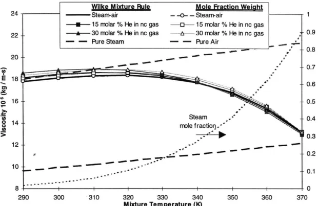
2.5.4 Viscosity ... 63

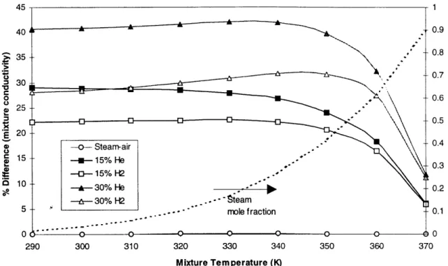
2.5.5 Therm al conductivity ... 65

2.5.6 Diffusion coefficient ... 67

2.5.7 Com parison of m ixture relations... 73

2.6 Diffusion Layer M odel Sensitivity Analysis ... 81

2.6.1 Sensitivity to specific heat... 82

2.6.2 Sensitivity to viscosity... 83

2.6.3 Sensitivity to thermal conductivity... 84

2.6.4 Sensitivity to all gases concurrently ... 85

2.6.5 Sensitivity to diffusion coefficient ... 86

2.6.6 Sensitivity to changes in gases and diffusion coefficient ... 87

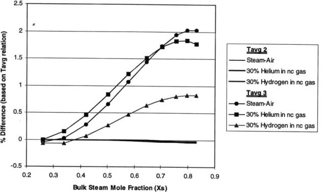
2.6.7 Sensitivity to Xs,avg and Tavg ... ... 87

2.6.8 Sensitivity to light gas concentration ... 89

2.6.9 Sum m ary of sensitivity analysis... 94

2.7 Com parison Between M odels and Data... 96

2.7.1 Steam -air mixtures ... 98

2.7.2 Helium m ixtures... 102

2.7.3 Hydrogen mixtures ... 104

2.8 Conclusions and M odel Selection... 105

3. CFD ANALYSIS OF TURBULENT BOUNDARY LAYERS ... 108

3.1 Goals of the CFD Analysis... 108

3.2 Selection and Overview of the CFX Computer Code ... 111

3.2.1 Selection of a CFD Com puter Code... 111

3.2.2 Overview of the CFX-4.2 Code ... 113

3.3 Sim ulation Specifics... 113

3.3.1 Assum ptions and Limitations... 113

3.3.2 Flow Equations and Turbulence M odels... 114

3.3.3 M odeling M ass Diffusion... 116

3.3.4 Boundary Conditions... 117

3.3.5 Convergence criteria and accuracy... 118

3.4 Benchm ark Problem ... 118

3.5 CFD Analyses... 119

4. BOUNDARY LAYER H YPOTHESIS--- --- --- --- --- --... ... ... 124

4.1 Introduction and Assum ptions... ₁₂₄

4.1.1 j ... ₁₂₄

4.1.2 Previous W ork...--... ₁₂₆

4.1.3 Proposed m ethodology ... ₁₂₈

4.2 Im plem entation into the GOTH IC code... ₁₃₄

4.3 GOTHIC Illustrative Testing and Results... ₁₃₆

4.4 A ttem pts to verify BLH against available experim ental data... 138

4.4.1 W estinghouse Large Scale Test... ₁₃₈

4.4.2 U niversity of W isconsin-M adison facility ... ₁₃₉

4.4.3 LA CE and HEDL Tests... ₁₄₀

4.5 Boundary Layer Hypothesis Sum m ary... ₁₄₀

4.5.1 U tility of the boundary layer hypothesis ... 140

4.5.2 Proposed design for an appropriate benchmark experiment ... 142

5. CONCLUSIONS AND FUTURE W ORK ... ₁₄₄

5.1 Physical Phenom ena in Containm ent Analysis ... 144

5.2 Condensation M odel Evaluation... 145

5.2.1 DLM sensitivity analysis... ₁₄₆

5.2.2 M odel com parison to experim ental data... ₁₅₀

5.2.3 Condensation m odel selection... 153

5.3 Boundary Layer Hypothesis ... ₁₅₃

5.3.1 Condensation m odel im plem entation and near-w all noding ... 154

5.4 Illustrative Test Case... ₁₅₅

5.5 Conclusions and Future W ork... ₁₅₆

REFERENCES...159

A. _{LITERATURE REVIEW OF CONDENSATION MODELS ... 166}

A . 1 Condensation on Vertical Surfaces ... ₁₆₆

A .1.1 Nusselt (1916) ... ₁₆₆

A .1.2 U chida (1965)... ₁₆₇

A .1.3 Tagam i (1965)... ₁₆₈

A .1.4 G ido and Koestel (1983) ... ₁₆₈

A .1.5 Corradini (1984-1990)... ₁₇₀

A .1.6 D ehbi (1991)... ₁₇₂

A .1.7 Peterson (1993-1996) ... ₁₇₄

A .1.8 _{M odified Peterson M odel (1997)... 176}

A _{.1.9 AP600 Sm all and Large Scale Tests ... 178}

A .2 Condensation Inside Vertical Tubes... 179

A .2.1 V ierow (1990) ... ₁₇₉

A .2.2 Siddique (1992)... ₁₇₉

A .2.3 H asanein (1994) ... ₁₈₀

A .2.4 Kuhn (1995) ... ₁₈₁

B. DERIVATION OF CONDENSATION CONDUCTIVITY ... 185

C. FLUID MECHANICS AND TURBULENCE MODELING...190

C.l Conservation Equations... 190

C. 1.1 Conservation of mass (continuity equation)... 190

C.1.2 Conservation of momentum (Navier-Stokes equations) ... 191

C.1.3 Conservation of energy (total enthalpy equation)... 192

C. 1.4 Conservation of species (mass balance for water vapor)... 193

C. 1.5 Compressible, weakly compressible, and incompressible flow ... 193

C. 1.6 Alternate forms of the fluid equations ... 194

C.2 Turbulence Modeling ... 195

C.2.1 Direct numerical simulation (DNS)... 195

C.2.2 Large eddy simulation (LES)... ₁₉₆

C.2.3 Mean flow equations (Reynolds averaging) ... 196

C.2.4 Boundary layer equations ... 199

C.2.5 Algebraic models... 202

C.2.6 One-equation models... 204

C.2.7 Two-equation models ... 206

C.2.8 Algebraic stress model (ASM)... 209

C.2.9 Differential stress model... 210

C.2.10 Turbulent heat and mass transfer... 211

C.2.11 Summary and conclusions about turbulence models... 212

D. MATHCAD WORKSHEET FOR CONDENSATION MODEL COMPARISON... 214

LIST OF FIGURES

Figure 1-1: Condensation in the presence of air on a vertical wall... 18

Figure 1-2: Stratification in a suppression pool ... 20

Figure 1-3: Location of key phenomena inside the volumes of a passive suppression pool-type containm ent system ... ₂₂

Figure 1-4: Required variables for select heat/mass transfer models... 27

Figure 1-5: Condensation from a steam-air mixture onto a liquid film ... 33

Figure 2-1: Film condensation on a horizontal surface... 51

Figure 2-2: Film condensation on a vertical surface. ... 52

Figure 2-3: Steam-air binary diffusion coefficients at one atmosphere ... 70

Figure 2-4: % Difference of steam-air binary diffusion coefficients as compared to Marrero-M ason equation at one atm osphere ... 70

Figure 2-5: Steam-helium binary diffusion coefficient at one atmosphere ... 72

Figure 2-6: Steam-hydrogen binary diffusion coefficient at one atmosphere ... 72

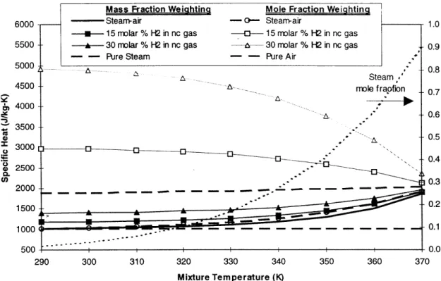
Figure 2-7: Specific heat mixture rule comparison for steam-air-helium mixtures (1 atm.) ... 74

Figure 2-8: Specific heat mixture rule comparison for steam-air-hydrogen mixtures (1 atm)...75

Figure 2-9: Error in mixture specific heat from using a mole fraction mixing rule (1 atm.)... 75

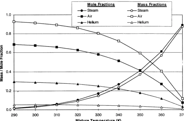
Figure 2-10: Mole and mass fractions for a 30% (molar) helium mixture at one atmosphere...76

Figure 2-11: Viscosity mixture rule comparison for steam-air-helium mixtures (1 atm.)... 77

Figure 2-12: Viscosity mixture rule comparison for steam-air-hydrogen mixtures (1 atm.) ... 77

Figure 2-13: Error in mixture viscosity from using a mole fraction mixing rule (1 atm.)...78

Figure 2-14: Conductivity mixture rule comparison for steam-air-helium mixtures (1 atm.) ... 79

Figure 2-15: Conductivity mixture rule comparison for steam-air-hydrogen mixtures ... 79

Figure 2-16: Error in mixture conductivity from using a mole fraction mixing rule (1 atm.) ... 80

Figure 2-17: DLM sensitivity to changes in mixture specific heat ... 82

Figure 2-18: DLM sensitivity to changes in mixture viscosity ... 83

Figure 2-19: DLM sensitivity to changes in mixture conductivity ... ... 84

Figure 2-20: DLM sensitivity to change in all mixture rules concurrently ... 85

Figure 2-21: DLM sensitivity to changes in diffusion coefficient ... 86

Figure 2-22: DLM predictions using logic of Anderson compared to that of Mattingly ... 87

Figure 2-23: DLM sensitivity to alternate definitions of Xs,avg compared to baseline... 88

Figure 2-24: DLM sensitivity to alternate definitions of Tavg compared to baseline ... 89

Figure 2-25: Density of gas mixtures at 1 atmosphere with helium or hydrogen present... 90

Figure 2-26: Normalized Grashof numbers of steam-air and steam-air-hydrogen mixtures AT = 10K (normalized to Grx "3 _{= 1. 154x 103, value for pure air at Tbuwk=300K)... 91}

Figure 2-27: Light gas effects on DLM predictions of Anderson and Mattingly... 92

Figure 2-28: HTC change with helium or hydrogen for different Tbulk, AT=30K... 93

Figure 2-29: Effect of hydrogen and wall temperature on total HTC ... 94

Figure 2-30: Model comparison to steam-air data from the atmospheric facility ... 98

Figure 2-31: Model comparison to steam-air data from both UW facilities (1 atm) ... 100

Figure 2-32: Suction effect / data comparison for steam-air mixtures, P = 1.5 - 3.0 Bar ... 101

Figure 2-33: Model comparison to UW pressurized steam-air data, P = 1.5 -3.0 Bar ... 101

Figure 2-35: Model comparison to UW steam-air-helium data (1 atm.) (XHe/Xnc= 0.3) ... 103

Figure 2-36: Model comparison to steam-air-helium data at P = 1.5 -4.5 Bar (XHe/Xnc= 0.3). 104 Figure 3-1: Figure 3-2: Figure 3-3: Figure 3-4: Figure 3-5: Figure 3-6: B enchm ark C FD problem ... Problem specification for CFD analysis of boundary layers ... Normalized temperature profiles for air-only convection ... Velocity profiles for air-only convection... Normalized scalar profiles for condensation... Velocity profiles for mixed convection condensation... Figure 4-1: Boundary layer cell proposed by Gavrilas [Gavrilas, 1995]... 128

Figure 4-2: Algorithm for implementing the boundary layer hypothesis into GOTHIC... 130

Figure 4-3: Velocity profiles from the integral method for laminar and turbulent natural convection boundary layers along a vertical flat plate ... 132

Figure 4-4: Temperature profiles from the integral method for laminar and turbulent natural convection boundary layers vertical flat plate ... 132

Figure 4-5: Comparison of CFD predictions to those of the integral method... 133

Figure 4-6: Illustration of boundary layer cell arrangement... 134

Figure 4-7: Schematic of test case to illustrate the utility of the boundary layer hypothesis ... 137

Figure 4-8: Steam concentration and temperature profiles predicted by GOTHIC for the test case show n in figure 4-7 ... 137

Figure 4-9: Steam concentration profiles predicted by test case with concrete walls... 138

Figure 4-10. Large Scale Test cross section... 139

Figure 4-11: Flowchart for implementing the boundary layer hypothesis ... 142

Figure 5-1: Figure 5-2: Figure 5-3: Figure 5-4: Figure 5-5: Figure 5-6: Figure 5-7: Figure 5-8: Figure 5-9: shown Condensation in the presence of air on a vertical wall... 145

Sensitivity of DLM predictions to hydrogen and helium, (Tbuk-Twa=30K)... 147

Sensitivity of DLM to wall temperature for steam-air-hydrogen mixtures ... 148

Model comparison to UW data for air-steam, (P = 1.0 Bar) ... 151

Model comparison to UW and MIT data for steam-air, (P > 1.0 Bar) ... 151

Model comparison to UW and MIT data for steam-air-helium, (P > 1.0 Bar)... 152

Details of the logic of the boundary layer hypothesis... 154

Test case to illustrate the utility of the boundary layer hypothesis... 155

Steam concentration and temperature profiles predicted by GOTHIC for the test case in F igu re 5-8 ... 156

Figure B-1: Condensation from a steam-air mixture onto a liquid film... 187 118 119 121 121 122 123

LIST OF TABLES

Table 1-1: Summary of computer code capabilities... 32

Table 1-2: Prandtl and Schmidt numbers of relevant gas mixtures ... 44

Table 1-3: Normalized Grashof numbers of relevant gas mixtures ... 45

Table 1-4: Possible definitions of the reference state to evaluate transport properties... 46

Table 2-1: Important parameters for heat sink modeling ... 50

Table 2-2: Studies on orientation, gas mixture and condensation rate... 52

Table 2-3: Specific heat (J / kg-K) comparison with reference values ... 63

Table 2-4: Viscosity (x106 kg / m-s) comparison with reference values ... 64

Table 2-5: Thermal conductivity (mW / m-K) comparison with reference values ... 66

Table 2-6: Lennard-Jones potential force constants... 68

Table 2-7: Range of conditions for DLM sensitivity analysis... 81

Table 2-8: Posible definitions for Tavg and Xs,avg... 88

Table 2-9: DLM sensitivity to changes in particular variables ... 95

Table 2-10: Recommended methodology for property evaluation in the DLM... 105

Table 2-11: Recommended Lennard-Jones force constants for DLM implementation ... 106

Table 2-12: Difference between implementation of Mattingly and Anderson... 107

Table 3-1: G oals of the CFD analysis ... 111

Table 3-2: Codes investigated for CFD analysis... 111

Table 5-1: DLM sensitivity to changes in particular variables ... 149

Table 5-2: Range of conditions for DLM comparison to experimental data ... 157

NOMENCLATURE

f

j

J

volumetric mass source rate molecular weight

absolute molar flux (scalar) absolute molar flux (vector) pressure (instantaneous) pressure (time average) turbulent Prandtl number heat flux

volumetric heat source rate universal gas constant volumetric molar source rate Turbulent Schmidt number time

mole transfer diffusion driving force mass transfer diffusion driving force heat capacity at constant pressure

gas concentration (molar density) blowing factor (suction factor)

skin friction coefficient tube diameter

binary diffusion coefficient (mass diffusivity) eddy diffusivity of momentum

eddy diffusivity of heat eddy diffusivity of mass

friction factor (Fanning or Moody) gravitational acceleration

mass transfer conductance

mass flux in direction of mean flow heat transfer coefficient

static enthalpy

specific enthalpy of vaporization total enthalpy

diffusive mass flux (scalar) diffusive mass flux (vector) diffusive molar flux (scalar) diffusive molar flux (vector) thermal conductivity

turbulent kinetic energy length of surface

mass fraction mass flux

T u,v,w U* v V vn Vn V U,V,W W x,y,z X [K] [m s] [m s] [m s] [m /s] [m /s] [m /s] [m s] [m /s] Greek symbols

cc

)=(Sc

_(pux/)

velocity vector components friction velocity

molar-average mixture velocity (scalar) molar-average mixture velocity (vector) absolute velocity of species n (scalar) absolute velocity of species n (vector) velocity vector

average velocity components mass fraction

coordinate directions mole fraction

thermal diffusivity

mass flux per unit circumference thickness

Kronecker delta

dissipation rate of turbulent kinetic energy dynamic viscosity

kinematic viscosity (momentum diffusivity) density

turbulent Prandtl number for K turbulent Prandtl number for E shear stress

specific volume

blowing or suction factor

Grashof number Jacob number Lewis number Nusselt number Prandtl number Reynolds number Schmidt number Sherwood number Stanton number

Subscripts

1 without shear stress

2 with shear stress

a,air air property avg average

b,bulk bulk steam/gas mixture property c condensation

cond condensation conv convection

e free stream quantity

fg liquid to vapor phase change

g noncondensable gas property (at gas partial pressure)

i evaluated at the condensate interface

i,j,k indices'for tensor notation

1 liquid (condensate) property

Superscripts

average value FC forced convection NC natural convection

sat water/steam saturation property ss steady state

trans transient

laminar

steam/gas mixture property radiation

steam property

(at steam partial pressure) smooth condensate film turbulent

turbulent boundary layer total

vapor (steam)

evaluated at the wall wavy condensate film la m rad s sf t tbI T V w wf

1.

INTRODUCTION AND BACKGROUND

1.1 Introduction and Reasons for this Work

The main focus of this thesis is to advance the analysis techniques which are used to evaluate and predict the performance of passive nuclear reactor containment systems. The current analysis techniques rely heavily on computerized tools to simulate phenomena such as circulation and condensation inside the containment vessel. The analyst has benefited from advances in

computer speed in recent years, making detailed, computationally intensive, simulations possible. This increased level of detail allows the modeler to resolve small changes in buoyancy or mass concentration within the containment structure. This resolution is necessary for predicting the performance of passive containment systems since most passive systems rely on buoyancy differences or other small gradients to provide the driving force for operation. However, greater detail is not the only advance needed to predict passive system performance. The models which are implemented in the computational tools must be used in a manner which is consistent with their derivation. Choosing the correct phenomenological models and properly implementing them, using the appropriate level of resolution, is the key focus of this project.

The project was performed in three stages. The first stage was a thorough review of the current state of knowledge for the phenomena encountered when predicting containment performance. As such, the first stage centers primarily around evaluation of several computer codes and different condensation models. The second stage consisted of a sensitivity study on the most appropriate condensation models identified in stage one and a careful evaluation of how to implement them properly into the tools that MIT has available to predict containment

performance. The third stage consisted of numerically studying natural convection, turbulent, condensation boundary layers and finally implementing a new condensation boundary layer model into the finite-volume computer code GOTHIC, which is used for overall containment assessments.

The remainder of this chapter gives some background for the work which is presented in the following chapters. Section 1.2 gives a description of the key physical phenomena which must be modeled in order to predict the performance of an advanced containment system with passive heat removal. Section 1.3 reviews several containment analysis codes which are currently available and lists their strengths and weaknesses. Section 1.4 gives an overview of the

condensation models available and outlines the literature review given in Appendix A. Section 1.5 gives a short review of the condensation mass transfer theory which is central to the

condensation model which is focused on in the remainder of the thesis. Finally section 1.6 gives an overview of the work presented in the remaining chapters.

1.2 Physical Phenomena in Containment Analysis

This section identifies the key phenomena that are encountered in a passive containment facility. In order to simulate the integral performance of a passive containment system, the analysis tool, usually a computer code, must predict the interaction between several different phenomena under changing conditions. The three phenomena which are most important in a passive containment system are: condensation of steam (often in the presence of a noncondensable gas); natural and

mixed convection; and stratification of liquid and vapor regions. These three phenomena are discussed in more detail below.

1.2.1 Condensation

Condensation is the primary means of removing heat and limiting the pressure increase following a loss of coolant accident (LOCA) inside any nuclear reactor containment vessel. Historically, suppression pools, fan coolers, and water sprays have been used to rapidly condense water vapor and reduce the overall containment pressure and temperature. A suppression pool, while a feature in many traditional containment designs, is also an example of a passive system that performs a primary function in limiting pressure rise. The suppression pool does not require power to function and is a fast acting and highly effective method of condensing a large amount of steam in a short period of time. However, a traditional suppression pool loses effectiveness after the initial blowdown period, when the pressure difference between the drywell and the wetwell becomes small. New designs must be employed to keep passive systems like a suppression pool functioning in order to control the long-term containment pressure in the absence of active heat removal systems.

During and after the blowdown period, condensation on heat sinks inside the containment vessel plays a key role in helping to limit the pressure in a passive containment system. In the short-term (t < 500 seconds) fast acting heat sinks are very effective as cool surfaces for condensation. However, these fast acting heat sinks, which are mostly steel components, become saturated quickly, and only the large steel and concrete containment structures and in-containment water pools remain as inherent surfaces for condensation in the long term. Since decay heat continues to be released into the containment following the initial blowdown, long-term heat removal is necessary to reduce the containment pressure. This heat removal is usually accomplished by a combination of methods. The passive heat capacity of the containment structures are important contributors, and in addition several containment concepts have long-term passive heat removal systems that are designed to condense water vapor.

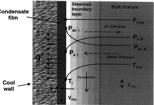
Modeling condensation on surfaces and in passive systems is not always a straightforward task. Two complications arise immediately. The first is the presence of a noncondensable gas, the second is the geometric layout of the containment and the heat sink surfaces. A noncondensable gas acts to severely hinder the condensation process. Whereas condensation of pure steam is generally limited by the resistance to heat transfer of the condensate film, condensation in the presence of a noncondensable gas is diffusion limited. While the steam/gas mixture moves toward the cool surface, only the steam changes phase to liquid, leaving the noncondensable gas to collect at the interface. This gas buildup forms a diffusion boundary layer. In order for the steam to condense, it must first diffuse through this noncondensable boundary layer, causing a decrease in the condensation rate. Because the noncondensable gas builds up at the interface, a very small concentration of noncondensable gas in the bulk atmosphere can cause a severe decrease in condensation rate.

Condensate film

Cool T

wall

VfJ

Figure 1-1: Condensation in the presence of air on a vertical wall

Adapted from [Collier, 1981]

Figure 1-1 illustrates the situation for a flat vertical wall. At the outer limits of the boundary layer, the partial pressures of steam and air are in equilibrium with the local atmospheric conditions. As one moves through the boundary layer toward the condensate film, the steam partial pressure decreases while the air partial pressure increases. At steady state, the partial pressure of air at the interface reaches an equilibrium condition where the amount of air being carried to the interface by the incoming steam-air mixture exactly equals the amount of air diffusing away. The condensation rate is limited by the amount of steam that can diffuse or convect through the air layer. Steam diffusion is driven by the steam partial pressure gradient between the bulk conditions and the interface, whereas steam convection is a result of fluid motion within the boundary layer. A suitable condensation model which represents these

phenomena must be employed to accurately predict the condensation rate on large surfaces inside the containment. Choosing such a model is the basis for the condensation literature review which is presented in Appendix A.

Further complications for modeling condensation arise from the complex geometries involved. The containment vessel houses pumps, ladders, walkways, pools, and many other structures that act as heat sinks following a LOCA. Condensation inside tubes in a passive condenser is also different from condensation on a surface in contact with a large atmosphere. As gas flows through the tube, steam can not diffuse in from a near-infinite bulk mixture region as is the case for condensation on walls. Thus, the entire mixture inside the tube (not just the boundary layer) becomes depleted of steam. Ideally, the computer code used to analyze the containment response would be able to represent the condensation on each structure taking into account the different geometric influences on airflow and condensation rate. When trying to predict the long-term pressure response of a containment system, this approach is far too cumbersome for efficient analysis, and fortunately can be avoided based on rational arguments. Section 2.2 discusses this problem in detail.

1.2.2 Natural convection and steam stratifcation

In traditional containment designs, active systems such as water sprays and fan coolers force the atmosphere inside the containment to remain relatively well mixed following a LOCA. A well mixed atmosphere simplifies a containment performance analysis by allowing the analyst to treat the atmosphere as a single homogenized region. With a homogenized atmosphere, all heat sinks

and containment surfaces can be assumed to be in contact with a vapor mixture that is at a uniform temperature and steam concentration. When the assumption of a well mixed atmosphere is valid, the containment pressure response can usually be evaluated using analytical methods or

simple computer programs based on a lumped parameter modeling approach. When this assumption is not valid, a more complex modeling approach is necessary.

In many passive containment systems, the steam atmosphere can not, a priori, be assumed well mixed. Immediately following a LOCA, the atmosphere will be relatively homogenous as a result of the violent mixing which occurs during the blowdown. However, after the blowdown has ceased and steam begins to condense on structures and passive systems begin to operate, the atmosphere may begin to stratify. In the case of the boiling water reactor SBWR design, the upper drywell and lower drywell are connected through a relatively small opening. In addition, the lower drywell is a "dead end" volume. The result is that during the blowdown the gas in the upper drywell is forced into the suppression pool, while the gas in the lower drywell is merely compressed by incoming steam. Thus at the end of the blowdown phase, the drywell atmosphere is not uniformly mixed in all areas. A similar situation exists in the pressurized water reactor AP-600 design. The below-operating-deck rooms in the containment are somewhat isolated from the above-deck region, and some do not participate in the violent mixing that occurs. The high concentrations of noncondensable gas in these regions causes the gas to diffuse back into the steam-rich regions. Thus the gas/steam mixture is not uniform once this later mixing begins to occur.

Many of the structures that act as passive heat sinks are located in small rooms within the containment building. After a LOCA the steam concentration in these rooms may be different from the concentration in the bulk atmosphere due to a higher condensation rate. Most

importantly, however, is the approach used in representing the difference in steam concentration that exists within the bulk atmosphere of the drywell region. Steam is generally more buoyant than air, thus in the absence of strong mixing forces one would expect a steam-rich region to develop near the top of the containment vessel, with an air-rich region in the lower containment. Clearly, accurate modeling of condensation on the heat sinks in these regions will be depend on the local steam concentration, and treating the atmosphere as one homogenized region could introduce significant errors into the analysis. Also, for designs which use passive condensers, such as the SBWR, it is important to know the steam-air concentrations at the condenser inlets in order to calculate the correct rate of heat removal by the condenser units.

All of these factors point to the need for modeling natural convection within the containment atmosphere. Natural convection is a process in which buoyancy provides the forces which cause fluid motion. Correctly modeling this fluid motion is essential if one wishes to predict

stratification within the containment and the correct heat transfer rates on containment surfaces. Condensation on walls will cause a cooling effect that induces the down-flow of the steam-air

mixture at the wall. This causes shear induced mixing forces in the surrounding fluid.

Conversely, a hot steam plume will rise, entraining other fluid with it, causing a second type of mixing motion. Modeling these natural convection processes requires a relatively fine

computational mesh within the open containment space and a computer code which can calculate two- or three-dimensional flow within a region. When the natural convection forces can be modeled by the computer code, phenomena such as stratification and location-specific heat transfer are amenable to prediction.

1.2.3 Thermal stratifcation in water pools

Stratification of steam within the containment atmosphere was discussed above in the section on natural convection. However, thermal stratification within a water pool is also a key

phenomenon within a passive containment design. The two most important pools considered here are the suppression pool and the passive cooling condenser pool. A suppression pool generally has several vents which allow steam from the drywell to enter the suppression pool at different elevations. Figure 1-2 shows a typical suppression pool configuration.

PCCS Noncondensable vent

Stratification = a "total + Pair f (Twater)

Drywell vents

Figure 1-2: Stratification in a suppression pool

For a large break LOCA, the pressure difference between the drywell and suppression pool will be sufficient that steam will be forced through all three vertical vent openings into the pool. This will cause the pool to become relatively well mixed. For a small break LOCA, the pressure rise in the drywell may only be sufficient to force steam through the top vertical vent opening. In this situation, it is expected that the suppression pool will stratify. Stratification in a suppression pool caused by a low steam flow rate was the subject of experimental investigation in Japan [Kataoka,

1992]. Kataoka showed that stratification occurs just below the steam release point and is quite well defined. The water above the stratification layer is uniformly warm, whereas the water below the stratification layer is uniformly cool. The stratification layer moves downward via conduction only. This phenomenon essentially reduces the amount of water which acts in the steam suppression process, thereby reducing the total heat capacity available for safety functions.

A more important consequence of this type of stratification can occur in the suppression pool of a SBWR type reactor, where the passive containment cooling system (PCCS) vents

noncondensable gases from the passive condensers. This arrangement is also shown in Figure 1-2. In the case where the PCCS condensers are not able to condense all of the steam, there will be some steam which gets vented to the suppression pool along with the noncondensable gases. This steam will then condense in the suppression pool and cause heating of the top layer of water which is above the PCCS vent tube outlet. Since this steam/noncondensable mixture has a very low velocity, no significant mixing will result and a stratification layer is expected to form. The problem associated with this is the wetwell gas space pressure. The wetwell gas pressure is a strong function of the temperature of the water surface, since the saturation pressure of water vapor and the temperature (and thus pressure) of the noncondensable gas are closely related to the water surface temperature. A significant rise in the water surface temperature will cause a corresponding rise in the wetwell gas space pressure, and thus a rise in the pressure of the

drywell. This phenomenon opposes the desired effect of long-term pressure reduction as a result of PCCS operation and should be captured in a containment performance analysis.

A second type of water pool that may become stratified during a LOCA is the PCCS pool in an advanced containment design. The passive condensers are submerged in a pool of water which acts as the secondary side heat sink. In most designs steam from the containment condenses on the tube inner surface and the heat released from condensation causes the water in the pool to boil. Since the steam/air mixture enters the condensers from the top, the highest rate of

condensation occurs at the tops of the tubes. Thus the highest rate of heat transfer to the liquid is also near the top of the pool. The water at the top of the pool is at a lower hydrostatic pressure, and thus boils more rapidly than the water further down in the pool. These effects may combine to produce pool stratification, especially in the absence of vigorous boiling, which may be the case late in the transient. The effects of varying pool temperature on the PCCS system may be a significant factor in determining the overall performance of the containment system.

The ability of a computer code to predict pool stratification is directly related to how it models convection and fluid motion. A code which is able to predict natural convection in the gaseous

atmosphere, should be able to predict stratification in water pools, if the code is a general two-phase code. Because liquid water has a significant density, a haphazard noding scheme can induce spurious mixing currents and force mixing in cases where stratification should be observed. Attention should be paid to the specific computer code instructions on how to avoid such numerical problems. Although pool modeling has been identified as a key parameter in containment analysis, this topic is not be covered in the remainder of the thesis. Instead, the focus is on the problem of condensation and circulation within the vapor region, which is considered to be more urgent.

1.2.4 Location qf phenomena

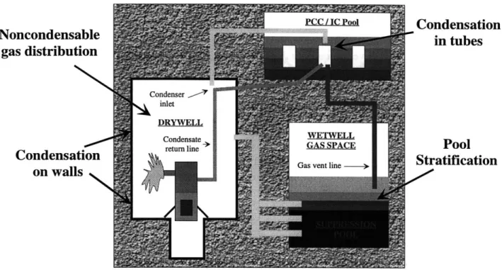
The three basic phenomena discussed in this section have been determined to be of primary importance when evaluating the performance of a passive containment system. Figure 1-3 shows a simplified layout of a suppression pool-type advanced reactor containment system with the locations of the key phenomena indicated. The most important phenomenon is condensation in the presence of a noncondensable gas which occurs in the condenser tubes and on passive heat

sinks such as walls, floors, and steel components. Section 1.4 presents an overview of the different condensation models that are available for use in analyses of this type.

Noncondensable gas distribution Condensation on walls Condensation in tubes Pool Stratification

Figure 1-3: Location of key phenomena inside the volumes of a passive suppression pool-type containment system

1.3 Summary of Condensation Literature Review

A large part of the background work for this thesis consisted of a thorough literature review of condensation models for both internal and external surfaces. Since a containment atmosphere nearly always has noncondensable gases present, the literature review focused on condensation

with this condition. There have been many models developed recently for both condensation on large surfaces and inside tubes. The structure of the models ranges from purely theoretical to purely empirical, with several somewhere in between. Not all of the models are easily

implemented into some of the less sophisticated, early computer codes. However, advances in computer analysis techniques in the last decade have made implementation of complex models much easier. Appendix A gives a review of the most relevant condensation work published in the last fifteen years, and the reader is referred to it for an in-depth look at each of the models. This section summarizes the results of the literature review and highlights which models will be the focus for the remainder of the thesis. Most of the discussion past this point will be concerned with condensation on large external surfaces as opposed to condensation inside tubes.

1.3.1 Early empirical models

The most widely known empirical models for condensation inside a containment building are those of Uchida and Tagami [Uchida, 1965; Tagami, 1965]. These models have been used for many years as the standard tool for predicting inside containment condensation rates. Uchida and

Tagami performed condensation experiments using a small cylinder in a vessel which was initially filled with one atmosphere of a noncondensable gas. The gases studied were air,

nitrogen, and argon. During the Uchida tests, the cylinder surface temperature was held constant while the vessel was filled with steam until a steady state pressure was reached. A curve fit to the Uchida steady state data results in the expression below which is often referred to as the Uchida model:

h = 379 (mg /m, )-0707 (W / m2 _{K) (1.1)}

Tagami gathered transient data and produced a set of equations which can be used to describe the rate of heat transfer as a function of time. The Tagami method for predicting heat transfer is very crude and should be used only when performing a cursory, lumped parameter study. The Tagami data, however, have been used for comparison by many researchers who have since developed more advanced models. The Tagami model is given as equations (A.4 -A.5) in Appendix A. The Uchida (and Tagami) model does not take into account any local parameters, but is instead based solely on the average bulk steam and air mass fractions. This type of model is well suited to lumped parameter computer analysis, and has historically been viewed as conservative. The paper by Gido & Koestel noted that the small scale experiments produced laminar condensation data which consistently under-predicted condensation data from large surfaces, which are in the turbulent regime [Gido, 1983].' However, recently Peterson showed that the Uchida model only works well for situations that match those in which the data were taken - i.e. a noncondensable gas partial pressure of about one atmosphere [Peterson, 1996]. The theoretical study showed that the Uchida model can over-predict the rate of condensation heat transfer if the partial pressure of noncondensable gas in the containment is significantly below one atmosphere. This situation often arises in the drywell of a suppression pool-type containment, where most of the

noncondensable gases are purged to the wetwell during the blowdown. This situation can also occur in sub-atmospheric containment buildings and in individual compartments of a

containment that may be purged of their noncondensables for some reason. These two

shortcomings have basically meant that the Uchida model has outlived its usefulness in modem containment analysis, except as a simple first approximation tool.

1.3.2 SimIe enhancement models

One of the simplest types of theoretical condensation models is based on a heat transfer coefficient for dry air convection multiplied by an enhancement factor for condensation. This type of approach is often used in analyses of air conditioning or dehumidifier systems. An expression for the mass transfer coefficient can be written [Research and Education Association,

1984]:

h Sc 2/3 h I

hD = P"(r - PC " 2l 3 (1.2)

pci, Pr pc, Le~

Gido and Koestel proposed their own condensation model which is a combination of natural and forced convection heat transfer expressions (see Appendix A for details).

where the total heat transfer is given by:

q"= h .AT +hD Achf (1.3)

Another such model is given by [Threlkeld, 1970]:

C + Cp(water) +h

[hPiair

= hapa (1.4)

Cip(air)

where p is the mass of water vapor per unit mass of air. These models are both based on the heat and mass transfer analogy, but are limited in their range of applicability to instances where the water vapor partial pressure is small. These models are suitable for the applications cited above which generally have air temperatures less than 40'C, a total pressure of about one

atmosphere, and a condensing surface below 200C. When one attempts to apply these models to other conditiorts, they can incur large errors. Since the atmosphere in a post-LOCA containment building generally has a vapor partial pressure equal to or exceeding those of the noncondensable gases, this type of model is not adequate.

1.3.3 Modern external surface models

More recent theoretical models for external surface condensation have emerged which are capable of describing the processes of condensation and convection based on local parameters. This type of model is necessary in the analyses of an advanced containment design because the atmosphere may not be well mixed. These new models treat heat transfer through the condensate film and through the gas boundary layer as two distinct processes occurring in series. Heat transfer through the boundary layer is further treated as three parallel processes: convection (or sensible heat transfer); condensation (or latent heat transfer that accompanies mass transfer); and radiation. Equations (1.5) and (1.6) describe this process2

1 1 1 (1.5)

h- h" g'as

hgas =khon+ hn+ hrad (1.6)

Researchers have debated back and forth whether modeling of the condensate film is necessary for condensation in the presence of a noncondensable gas because the resistance to heat transfer from the boundary layer is much greater than that from the film. However, it has been argued that for high vapor velocities, or low noncondensable gas concentrations, the heat transfer

coefficient in the boundary layer can approach that of the condensate film [Kim, 1990]. It is also necessary to include the condensate film if one wishes to have a general condensation model which can be used in a computer code to describe condensation under any circumstances, which

is a desirable trait in this author's opinion.

2 The radiation term in equation (1.3) is usually dropped because the atmospheric temperature in most containment

Two researchers who have made recent advances in this field are Corradini and Peterson (see Appendix A for details of their work). Corradini assumed that condensation boundary layers on large surfaces are turbulent, and using the heat/mass transfer analogy and empirical relations for turbulent quantities devised a method to predict condensation under such conditions [Corradini, 1984]. The Corradini model was later extended to include waviness effects from the condensate film [Kim, 1990]. The Corradini approach requires knowledge of steam concentrations both inside and outside the boundary layer, and iteration on the condensate film temperature to match the heat transfer rate through the film with that through the boundary layer. Later Peterson derived an expression called the condensation conductivity, which allows the mass transfer process, which is driven by concentration gradients, to be expressed in terms of saturation temperatures3 [Peterson, 1993]. Then by invoking the heat and mass transfer analogy, a simple expression for treating heat transfer through the gas boundary layer was developed. Peterson's model also requires iteration on the condensate film temperature, but is applicable to internal and external condensation since the model is general and based on choosing an appropriate Nusselt number for the.particular situation being studied.

Both of these models are fundamentally derived from theory, instead of being purely empirical, which makes them more robust and applicable to a wider range of conditions than models such as Uchida. The model which is used throughout the remainder of this thesis is the Peterson model, which has a few extensions by Anderson to treat high mass transfer rates [Anderson,

1998] (also see Appendix A). The modified Peterson model is termed the diffusion layer model or DLM, and obeys the following equations:

hon, =km Nux (1.7) hcond - Sh E (1.8)

x x h cM2_{D 1-X} kcond =

(

0-X

j=s

llXgj,/g,j]

The DLM is in a form which can easily be implemented into a computer code for performing containment analysis. This model is also able to predict local values of the heat transfer

coefficient, which makes it applicable for studies where conditions may change drastically over the length of a single surface. This type of flexibility is desirable for a model to be used in analyzing advanced containment systems. This model is studied extensively in Chapter 2 of this thesis. Several other condensation models were identified as being relevant during the literature review. Appendix A presents these additional models in detail, and discusses their strengths and weaknesses. There is also a section of Appendix A dedicated to condensation inside tubes, which is not a topic that will be discussed frequently in this thesis, although it is relevant to many types of passive containment cooling systems.

1.4 Review of Containment Codes

Several computer codes are currently available for the analysis of nuclear reactor containment systems. This section provides a brief overview of four major codes and presents an evaluation based on the ability of each code to simulate key phenomena in the containment system. The key physical phenomena which occur in passive containment systems were identified in section 1.2. Prediction of these phenomena often requires that a code have several distinct capabilities. These capabilities are briefly described next.

1.4.1 Necessary capabilities of a containment analysis code

The key physical phenomena that a computer code must ideally be able to simulate in the analysis of a passive containment system are:

* Condensation in the presence of noncondensable gases; " Natural (buoyancy induced) convection and mixing; " Stratification in liquid or gas volumes.

The first, condensation in the presence of a noncondensable gas, requires that the code be able to calculate the variables which are needed for the particular heat and mass transfer models. This usually requires the calculation of several parameters near a wall or other boundary as well as the ability to track a noncondensable gas mixture separately from the steam phase. Figure 1-4 shows the variables which a code must calculate in order to use the Uchida correlation, the Gido & Koestel correlations, or the Peterson diffusion layer model (DLM). Most codes calculate

variables which are necessary for the Uchida and Gido & Koestel models. However, many codes do not calculate the liquid film interface temperature or the steam partial pressure at the interface. These quantities are necessary for the DLM.

A second and closely related process that a code must be able to simulate is natural convection. This requires that the code be able to predict buoyancy-induced driving forces for fluid motion. For the proper prediction of these forces, a code should have three-dimensional capability. The buoyancy-induced forces of free or mixed convection are localized phenomena and can not necessarily be treated symmetrically. Imposing a one-dimensional or two-dimensional4 _solution scheme on a containment problem is forcing the problem to be treated symmetrically. Symmetry can sometimes be used to simplify a containment analysis, but in many cases it is known a priori that the problem will be asymmetric (i.e. for an off-center steam release.) Similarly, a multi-dimensional velocity and momentum solution allows for stratification to develop in different regions of the containment atmosphere. Predicting stratification is essential to being able to predict real situations. Also, the possibility of stratification indicates that heat transfer and condensation should be calculated on a local basis, not on an average basis over large surfaces.

4 _{An example of a two-dimensional solution scheme would be a cylindrical coordinate representation of a cylindrical}

containment volume with radial divisions but no divisions in the azimuthal direction. Such a treatment models the problem as a set of concentric annuli, where the flow in each annulus is assumed homogenous. Such a situation may be envisioned for flow in pipes, but is not a realistic model for a large containment volume because of

non-symmetric break release locations, heat sink distributions, and the large distances between supposedly homogenous regions.

PetersonP (DLM)

Uchida and Gido & Koestel

* Gido & Koestel only

Figure 1-4: Required variables for select heat/mass transfer models

This local heat transfer calculation requires the use of local heat transfer models and computer code logic which are set up to perform this function. Many older computer schemes do not contain this flexibility (e.g.,GOTHIC version 3.4e and earlier).

The previous paragraph necessitates a discussion of the basic distinction between a "lumped parameter" (LP) computational scheme and a "distributed parameter" (DP) computational scheme. In a LP analysis, the containment is usually represented by relatively large

computational volumes. These volumes are assumed to be homogenous and all fluid properties (e.g. temperature & steam partial pressure) are calculated on a volume-average basis. No fluid velocities are calculated within a LP computational cell. Velocities induced by the net change of mass between volumes is modeled as flowing through a one-dimensional junction (pipe) only and is a result of pressure difference between the volumes. By definition, local heat and mass transfer correlations cannot be used in LP studies, only average heat transfer relations can be used. It is also an assumption that any liquid present in the volume is in a pool at the bottom. Thus a condensate liquid film on a vertical wall cannot be modeled within a LP volume. On the other hand, DP modeling refers to a situation where a single large volume is discretized into smaller subvolumes. Each subvolume is referred to as a cell. Fluid properties are still calculated on a volume average basis, but within each subvolume. Fluid velocities do exist within subvolumes and velocity directional components are calculated as the average of the velocities on opposing faces (boundaries) between cells. Each cell has six faces, thus there are velocity components in all three dimensions. The basic distinction between a computational model with a large number of LP volumes connected together and one with a single DP volume subdivided into smaller cells, is the ability to predict three-dimensional velocity and momentum transfer in the DP representation. In modem computer programs, it is generally less work to