Pittet et al Phylogeography of Papaver occidentale
1
Supplementary material
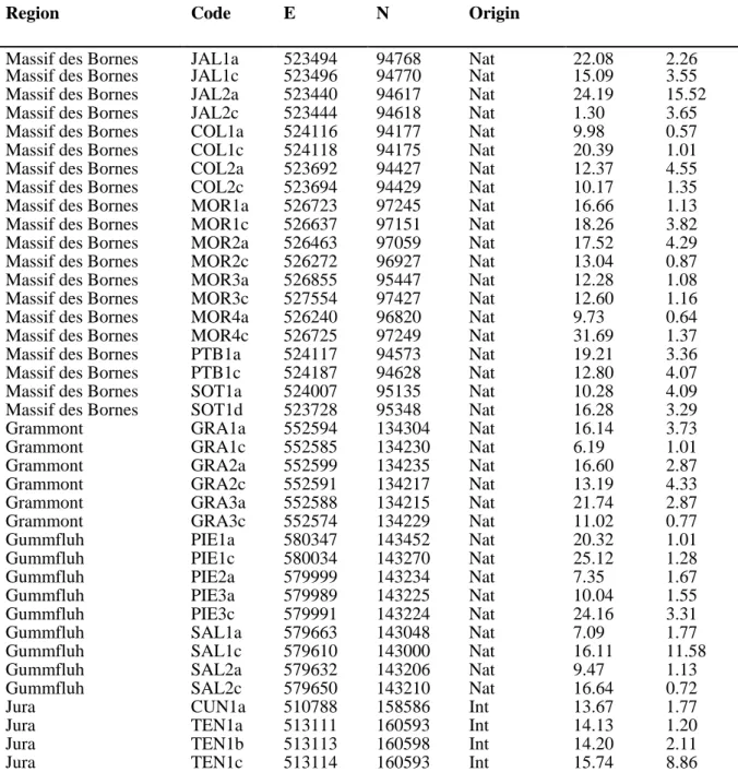
Table S1: Sampling of 136 individuals of the Papaver alpinum complex included here, with name codes as the three first letters of field populations. Coordinates as easternness (E) and northernness (N) in the Swiss Coordinate System. The 112 samples confirmed as native individuals of P. occidentale based on STRUCTURE analyses are indicated as such (Nat), whereas introduced samples (Int) and those genetically pertaining to outgroups P. sendtneri and P. tatricum (Out) are indicated. The mean read depth (DP) and proportion of SNPs with missing data (%NAs) are shown for each sample
Region Code E N Origin
DP %NAs
Massif des Bornes JAL1a 523494 94768 Nat 22.08 2.26 Massif des Bornes JAL1c 523496 94770 Nat 15.09 3.55 Massif des Bornes JAL2a 523440 94617 Nat 24.19 15.52 Massif des Bornes JAL2c 523444 94618 Nat 1.30 3.65 Massif des Bornes COL1a 524116 94177 Nat 9.98 0.57 Massif des Bornes COL1c 524118 94175 Nat 20.39 1.01 Massif des Bornes COL2a 523692 94427 Nat 12.37 4.55 Massif des Bornes COL2c 523694 94429 Nat 10.17 1.35 Massif des Bornes MOR1a 526723 97245 Nat 16.66 1.13 Massif des Bornes MOR1c 526637 97151 Nat 18.26 3.82 Massif des Bornes MOR2a 526463 97059 Nat 17.52 4.29 Massif des Bornes MOR2c 526272 96927 Nat 13.04 0.87 Massif des Bornes MOR3a 526855 95447 Nat 12.28 1.08 Massif des Bornes MOR3c 527554 97427 Nat 12.60 1.16 Massif des Bornes MOR4a 526240 96820 Nat 9.73 0.64 Massif des Bornes MOR4c 526725 97249 Nat 31.69 1.37 Massif des Bornes PTB1a 524117 94573 Nat 19.21 3.36 Massif des Bornes PTB1c 524187 94628 Nat 12.80 4.07 Massif des Bornes SOT1a 524007 95135 Nat 10.28 4.09 Massif des Bornes SOT1d 523728 95348 Nat 16.28 3.29
Grammont GRA1a 552594 134304 Nat 16.14 3.73
Grammont GRA1c 552585 134230 Nat 6.19 1.01
Grammont GRA2a 552599 134235 Nat 16.60 2.87
Grammont GRA2c 552591 134217 Nat 13.19 4.33
Grammont GRA3a 552588 134215 Nat 21.74 2.87
Grammont GRA3c 552574 134229 Nat 11.02 0.77
Gummfluh PIE1a 580347 143452 Nat 20.32 1.01
Gummfluh PIE1c 580034 143270 Nat 25.12 1.28
Gummfluh PIE2a 579999 143234 Nat 7.35 1.67
Gummfluh PIE3a 579989 143225 Nat 10.04 1.55
Gummfluh PIE3c 579991 143224 Nat 24.16 3.31
Gummfluh SAL1a 579663 143048 Nat 7.09 1.77
Gummfluh SAL1c 579610 143000 Nat 16.11 11.58
Gummfluh SAL2a 579632 143206 Nat 9.47 1.13
Gummfluh SAL2c 579650 143210 Nat 16.64 0.72
Jura CUN1a 510788 158586 Int 13.67 1.77
Jura TEN1a 513111 160593 Int 14.13 1.20
Jura TEN1b 513113 160598 Int 14.20 2.11
2
Vanil Noir COM1a 577026 152436 Nat 9.78 5.68
Vanil Noir COM1c 577055 152432 Nat 17.69 12.33
Vanil Noir COM2a 577125 152334 Nat 16.80 1.45
Vanil Noir COM2c 577189 152299 Nat 10.08 4.51
Vanil Noir COM3a 577140 152353 Nat 11.38 1.55
Vanil Noir COM3c 577180 152257 Nat 15.36 3.94
Vanil Noir PAR1a 576800 151454 Nat 15.95 0.71
Vanil Noir PAR1c 576820 151445 Nat 11.27 4.70
Vanil Noir PAR2a 576842 151414 Nat 19.54 5.22
Vanil Noir PAR2c 576830 151427 Nat 10.66 2.50
Vanil Noir PAR3a 576849 151413 Nat 17.27 3.28
Vanil Noir PAR3c 576851 151411 Nat 15.97 2.45
Vanil Noir STJ1a 576436 151924 Nat 13.67 3.77
Vanil Noir STJ1c 576445 151909 Nat 10.28 0.30
Vanil Noir STJ2a 576450 151905 Nat 16.28 4.41
Vanil Noir STJ2c 576440 151928 Nat 13.23 1.99
Vanil Noir STJ3a 576472 151926 Nat 17.56 1.94
Vanil Noir STJ3c 576483 151950 Nat 21.66 4.78
Vanil Noir STJ4a 576554 151770 Nat 10.00 20.9
Vanil Noir STJ4c 576687 151826 Nat 12.47 1.53
Vanil Noir VEC1a 577021 152648 Nat 22.13 0.54
Vanil Noir VEC1c 577004 152665 Nat 13.44 5.68
Vanil Noir VEC2d 576970 152744 Nat 14.13 0.91
Vanil Noir VEC2e 576932 152705 Nat 21.12 4.36
Vanil Noir VEC3a 576877 152665 Nat 18.29 0.81
Vanil Noir VEC3c 576854 152626 Nat 10.63 1.48
Vanil Noir VEC4a 576799 152663 Nat 21.09 1.08
Vanil Noir VEC4c 576783 152658 Nat 23.76 1.86
Dent de Savigny RUT1a 584494 156069 Nat 23.92 3.11 Dent de Savigny RUT1c 584554 156073 Nat 11.15 2.06
Dent de Savigny RUT2a 584606 156028 Nat 9.79 1.50
Dent de Savigny RUT2c 584623 156126 Nat 14.99 3.58 Dent de Savigny RUT3a 584726 156032 Nat 16.70 0.72 Dent de Savigny RUT3c 584807 156035 Nat 12.04 6.34 Dent de Savigny SAV1a 583809 155591 Nat 23.14 0.74 Dent de Savigny SAV1c 583832 155598 Nat 10.45 2.57 Dent de Savigny SAV2a 583920 155659 Nat 29.93 5.68 Dent de Savigny SAV2c 583871 155673 Nat 13.73 3.02
Spillgerten FRO1a 599739 154462 Nat 21.78 2.52
Spillgerten FRO1c 599689 154493 Nat 18.50 0.89
Spillgerten FRO2a 599554 154550 Nat 21.86 0.38
Spillgerten FRO2c 599533 154555 Nat 14.61 1.52
Spillgerten FRO3a 599448 154555 Nat 14.39 1.53
Spillgerten FRO3c 599356 154609 Nat 27.63 1.65
Spillgerten FRO4a 599230 154542 Nat 25.57 0.37
Spillgerten FRO4c 599256 154501 Nat 17.24 0.98
Spillgerten GAN1a 598875 152925 Nat 14.72 98.64
Spillgerten GAN1c 598856 153069 Nat 17.66 3.41
Spillgerten GAN2a 598858 152946 Nat 11.42 2.48
Spillgerten GAN2c 598878 152976 Nat 10.44 1.15
Spillgerten GAN3a 598802 153036 Nat 9.70 1.30
Spillgerten GAN3c 598763 152991 Nat 10.97 1.09
Spillgerten GAN4c 598663 152997 Nat 15.32 2.90
Spillgerten HFR1a 600367 154424 Nat 13.20 4.55
Spillgerten HFR1c 600488 154282 Nat 12.90 1.01
Spillgerten HFR2a 600517 154290 Nat 23.91 0.16
Spillgerten HFR2c 600432 154194 Nat 14.83 0.32
Spillgerten HFR3a 600479 154357 Nat 11.41 0.13
Spillgerten HFR3c 600486 154339 Nat 14.48 0.32
Spillgerten HFR4a 600455 154236 Nat 21.84 0.96
3
Spillgerten HFR5a 600271 154210 Nat 15.59 1.52
Spillgerten HFR5c 600286 154226 Nat 12.56 4.60
Spillgerten HFR6a 600307 154160 Nat 10.85 0.38
Spillgerten HFR6c 600167 154186 Nat 21.21 6.00
Spillgerten HOL1a 599346 154100 Nat 11.30 4.88
Spillgerten HOL1c 599325 154128 Nat 25.74 1.28
Spillgerten HOL2a 599503 154137 Nat 11.07 0.69
Spillgerten HOL2c 599732 154105 Nat 6.50 1.87
Spillgerten VSP1a 599784 153988 Nat 11.97 0.74
Spillgerten VSP1c 599838 153987 Nat 16.13 0.10
Spillgerten VSP2a 599843 153989 Nat 23.82 2.50
Spillgerten VSP2c 599879 153989 Nat 17.56 0.30
Spillgerten VSP3a 599902 153995 Nat 25.50 0.59
Spillgerten VSP3c 600008 153939 Nat 15.66 0.42
Spillgerten VSP4a 600070 153910 Nat 12.65 0.23
Spillgerten VSP4b 600167 153897 Nat 18.46 1.94
Lucerne BLA1a 644462 182601 Out 16.39 0.65
Lucerne BLA1c 644466 182597 Out 14.20 0.96
Lucerne BLA2a 644472 182535 Out 9.40 2.77
Lucerne BLA3a 644440 182711 Out 14.79 0.67
Lucerne BLA3b 644439 182705 Out 13.73 2.55
Lucerne BLA4a 644650 182748 Out 17.41 1.09
Lucerne BLA5a 644674 182775 Out 10.77 1.42
Lucerne BLA5b 644730 182954 Out 24.97 4.26
P. sendtneri PSe1 659990 204424 Out 17.13 na
P. sendtneri PSe2 659995 204419 Out 10.79 na
P. sendtneri PSe3 659987 204414 Out 10.75 na
P. sendtneri PSe4 659970 204403 Out 19.44 na
P. tatricum PTa1_3 NA NA Out 14.88 4.16
P. tatricum PTa2_3 NA NA Out 11.09 0.49
P. tatricum PTa3_3 NA NA Out 14.48 5.39
P. tatricum PTa4_3 NA NA Out 11.10 0.40
P. tatricum PTa1a NA NA Out 17.55 0.93
P. tatricum PTa1b NA NA Out 17.76 1.13
P. tatricum PTa2a NA NA Out 24.44 2.04
4
Table S2: Filtering of raw SNPs to generate dataset, with number of SNPs retained at each step
Filtering step Number
of SNPs
Total raw SNPs 338463
Removal of quality (Q<20), Min depth (<3), Mean depth (<10), Minor
Allele Count (<3), Minor Allele frequency (<0.05) and missing data (>0.5) 45604
Removal of sites with too many NAs (0.2) per population 41350
Filter for allele balance and mapping quality 18251
Removal of loci with extreme high coverage 17676
Decomposition of complex SNPs 21314
Removal of indels, sites with missing data (0.9) and non-biallelic sites 18941
Removal of sites deviating from (global) Hardy-Weinberg (SNPs) 5912
Rad_haplotyper (independent ddRAD loci) 3070
Removal of putatively non-neutral ddRAD loci 2369
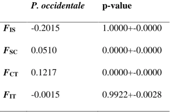
Table S3: Partitioning of genetic structure among the 112 native individuals (I) of Papaver
occidentale nested in field populations (S) and sampling regions (C) from hierarchical
AMOVA on 3070 ddRAD loci P. occidentale p-value
FIS -0.2015 1.0000+-0.0000
FSC 0.0510 0.0000+-0.0000
FCT 0.1217 0.0000+-0.0000
5
Table S4: Pairwise FST between the 19 native populations of P. occidentale. Significant differences are noted in bold
COL JAL MOR PTB SOT GRA PIE SAL COM PAR STJ VEC RUT SAV FRO GAN HFR HOL VSP
COL 0 JAL -0.007 0 MOR 0.0601 0.0794 0 PTB -0.027 -0.024 0.0771 0 SOT -0.042 -0.028 0.0505 -0.061 0 GRA 0.1647 0.173 0.1841 0.1597 0.1579 0 PIE 0.1239 0.1364 0.1625 0.1304 0.1132 0.1983 0 SAL 0.1334 0.14 0.1697 0.1352 0.1192 0.2021 -0.017 0 COM 0.1069 0.1185 0.1462 0.1005 0.0967 0.1686 0.1347 0.1387 0 PAR 0.1588 0.1688 0.1903 0.1618 0.1491 0.2214 0.1753 0.1808 0.0547 0 STJ 0.137 0.1446 0.1652 0.1337 0.1236 0.1935 0.1547 0.1613 0.0313 0.0601 0 VEC 0.1258 0.1341 0.16 0.1138 0.111 0.1772 0.1427 0.1543 0.0033 0.077 0.0488 0 RUT 0.1478 0.1547 0.1729 0.1531 0.1353 0.2106 0.1704 0.1782 0.1458 0.1929 0.1742 0.1532 0 SAV 0.1309 0.1409 0.1643 0.1462 0.132 0.2076 0.1547 0.1754 0.1432 0.1899 0.1654 0.1448 0.0323 0 FRO 0.1256 0.1208 0.1516 0.1164 0.1027 0.1833 0.143 0.1497 0.1364 0.1799 0.162 0.1447 0.1663 0.1593 0 GAN 0.1339 0.1266 0.1543 0.1218 0.1074 0.2013 0.1515 0.1603 0.1548 0.1952 0.1762 0.1592 0.1674 0.1552 0.0536 0 HFR 0.1143 0.1061 0.1362 0.0979 0.0881 0.1611 0.1217 0.1302 0.1214 0.1587 0.1399 0.132 0.1435 0.1333 0.0072 0.0398 0 HOL 0.1291 0.1289 0.1566 0.1179 0.1024 0.1997 0.1681 0.1729 0.1452 0.1978 0.1706 0.1545 0.1788 0.1748 0.0415 0.067 0.029 0 VSP 0.1085 0.1031 0.1343 0.0971 0.0766 0.1644 0.133 0.1397 0.1255 0.1671 0.1423 0.1347 0.1488 0.1437 0.0193 0.0358 0.0071 0.0116 0
6
Figure S1: Barplots presenting the hierarchical genetic clustering of samples of Papaver occidentale among regions using STRUCTURE on different
datasets: all 136 samples (incl. outgroups) vs 112 native samples of P. occidentale at all 3070 ddRAD loci vs 2369 ddRAD loci (i.e. after exclusion of 701 genic loci). On the right, evaluation of optimal number of clusters (K) according to ΔK (‘Evanno’) method and the mean Ln probabilities. All datasets highlight similar genetic structure within P. occidentale.
7
Supplementary Text S1: Species Distribution Modelling (SDM) based on present
occurrence data used to evaluate the potential distribution range of Papaver occidentale at current time and describe putative locations of suitable habitats during the LGM, following Fragnière et al. (2020).
Environmental variables likely playing a role in the distribution of P. occidentale distribution were selected from different available sources at the finest resolution (10 m; table). For SDM based here on presence at 28,209 coordinates across the currently occupied area, the following variable were used SLOPE, NORTHNESS, TEMP, PREC_Sum, PREC_Win, SUNSHINE, IRRAD, HOURS_SUN and SCREES, following Fragnière et al. (2020). The indirect variable ELEVATION was neglected (Guisan et al. 2017) and temperature (TEMP), which is more direct and suitable for predictions across time, was privileged. SCREES explained most of the current distribution of P. occidentale and was removed from models to unmask the effect of other variables. As the original data for temperature at 1 km resolution was highly correlated with ELEVATION (R-squared value = 0.92, p-value < 0.001), TEMP was downscaled at a 10 m resolution based on ELEVATION. Multicollinear variables were removed (R-squared values > 0.6; Menard 2002) with a high variance inflation factor (VIF>5; Guisan et al. 2017).
Table. Environmental variables initially selected for current SDM of P. occidentale.
Abbreviation Variable type Unit Source Native
resolution Resolution used in SDM
SLOPE terrain inclination
Degrees (°) From DEM 2 m Upscaled to 10 m, median value
NORTHNESS Slope aspect on the south-north axis
No unit, a real number between -1 (south) and 1 (north)
From DEM, cosinus of the slope aspect
2 m Upscaled to 10 m, median value
TEMP Mean yearly mean temperature (norm, 1981-2010) degrees °C TnormY8110 (Meteoswiss, 2018) 1000 m Downscaled to 10 m, using DEM to improve resolution (strong negative linear relationship between ELEVATION and TEMP, R-squared value = 0.92, p-value < 0.001 ***. TEMP was thus calculated as a function of ELEVATION, see Online Resource 4)
PREC_Win Mean winter precipitation (norm, 1981-2010)
Milimeters (mm) RnormM8110, mean for December, January and February (Meteoswiss, 2018)
1000 m Downscaled to 10m, using bicubic spline interpolation to get a smooth result SUNSHINE Mean yearly
relative sunshine duration (norm, 1981-2010) Percent (%) SnormY8110 (Meteoswiss, 2018) 1000 m Downscaled to 10m, using bicubic spline interpolation to get a smooth result
IRRAD Total irradiance during one day at the solstice (21 of June)
Wh / m2 /day From DEM with r.sun (Solar irradiance and irradiation model) in GRASS GIS (Neteler and Mitasova, 2013)
10 m 10 m
HOURS_SUN Hours of sun during one day at the solstice (21 of June)
Hours (h) From DEM with r.sun (Solar irradiance and irradiation model) in GRASS GIS 10 m 10 m SCREES Landcover : area with Calcareous screes Presence-absence (1-0)
Area delimited using GEOCOVER and orthophotos with a 100 m buffer. NA, vector data. Rasterized to10 m
8
Model selection, calibration and validation
Pseudo-absence data (or background data) representative of random environmental conditions across the studied area were generated as to equal the number of presences (i.e. 28,209).
Following comparison of general linear and additive models (Fragnière et al. 2020), we here used a General Additive Model (GAM) with logit as link function and included nonlinear smooth functions of environmental variables (k set to 2) in the SDM (Guisan et al. 2002; Hastie et al. 2017). All environmental variables were initially included in the models and their significance estimated to remove some superfluous variables and build to the most parsimonious model based on the Akaike information criterion (AIC) and Bayesian information criterion (BIC; Atkinson 1980; Sakamoto et al. 1986).
As our data were strongly spatially autocorrelated, cross validation techniques such as the 10-fold cross validation (Rodriguez et al. 2009; Lever et al. 2016) and Monte-Carlo cross validation (Shao 1993; Xu and Liang 2001) were unsuitable. We therefore designed a spatial cross validation (Pohjankukka et al. 2017; Roberts et al. 2017) and split the studied area into two blocks along the W-E axis to use data within one block to train the model while data from the second block validated the model, and vice versa. This procedure was repeated along the N-S axis and environmental variables underlying overfitting were accordingly removed. Cross validation was analyzed with a ROC curve (Hanley and McNeil 1982), plotting the true positive rate against false positive rate for each validation dataset next to the full model ROC curve and using the area under the curve (AUC) and mean squared residuals (MSR) to evaluate the model performance.
The validated GAM model predicting P. occidentale habitat suitability across screes of its native distribution included four significant environmental variables (SLOPE, TEMP, NORTHING, PREC_Win; p-value < 0.001) and explained 58.64 % of the total variance. The mean AUC of the validation datasets during the spatial cross validation was 0.9 and a best threshold from the ROC curve estimated at 0.55.
References
Atkinson, A. C. (1980) A note on the generalized information criterion for choice of a model. Biometrika 67:413-418.
Fragnière Y, Pittet L, Clément B, Bétrisey S, Gerber E, Ronikier M, Parisod C, Kozlowski G (2020) Climate change and alpine screes: no future for glacial relict Papaver occidentale (Papaveraceae) in Western Prealps. Submitted.
Guisan A, Edwards Jr TC, Hastie T (2002) Generalized linear and generalized additive models in studies of species distributions: setting the scene. Ecol Model 157:89-100.
Guisan A, Thuiller W, Zimmermann NE (2017) Habitat suitability and distribution models: with applications in R. Cambridge University Press.
9
Hanley JA, McNeil BJ (1982) The meaning and use of the area under a receiver operating characteristic (ROC) curve. Radiology 143:29-36.
Hastie TJ (2017) Generalized additive models. In Statistical models in S (pp. 249-307). Routledge.
Lever J, Krzywinski M, Altman N (2016) Points of significance: model selection and overfitting. Nat Methods 13:703–704.
Menard S (2002). Applied logistic regression analysis (Vol. 106). Sage.
Pohjankukka J, Pahikkala T, Nevalainen P, Heikkonen J (2017) Estimating the prediction performance of spatial models via spatial k-fold cross validation. Int J Geogr Inf Sci 31:2001-2019.
Roberts DR, Bahn V, Ciuti S, Boyce MS, Elith J, Guillera‐Arroita G, Hauenstein S, Lahoz-Monfort JJ, Schröder B, Thuiller W, Warton DI, Wintle BA, Hartig F, Dormann CF (2017) Cross‐validation strategies for data with temporal, spatial, hierarchical, or phylogenetic structure. Ecography 40:913-929.
Rodriguez JD, Perez A, Lozano JA (2009) Sensitivity analysis of k-fold cross validation in prediction error estimation. IEEE Transactions on Pattern Analysis and Machine Intelligence 32:569-575.
Sakamoto Y, Ishiguro M, Kitagawa G (1986) Akaike information criterion statistics. Dordrecht, The Netherlands: D. Reidel 81.
Shao J (1993) Linear model selection by cross-validation. J Am Stat Assoc 88:486-494. Xu QS, Liang YZ (2001) Monte Carlo cross validation. Chemomet Intell Lab Syst 56:1-11.