HAL Id: hal-01965451
https://hal-amu.archives-ouvertes.fr/hal-01965451
Submitted on 26 Dec 2018
HAL is a multi-disciplinary open access
archive for the deposit and dissemination of
sci-entific research documents, whether they are
pub-lished or not. The documents may come from
teaching and research institutions in France or
abroad, or from public or private research centers.
L’archive ouverte pluridisciplinaire HAL, est
destinée au dépôt et à la diffusion de documents
scientifiques de niveau recherche, publiés ou non,
émanant des établissements d’enseignement et de
recherche français ou étrangers, des laboratoires
publics ou privés.
Distributed under a Creative Commons Attribution| 4.0 International License
Nonadiabatic Excited-State Dynamics with Machine
Learning
Pavlo Dral, Mario Barbatti, Walter Thiel
To cite this version:
Pavlo Dral, Mario Barbatti, Walter Thiel. Nonadiabatic Excited-State Dynamics with Machine
Learn-ing. Journal of Physical Chemistry Letters, American Chemical Society, 2018, 9 (19), pp.5660-5663.
�hal-01965451�
Nonadiabatic Excited-State Dynamics with Machine Learning
Pavlo O. Dral,
*,†Mario Barbatti,
*,‡and Walter Thiel
*,††Max-Planck-Institut für Kohlenforschung, Kaiser-Wilhelm-Platz 1, 45470 Mülheim an der Ruhr, Germany ‡Aix Marseille Univ, CNRS, ICR, Marseille, France
Supporting Information Placeholder
ABSTRACT: We show that machine learning (ML) can be used to accurately reproduce nonadiabatic excited-state dynamics with decoherence-corrected fewest switches surface hopping in a one-dimensional model system. We propose to use ML to significantly reduce the simulation time of realistic, high-dimensional systems with good reproduction of observables obtained from reference simulations. Our approach is based on creating approximate ML potentials for each adiabatic state using a small number of training points. We investigate the feasibility of this approach by using adiabatic spin-boson Hamiltonian models of various dimensions as reference methods.
TOC GRAPHICS
Excited-state dynamics simulations of molecules and molecular assemblies are as important as challenging. Some of the primary processes in nature (photosynthesis, light detection), medicine (phototherapy, DNA damage), and technology (photovoltaics, photonics) have at least one photoinduced reaction step occurring in the excited state.1-3 The main difficulties in modeling these
processes arise from the intricacies of excited-state electronic structure and from the intrinsic nonadiabaticity caused by the coupling between nuclear and electronic degrees of freedom driving the time evolution.
Significant advances in the simulation of nonadiabatic dynam-ics in excited states have been achieved in recent years.4 The development of on-the-fly nonadiabatic mixed quantum-classical (NA-MQC) strategies, in particular, has boosted the research field in the last decade allowing full-dimensional simulations of sys-tems with tens of atoms for several picoseconds. In these methods nonadiabatic phenomena are introduced into a classical ensemble
of trajectories through averaging, spawning, or hopping of quan-tum electronic information. At the same time, they rely on a local approximation allowing for the computation of electronic proper-ties only at the classical nuclear coordinates.
The on-the-fly strategy is a fundamental advantage, as it avoids the costly calculation of multi-dimensional potential energy sur-faces (PESs)—a task that is the main bottleneck in full quantum approaches. However, the on-the-fly propagation of the dynamics is computationally demanding, because expensive quantum me-chanical (QM) quantities—energies, forces, and couplings be-tween the electronic states—must be computed at each time step in the numerical integration of the equations of motion. Conse-quently, an on-the-fly NA-MQC simulation of a medium-sized molecule for several picoseconds may require hundreds of thou-sands of CPU hours when using first-principles QM methods.
The emergence of machine learning (ML) algorithms has the potential to change this scenario, ideally leading to situations where ML inexpensively predicts excited-state energies, forces, and couplings for on-the-fly NA-MQC dynamics. Encouragingly, ML has already been successfully applied in many atomistic simulations, for example to represent PESs, to perform molecular dynamics in the ground state and to predict excited-state proper-ties.5-22 However, the application of ML to on-the-fly NA-MQC dynamics poses unique challenges. Among the most crucial prob-lems is the higher complexity of the excited-state electronic struc-ture, often leading to a high density of coupled states, with a strongly anharmonic dependence on nuclear coordinates. Moreo-ver, in many cases, the nonadiabatic processes happen on time scales shorter than those of thermal equilibration, requiring prop-agation of microcanonical rather than canonical ensembles, which are associated with much stricter conservation requirements.
Only few recent studies have attempted to use ML for such purposes. In a pilot study of ML-enhanced NA-MQC dynamics, ML was used only for the representation of the relevant PESs; however, the generation of training points was rather tedious and time consuming, while the number of QM calculations performed during the training of the ML models and during the dynamics was close to the number of QM calculations typically required for a corresponding on-the-fly QM simulation.6 In another study, the accuracy of direct quantum wavepacket dynamics with ML PESs was shown to deteriorate quickly with increasing number of di-mensions so that it became problematic to achieve good accuracy even for as few dimensions as six.17
The main aim of our work is to outline how ML can be used to achieve a significant reduction of the number of required QM calculations in practical on-the-fly NA-MQC simulations of high-dimensional systems. For this purpose we use the popular decoherence-corrected fewest switches surface hopping
(DC-FSSH, see the Supporting Information, SI) approach in on-the-fly NA-MQC dynamics and an ML approach based on kernel ridge regression (KRR, see SI for details). To avoid any bias associated with the choice of a specific QM method and a target molecule, we decided to use the two-state spin-boson Hamiltonian in the adiabatic representation (A-SBH, see SI), which is easily adjusta-ble in terms of the number of degrees of freedom and couplings. This choice of an analytical Hamiltonian allows for an extensive and general assessment of ML capabilities because we can com-pute many more trajectories and time steps than we would be able to do with any on-the-fly electronic structure method. Note, how-ever, that the use of A-SBH does not lead to any loss of generali-ty, as every element of an atomistic two-state simulation is present in this model, and the generalization to more states is straightfor-ward. As discussed below, because of the strong coupling between different A-SBH dimensions, ML-based NA-MQC dy-namics may in some aspects even be more challenging for A-SBH than for an atomistic model.
We start by demonstrating for the one-dimensional (1-D) A-SBH model that it is possible, in principle, to create a complete ML model, which can accurately reproduce the reference A-SBH trajectory with all hopping events (Figure 1). This is achieved when using at least Ntr = 128 points in the training set (see SI for
further details).
Figure 1. Comparison of A-SBH and complete ML surface
hop-ping trajectories for the 1-D model: The simulations started from the same initial conditions and were run with the same random seed.
For high-dimensional systems, it is generally not feasible to build such complete ML models. First, generating a sufficient amount of accurate QM reference data quickly becomes too costly due to the curse of dimensionality. For a realistic 33-D model it would be necessary to calculate reference values for 12833 =
3.45∙1069
grid points to ensure sampling with the same density as for our complete 1-D ML model (Figure 1).23 This is obviously impossible. Second, processing large amounts of reference data is also very challenging, both in terms of memory requirements and training time. Third, if the number of training points for ML becomes too large, it may be more reasonable to run pure QM dynamics. Thus, for ML to significantly speed up nonadiabatic dynamics simulations, the training set has to be as small as possi-ble and to be generated as quickly as possipossi-ble.
In practical terms, our first aim is to keep the number of points in the training set preferably at most 10,000 points. For compari-son, ground-state ML potentials have been trained on many fewer
molecular geometries and used successfully for various purposes such as molecular dynamics, calculation of vibrational spectra, and geometry optimization.7, 14-15 From our experience with on-the-fly NA-MQC dynamics based on ab initio and semiempirical methods, we know that these simulations are typically run with about 100 trajectories with a time step of 0.5 fs for 1 ps, i.e. they require 200,000 QM calculations. Therefore, 10,000 points repre-sents merely 5% of a typical on-the-fly NA-MQC project. Moreo-ver, the gains are potentially much larger. Although 100 trajecto-ries are enough to reveal all main reaction pathways, their path-way yields are delivered with rather low precision. However, after training the machine, it can be used to run thousands of trajecto-ries, producing highly precise results, which would simply be unaffordable with conventional QM approaches.
Proposed approaches for generating training sets are often itera-tive and rather time consuming.15 Our second aim is to avoid such
handicaps and keep the construction of the training set as simple and inexpensive as possible.
Based on these considerations, we target a relatively sparse grid of training points, sampled with a low discrepancy algorithm.7, 24 Inevitably, this will lead to some loss of accuracy. However, it is known that ML trained on points sampled along vibrational modes can describe larger molecules and also give rather accurate PESs.18 Furthermore, very accurate ML PES can be obtained for small molecules.7
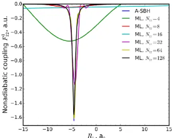
The most serious additional challenge in the case of DC-FSSH dynamics is that the nonadiabatic couplings feature sharp, narrow spikes around certain geometries (Figure 2). This necessitates very small time steps or special treatments even in the pure QM DC-FSSH dynamics.25 Sparse sampling of ML training points will in most cases miss these spikes (Figure 2), and consequently no or too few hops will happen during ML dynamics.
Figure 2. Comparison of nonadiabatic couplings calculated for
the A-SBH and ML models trained on an increasing number of points for the 1-D model.
Indeed, we find no hops at all in 2 ps trajectory produced with an ML model of the 1-D system trained on only 16 points (Figure S1), compared with 4 hops when we calculate nonadiabatic cou-plings with A-SBH throughout the trajectory (Figure S2). In previous work on ML for FSSH,6 the Zhu−Nakamura approach26 was used to avoid the calculation of nonadiabatic couplings alto-gether. Here we solve this problem by performing QM (in this work A-SBH) calculations of nonadiabatic couplings instead of estimating them with ML when the band gap estimated with ML is small. A similar approach was tested for the Zhu−Nakamura
dynamics for a different reason (to avoid errors of the ML poten-tial in the vicinity of the conical intersections).6 In the case of our
1-D ML model trained on 16 points, 5 hops occur if we switch on A-SBH calculations for 𝑉2est− 𝑉1est < 0.03 Hartree (Figure S3).
We use this cutoff in the following. Problems with sparse sam-pling concerning total energy conservation are discussed in the SI. Next, we compare the performance of ML dynamics with A-SBH simulations for a realistic 33-D system. This system is rather challenging for ML, as exemplified by the fact that during a 50 ps A-SBH trajectory the smallest Euclidian distance between a point at a given time step to any point visited during first 80% of previ-ous time steps remained very large and did not decrease over time. This means that the same region in the high-dimensional space was not visited again during the 50 ps nonadiabatic dynam-ics. Consequently, all our attempts to use on-the-fly or adaptive learning strategies commonly employed in ground-state ML dynamics for atomistic systems16, 22 failed for our 33-D A-SBH system. This may be attributed to the strong coupling between different of A-SBH dimensions, while in atomistic simulations it is often possible to partition the system into smaller, sufficiently independent sub-structures.13, 15, 18, 22
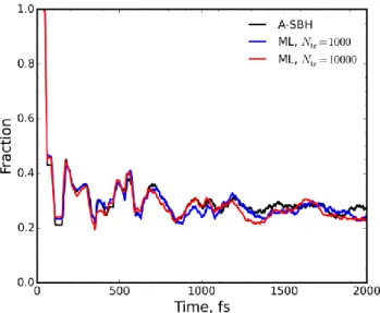
In order to collect enough data for statistical analysis, we ran 1,000 trajectories with A-SBH and various ML models, each starting on the S1 surface. We trained two different ML models,
on 1,000 and on 10,000 points. The evolution of the S1 state
popu-lation during 2 ps dynamics is reproduced very well by both ML models (Figure 3) despite the relatively small training sets gener-ated in a simple, non-iterative manner. The excited-state lifetime is estimated (see SI) to be 114 ± 1, 100 ± 1, and 105 ± 1 fs with A-SBH, ML trained on 1,000 points, and ML trained on 10,000 points, respectively. The ML lifetimes are thus in reasonable agreement with the A-SBH lifetime. An additional comparative analysis is provided in the SI.
Figure 3. Evolution of the fraction of trajectories on state S1 along
A-SBH (black) and ML (blue, red) surface hopping trajectories for the 33-D model averaged for 1,000 trajectories. The ML mod-els were trained on 1,000 and 10,000 points, respectively.
In our ML dynamics, A-SBH calculations during DC-FSSH dynamics were invoked only in 13–16% of time steps for 𝑉2est− 𝑉1est < 0.03 Hartree. Such QM calculations should be
avoided in the future altogether by using local diabatization, which eliminates the problem with narrow couplings.27 In this case, the cost of ML nonadiabatic dynamics will be essentially determined by the cost of training set generation.
In summary, we show that ML can be used to simulate accu-rate, multidimensional nonadiabatic dynamics with significant cost reduction. We suggest using fairly sparse small training sets sampled from the high-dimensional space to build approximate ML potentials for each adiabatic surface. We show that dynamics runs with these ML potentials well reproduce the time evolution of the adiabatic state population and the excited-state lifetime obtained from the dynamics with the reference method.
AUTHOR INFORMATION
Corresponding Authors
*E-mail: dral@kofo.mpg.de. Website: dr-dral.com
*E-mail: mario.barbatti@univ-amu.fr. Website: www.barbatti.org *E-mail: thiel@kofo.mpg.de
Notes
The authors declare no competing financial interests.
ACKNOWLEDGMENT
MB thanks for support from the Excellence Initiative of Aix-Marseille University (A*MIDEX) and the project Equip@Meso (ANR-10-EQPX-29-01), both funded by the French Government “Investissements d’Avenir” program, and for funding from the WSPLIT project (ANR-17-CE05-0005-01). WT acknowledges support from an ERC Advanced Grant (OMSQC).
ASSOCIATED CONTENT
Supporting Information
The Supporting Information is available free of charge on the ACS Publications website.
Supporting Information Available: Description of methods and
additional technical details on nonadiabatic dynamics (PDF)
REFERENCES
(1) Gozem, S.; Luk, H. L.; Schapiro, I.; Olivucci, M. Theory and Simulation of the Ultrafast Double-Bond Isomerization of Biological Chromophores. Chem. Rev. 2017, 117, 13502–13565.
(2) Akimov, A. V.; Prezhdo, O. V. Large-Scale Computations in Chemistry: A Bird's Eye View of a Vibrant Field. Chem. Rev. 2015, 115, 5797–5890.
(3) Brunk, E.; Rothlisberger, U. Mixed Quantum Mechani-cal/Molecular Mechanical Molecular Dynamics Simulations of Biological Systems in Ground and Electronically Excited States. Chem. Rev. 2015,
115, 6217–6263.
(4) Crespo-Otero, R.; Barbatti, M. Recent Advances and Perspec-tives on Nonadiabatic Mixed Quantum-Classical Dynamics. Chem. Rev.
2018, 118, 7026–7068.
(5) Brockherde, F.; Vogt, L.; Li, L.; Tuckerman, M. E.; Burke, K.; Müller, K.-R. Bypassing the Kohn-Sham Equations with Machine Learn-ing. Nat. Commun. 2017, 8, 872.
(6) Hu, D.; Xie, Y.; Li, X.; Li, L.; Lan, Z. Inclusion of Machine Learning Kernel Ridge Regression Potential Energy Surfaces in On-the-Fly Nonadiabatic Molecular Dynamics Simulation. J. Phys. Chem. Lett.
2018, 9, 2725–2732.
(7) Dral, P. O.; Owens, A.; Yurchenko, S. N.; Thiel, W. Structure-Based Sampling and Self-Correcting Machine Learning for Accurate Calculations of Potential Energy Surfaces and Vibrational Levels. J.
Chem. Phys. 2017, 146, 244108.
(8) Chmiela, S.; Tkatchenko, A.; Sauceda, H. E.; Poltavsky, I.; Schütt, K. T.; Müller, K.-R. Machine Learning of Accurate Energy-Conserving Molecular Force Fields. Sci. Adv. 2017, 3, e1603015.
(9) Hansen, K.; Montavon, G.; Biegler, F.; Fazli, S.; Rupp, M.; Scheffler, M.; von Lilienfeld, O. A.; Tkatchenko, A.; Müller, K.-R. As-sessment and Validation of Machine Learning Methods for Predicting
Molecular Atomization Energies. J. Chem. Theory Comput. 2013, 9, 3404–3419.
(10) Rupp, M. Machine Learning for Quantum Mechanics in a Nut-shell. Int. J. Quantum Chem. 2015, 115, 1058-1073.
(11) Ramakrishnan, R.; Hartmann, M.; Tapavicza, E.; von Lilien-feld, O. A. Electronic Spectra from TDDFT and Machine Learning in Chemical Space. J. Chem. Phys. 2015, 143, 084111.
(12) Unke, O. T.; Meuwly, M. Toolkit for the Construction of Re-producing Kernel-Based Representations of Data: Application to Multidi-mensional Potential Energy Surfaces. J. Chem. Inf. Model. 2017, 57, 1923–1931.
(13) Bartók, A. P.; Csányi, G. Gaussian Approximation Potentials: A Brief Tutorial Introduction. Int. J. Quantum Chem. 2015, 115, 1051– 1057.
(14) Denzel, A.; Kästner, J. Gaussian Process Regression for Ge-ometry Optimization. J. Chem. Phys. 2018, 148, 094114.
(15) Gastegger, M.; Behler, J.; Marquetand, P. Machine Learning Molecular Dynamics for the Simulation of Infrared Spectra. Chem. Sci.
2017, 8, 6924–6935.
(16) Li, Z.; Kermode, J. R.; De Vita, A. Molecular Dynamics with On-the-Fly Machine Learning of Quantum-Mechanical Forces. Phys. Rev.
Lett. 2015, 114, 096405.
(17) Richings, G. W.; Habershon, S. Direct Quantum Dynamics Us-ing Grid-Based Wave Function Propagation and Machine-Learned Poten-tial Energy Surfaces. J. Chem. Theory Comput. 2017, 13, 4012–4024.
(18) Smith, J. S.; Isayev, O.; Roitberg, A. E. ANI-1: An Extensible Neural Network Potential with DFT Accuracy at Force Field Computa-tional Cost. Chem. Sci. 2017, 8, 3192–3203.
(19) Hase, F.; Kreisbeck, C.; Aspuru-Guzik, A. Machine Learning for Quantum Dynamics: Deep Learning of Excitation Energy Transfer Properties. Chem. Sci. 2017, 8, 8419–8426.
(20) Zhang, L.; Han, J.; Wang, H.; Car, R.; E, W. Deep Potential Molecular Dynamics: A Scalable Model with the Accuracy of Quantum Mechanics. Phys. Rev. Lett. 2018, 120, 143001.
(21) Imbalzano, G.; Anelli, A.; Giofré, D.; Klees, S.; Behler, J.; Ceriotti, M. Automatic Selection of Atomic Fingerprints and Reference Configurations for Machine-Learning Potentials. J. Chem. Phys. 2018,
148, 241730.
(22) Botu, V.; Ramprasad, R. Learning Scheme to Predict Atomic Forces and Accelerate Materials Simulations. Phys. Rev. B 2015, 92, 094306.
(23) Hastie, T.; Tibshirani, R.; Friedman, J. The Elements of
Statis-tical Learning: Data Mining, Inference, and Prediction. 2nd ed.;
Springer-Verlag: 2009.
(24) Sobol, I. M.; Asotsky, D.; Kreinin, A.; Kucherenko, S. Con-struction and Comparison of High-Dimensional Sobol' Generators.
Wil-mott 2011, 2011, 64-79.
(25) Wang, L.; Prezhdo, O. V. A Simple Solution to the Trivial Crossing Problem in Surface Hopping. J. Phys. Chem. Lett. 2014, 5, 713– 719.
(26) Zhu, C.; Nakamura, H. The Two‐State Linear Curve Crossing Problems Revisited. III. Analytical Approximations for Stokes Constant and Scattering Matrix: Nonadiabatic Tunneling Case. J. Chem. Phys.
1993, 98, 6208–6222.
(27) Plasser, F.; Granucci, G.; Pittner, J.; Barbatti, M.; Persico, M.; Lischka, H. Surface Hopping Dynamics Using a Locally Diabatic Formal-ism: Charge Transfer in the Ethylene Dimer Cation and Excited State Dynamics in the 2-Pyridone Dimer. J. Chem. Phys. 2012, 137, 22A514.