The crane split and sequencing problem with clearance and yard congestion constraints in container terminal ports

(1)

The Crane Split and Sequencing Problem with Clearance and Yard Congestion Constraints

in Container Terminal Ports by

Shawn Choo

B. Eng (Electrical Engineering) National University of Singapore, 2005

Submitted to the School of Engineering

in Partial Fulfillment of the Requirements for the Degree of

Master of Science in Computation for Design and Optimization

at the

Massachusetts Institute of Technology

September 2006

The author hereby grants to MIT permission to reproduce and to

distribute publicly paper and electronic copies of this thesis document in whole or in part in any medium now known or hereafter created.

Signature of author... .. Computation for Design and Optimization Program

August 11, 2006

Certified by...

David Simchi-Levi Professor of Civil and Environ ntal Engineering

rI

)

sis Supervisor

Accepted by... ... aime ... aim Peraire Professor of Aeronautics and Astronautics ROME_ _ Co-director, Computation for Design and Optimization Program

MASSACHUSETTS INSTITUfE' OF TECHNOLOGY

(2)

(3)

-THE CRANE SPLIT AND SEQUENCING PROBLEM WITH CLEARANCE AND YARD CONGESTION CONSTRAINTS

IN CONTAINER TERMINAL PORTS by

SHAWN CHOO

Submitted to the School of Engineering

on August 11, 2006 in Partial Fulfillment of the Requirements for the Degree of Master of Science in Computation for Design and Optimization

Abstract

One of the steps in stowage planning is crane split and sequencing, which determines the order of container discharging and loading jobs quay cranes (QCs) perform so that the completion time (or makespan) of ship operation is minimized. The vessel's load profile, number of bays and number of allocated QCs are known to port-planners hours before its arrival, and these are input parameters to the problem. The problem is modeled as a large-scale linear IP where the planning horizon is discretized into time intervals and at most one QC can be assigned to a bay at any period. We introduce clearance constraints, which prevent adjacent QCs from being positioned too close to one another, and yard congestion constraints, which prevent yard storage locations from being overly accessed at any time. This makes the model relevant in an industrial setting. We examine the case only a single ship arrives at port, and the case where multiple ships berth at different times in the planning horizon. The berth time of each ship and number of ships arriving is known. The problem is difficult to solve without any special technique applied.

For the single-ship problem, a heuristic approach, which produces high-quality solutions, is developed. A branch-and-price method re-formulates the problem into a set-covering form with huge number of variables; standard variable branching provides optimal solutions very efficiently. For the multiple-ship problem, a solution strategy is developed combining Lagrangian relaxation, branch-and-price and heuristics. After relaxing the yard congestion constraints, the problem decomposes into smaller sub-problems, each involving one ship; the sub-problems are then re-formulated into a column generation form and solved using branch-and-price to obtain Lagrangian solutions and lower-bound values. Lagrangian multipliers are iteratively updated using the sub-gradient method. A primal heuristic detects and eliminates infeasibilities in the Lagrangian solutions which then become an upper bound to the optimal objective. Once the duality gap is sufficiently reduced, the sub-gradient routine is terminated. The availability of efficient commercial modeling software such as OPL Studio and CPLEX allows for larger instances of the problem to be tackled than previously possible.

Thesis Supervisor: David Simchi-Levi,

(4)

(5)

Acknowledgements

Where is the wise man? Where is the scholar?

Where is the philosopher of this age?

Has not God made foolish the wisdom of the world?

-- 1 Corinthians 1:20 (NIV)

I could never fathom myself one day graduating from a university as prestigious and well-regarded as MIT. I claim no credit for myself. Instead, I am fortunate to have the

support and guidance of the following people, to whom I am ebulliently

grateful--Professor David Simchi-Levi, my advisor, for his guidance, direction, patience and understanding, and whose forthcoming words of encouragement kept me plodding on;

Dr Diego Klabj an, University of Illinois at Urbana-Champaign, for the many hours afforded sharing his academic knowledge and practical experience;

Liang Ping Ku and Hein Thuan Loy, PSA Corporation Operations Planning Department, for providing an excellent research topic and insight into real-life industry practices;

Laura Rose and Jocelyn Sales, course administrators, who were most committed to ensuring that our student experience in MIT was smooth and problem-free;

Singapore-MIT Alliance and the Singaporean government, for sponsoring the SMA Graduate Fellowship;

Yimin, my wife and best friend, for your love so unconditionally given in the last 9 years I've known you, and whom I consider the greatest blessing in my life;

And finally, my parents, Lye Heng and Susan Choo, sister, Sabrina, and brother, Samuel, who have given me everything.

(6)

(7)

List of Figures

Figures

1-1 The two operational interfaces in a container terminal system... 12

1-2 A RTG yard crane placing a container on a truck for transport to the quayside... 12

1-3 Horizontal and vertical cross-section of a typical container vessel... 14

1-4 Drawing of quay cranes serving a vessel, with a clearance separating each adjacent cran es... . 15

2-1 Example of an initial feasible column pool for a ship with parameters H = 6, C = 2 an d r = 1 ... . . ... . . 3 3 2-2 Solutions from the exact method applied to problem instances SS1-1 and SS2-3.. 41

2-3 Solutions from the heuristic approach applied to problem instances SS 1-4 and S S 5-1... . . ... . ... 4 2 2-4 Solutions from the branch-and-price approach applied to problem instances S S4-2 and S S 5-1... 42

2-5 Solutions from the heuristic approach applied to problem instances SSP1, SSP2, S S P 3 ... . . 4 3 2-6 Solutions from the branch-and-price approach applied to problem instances SSP 1, S S P 2 ,S S P 3 ... .. 4 3 2-7 Computational time for various values of H, fix T= 125, C = 2, r = 2... 44

2-8 Computational time for various values of T, fix H = 20, C = 2, r = 2... 44

2-9 Computational time for various values of C, fix T = 125, H= 25, r = 2... 44

3-1 Overall procedure of the Lagrangian Relaxation framework... 55

3-2 Overall flow of the branch-and-price algorithm for solving Lagrangian sub-problem s... . . 59

3-3 Example of a column for t=2 and right-hand vector of the master problem in set-partitioning form for H=3, L=2, C=3, r=0... 60

3-4 Illustration of the breakdown of costs by column in an optimal integer solution of M SM P ... . . . .. . . .. . . .. . . .. . . .. . . 63

3-5 Upper and lower bound values vs. sub-gradient iterations for the case of S=2, H1=10, H2= 10, C1=2, C2=2, T1=32, T2=44, wz=1... 80

3-6 Matlab output of problem instance MSD4 using Lagrangian framework... 82

Tables 1 Top 5 container terminals globally and their throughput (in millions), 200 1-2 0 0 3 ... ... .. 16

2-1 Description of the first data set of test problems... 39

2-2 Description of the second data set of practical test problems... 40

2-3 Output and computational performance of the exact model and proposed solution approaches on the first data set... 40

2-4 Output and computational performance of the various methods on second data set... ... . . 4 2 3-1 Description of the data set of test problems for the multiple-ship model... 81

(10)

3-2 Exact solution, LP and Lagrangian cost output and computational performance of the m ultiple-ship data set... 84 3-3 Comparison of computational performance of 'hard' problem instances when

(11)

Chapter

1 Introduction

1.1 Overview of Container Terminal Operations

Today, over 60% of the world's deep-sea cargo is transported in containers onboard ocean-going vessels, and some routes between economically strong and stable countries are containerized up to 100% [1]. The global growth rate for container port throughput in 2002 was reported to be 9.2%, with port traffic reaching a total of 266.3 million TEUs (twenty-foot equivalent units) [2]. Due to this increasing global demand for containerized marine shipping, container terminals have become important components in global

logistics and transportation networks.

A container terminal serves as an interface between land and sea transportation. Its main functions are to receive outbound (export) containers from shippers for loading onto vessels, and to discharge (unload) inbound (import) containers from vessels for picking up by consignees [3]. These terminals also have storage yards for the temporary storage of containers. Container terminals are considered essential infrastructure because they are highly capital-intensive, and specialized equipment are needed to handle and transport containers within the port system; for example, a quay crane can cost upwards of US$10 million.

(12)

Quayside Landside

Stack with RMG

Quay Crane Vehicles _Vehicles

Trucks, Train Vessel

Figure 1-1. The two operational interfaces of a container terminal system

Container terminals can generally be described as having 2 main operational interfaces, quayside and landside. Quayside activities deal with the loading and unloading of ships, while landside involves loading and unloading of containers on or off

external trucks, trains or yard storage locations. Some of the equipment and resources put to use in both interfaces are shown in Figure 1-1. The transportation of containers between the yard storage locations and the quayside is done primarily by trucks

(sometimes known as prime movers) or automated guided vehicles.

The container terminal also has a storage yard which is usually divided into rectangular regions, known as container blocks. Each container block has about six rows for storing containers in stacks, with an additional lane for truck passing. A row may

(13)

have up to 20 stacks placed end-to-end, each of which can be up to 6 levels high. These blocks are served by yard cranes of which there are 3 types, either rail mounted gantry cranes (RMG), rubber tired gantry cranes (RTG) or more recently, overhead bridge cranes (OHBG). Each type of yard crane confers different advantages to port operators; for example, the RTG cranes can be moved from block to block while the RMG and OHBG cranes are fixed, and the use of OHBG cranes allow for increased stack heights. Yard cranes remove and place containers from the stacks directly onto trucks which park in the passing lane while the transfer occurs. Traffic congestion caused by high rates of loading and unloading containers from a particular block is a concern explored in the chapter 3.

Upon a vessel's arrival at the terminal, a container vessel is assigned to a berth for the loading and discharging of containers. Discharged containers are placed onto trucks by quay cranes for transportation to pre-determined storage locations in the yard, awaiting pickup from the local consignee or trans-shipment onto another vessel. Yard cranes lift containers from the trucks onto their assigned stacks; the trucks are then recycled back into usage for other jobs. Similarly for vessel loading, external customers bring their outbound containers into the port using their own trucks and are instructed to which yard storage location their containers have been assigned. Yard cranes remove the container from the customer's truck onto the stack for storage. When the designated vessel arrives, the yard cranes place the export containers onto trucks for transportation to the vessel area, where they are loaded onto the ship by quay cranes.

The operations of a major Asian container terminal are broadly described in [4,5],

while the interested reader is directed to [6] for a general overview of various attributes of container terminal operations. This thesis focuses on quayside operations; relevant terminologies and resources are elaborated upon in the next few sub-sections.

(14)

Containers are steel boxes of dimensions 20 x 8 x 9.5 or 40 x 8 x 9.5 feet. The unit of measurement for the throughput of 20-ft containers is commonly known as a TEU (twenty foot equivalent unit). Each 40-ft container is counted as 2 TEUs.

The advantage of containerized cargo is that they can be loaded and discharged with fewer crane moves and in a shorter time compared to bulk shipment cargo. Because of the uniformity in sizing, the time needed to handle a container is approximately constant if the equipment used and all other factors are equal. Furthermore, the use of standard-sized cargo streamlines the scheduling and controlling of the flow of goods. Other advantages include the protection of cargo against weather and accidental damage. Also, cargo contents do not have to be unpacked and repacked at each point in transfer resulting in a more rapid handling of freight.

1.1.2 Vessels Structure and Ship bays

A vessel is divided along its length into segments known as bays. Within each bay, the vessel is split vertically into 2 parts, the deck and the hatch, separated by a hatch cover. A drawing of the structure of a generic vessel is shown in Figure 1-3. Each bay can accommodate several rows of containers across and several tiers deep. It is not uncommon for some larger-capacity vessels today to have up to 25 bays, carrying a total of over 9,000 TEUs. These deep-sea vessels have on deck, containers stowed 8 tiers high and 17 rows wide, and in the hatch, 9 deep and 15 rows wide.

A bay is 20-ft wide and can be loaded by 40-ft containers or 20-ft containers. 20-ft container bays are usually odd-numbered, while 40-ft container bays, which occupy twice the length of the former, are evenly-numbered. For example, bays numbered 5 and 7

Row

tauu

I niu*

*n5w mu m

'

000

~~flflflfll R 0000

)Tier

- - - Asingle bay ₀₀ F. H* s of ta 0i 04 0 0

(15)

maybe joined together for loading of 40-ft containers and renamed bay 6.

1.1.3 Quay Cranes

Quay cranes (QC) are, in general, relatively immobile compared to yard cranes which can serve a large region in the storage area. QCs have 4 legs each and the space in between each of the 2 rows of legs is divided into traffic lanes for trucks to pass under. A trolley moves along the arm of the crane and is equipped with a spreader, which is used to pick up containers from the vessel or truck.

QC1

Figure 1-4. Drawing of quay cranes serving a vessel, with a clearance separating each adjacent crane

The width of a typical QC is 25.8 meters, and its practical performance is in the range of 22-30 boxes/hour. It is usual practice for up to 5 QCs to be allocated to large vessels, and up to 2,000 TEUs to be loaded and discharged per vessel in large ports. Port operators usually enforce a work rule that a certain distance, known as clearance, between two adjacent working QCs must be observed for safety reasons and unobstructed operation. QCs run on tracks parallel to the berth line; this horizontal movement is known

as gantrying. Gantrying into position is usually completed in under a minute, lesser time

than needed to handle a container.

Trucks queue up under their allocated QCs, and wait for their container to be picked up. For most efficient operation, trucks should always be available to serve the QCs with their next loading job such that a QC is never idle with jobs remaining. This predicates

(16)

that there are sufficient number of trucks serving the QCs, no traffic congestion in the port road network and no overloading of the yard cranes at the storage blocks which may delay the arrival of trucks at the QCs. This assumption is made in chapter 2 during problem modeling.

1.2 Problem Motivation and Description

In an increasingly competitive industry, ports have to ensure efficiency in their management of yard resources. Table 1-1 shows the throughput of the top five container ports in 2001-2003 [2]. Efficient port management involves making a variety of inter-related operational decisions to achieve a range of goals, some of which include the minimization of berthing time of vessels, resources needed for handling the work-load, congestion on the roads, and the maximization the use of limited yard storage space. Objective methods involving optimization techniques are necessary to support these decisions to allow for further improvements in efficiency, which benefits the terminals by allowing them to handle a higher volume of containers a day.

Table 1-1. Top 5 container terminals globally and their throughput (in millions), 2001-2003

Port TEUs 2003 TEUs 2002 TEUs 2001

Hong Kong 20.82 19.14 17.80

Singapore 18.41 16.94 15.57

Shanghai 11.37 8.81 6.33

Shenzhen 10.70 7.61 5.08

Busan 10.37 9.45 8.07

One of the main goals is to minimize the length of time the ship is berthed in port, or

makespan. An industry estimate puts the cost of a ship being berthed at port to US$1,000

an hour [7]. An important quayside factor which directly impacts the vessel makespan is the way cranes are scheduled to load and discharge containers from the vessels, which is a step in stowage planning.

The objective of stowage planning is to achieve an efficient and smooth discharge, re-stowage and loading of containers on vessels to obtain an expeditious on-time turnaround of vessels. It is carried out hours or days before the vessel's arrival and is a fundamental part of terminal management. The steps in stowage planning differ from port to port, but

(17)

for most it covers import and export planning, input of stowage instructions, crane split and sequencing, yard slotting and vessel stability checks (See [4]).

The main objective of the crane split and sequencing problem is to partition all the loading and discharging jobs among the allocated QCs, and decide the order at which the jobs are to be executed. Before the berthing of the vessel, the shipping company usually provides a work instruction, called the loadprofile, which details the precise location on the ship and exact identity of the containers which are to be loaded or discharged. Crane split and sequencing usually occurs immediately after a ship is assigned a berthing space, a fixed number of QCs are allocated to work on the vessel and the load profile and storage location of each import or export container in the yard is known.

1.3 OPL and OPLScript

OPL, or Optimization Programming Language, is a high-level modeling language for combinatorial optimization that simplifies these optimization problems substantially. OPL is part of a larger system that also includes OPLScript, the OPL component library and a development environment known as OPL Studio. It provides support for modeling linear and integer programs and provides access to state-of-the-art linear programming algorithms [8]. In addition, OPL supports the powerful CPLEX algorithm for mixed integer programming in combinatorial optimization problems, which are known to be np-hard in general.

OPLScript is a script language for composing and controlling optimization

models which combines high-level data modeling facilities of modeling languages with novel abstractions to simplify the implementation of complex optimization applications

[9]. OPLScript treats models like first-class objects, which allows modelers to exercise a

degree of control over a model and state concisely many applications that require the solving several instances of the same model.

The version number of OPL Studio used in the implementation of the crane split and sequencing problem is 3.7; it has an built-in CPLEX version of 9.1. The author has found

(18)

useful the close similarity of OPLScript syntax with C/C++, the user-friendly graphical interface of OPL Studio for creating and modifying model and script files, the use of the

open array whose size can be dynamically increased or decreased at runtime, and the

ability to solve several repetitive, interacting instances of an optimization model in a particular sequence.

1.4 Literature Review

The QC scheduling program was first highlighted by Daganzo [10], who proposed an exact linear IP formulation for loading a few ships, and a principle-based heuristic approach for loading a larger number of ships. Available QCs are assigned to ship bays at discretized time periods. The problem, with minimization of makespan as its objective, is solved using enumerative techniques for up to 3 ships. Both the static case, where no other ships arrive in the planning horizon, and dynamic case are considered. Peterkofsky and Daganzo [11] discuss a branch-and-bound algorithm based on the same formulation in [10] to give exact solutions in reduced time. Both papers assume that only a single QC can work at a bay at any time.

Kim and Park [12] similarly discuss the QC scheduling problem, but include crane interference and precedence constraints in the study and a fixed departure time for the vessel. Their study further assumes that there may be multiple tasks or container clusters within a single bay, as opposed to [10] where a bay is considered the smallest positional unit. A branch-and-bound and heuristic search algorithm is proposed to obtain the optimal solution to the problem. The same authors discuss in another study [13] an IP model for scheduling berths and QCs, considering both problems to be dependant of each other. A two-phase solution procedure is suggested for solving the model in which the 1st phase determines the berthing position/time and number of QCs assigned to each vessel, while the 2nd phase produces a schedule for each QC. The detailed assignment of

allocated QCs to individual ship bays, however, is not covered in the paper.

Bish [14] develops a heuristic algorithm based on formulating the problem as a three-fold trans-shipment problem - determining a storage location for each unloaded

(19)

container, dispatching vehicles to containers and scheduling the loading and unloading operation in cranes.

1.5 Thesis Objectives and Organization

This thesis extends the work done by Daganzo [10] incorporating industry-practice constraints into the model. This is critical for practical application in an industrial setting. The additional constraints were formulated based on the operational practices of a mega-container terminal and they include QC clearance, ordering (QCs cannot 'cross' one another) and yard congestion constraints. Details of these constraints will be discussed in later chapters. Both the single-ship case and the multiple-ship case, where up to 10 ships can berth at different times throughout the planning horizon, are tackled.

The main objective of the thesis is to utilize today's optimization applications to push the boundaries of problem size and account for modem vessel capacities. It has been reported that there was a 2,360 fold speed-up of CPLEX LP code from 1988 to 2002, and within the same period, an additional 800 fold speed-up is obtained due to advances in hardware [15]. Problem-specific methods such as column generation and Lagrangian relaxation, applied to large-scale IPs, should improve on computational performance delivered by CPLEX's default enumerative- and/or polyhedral-based algorithms.

In chapter 2, we discuss the mathematical formulation for the single-ship model, and present a branch-and-price algorithm to solve the problem to optimality. A heuristic is also proposed and is shown to produce effective solutions. Computational results of various techniques are shown and compared against CPLEX's performance. In chapter 3, the multiple-ship model is presented incorporating yard congestion constraints. These constraints are relaxed using Lagrangian multipliers and the problem decomposes by vessel into smaller and easier sub-problems. The sub-gradient optimization technique is used to obtain optimal multipliers. A branch-and-price method is proposed to resolve the Lagrangian sub-problem, while a primal heuristic is developed to obtain feasible upper bound solutions. Lastly, computational results of the Lagrangian relaxation approach are

(20)

presented. In chapter 4, we outline possible future work directions and summarize the findings of this thesis.

(21)

Chapter 2 Single-ship Model

2.1 Exact Mathematical Formulation

In this chapter, we propose a mathematical formulation of the crane split and sequencing problem for a single vessel that has a specific number of bays and container work-load. No other vessels are assumed to berth during the planning horizon. The number of QCs allocated to work on the vessel has been pre-determined in the planning process.

2.1.1 Problem Characteristics and Modeling Requirements

To model the problem, the entire planning horizon (i.e. maximum time in which all crane work has to be completed) is divided into small time units such that all time-related variables have integer time units. The length of each time period is the amount of time needed for a QC to load or discharge a standard 20-ft container. QCs can only move and be assigned to another (or the same) bay at discrete intervals.

The input data to the problem are - (1) number of QCs allocated to work on the vessel, (2) the number of bays in the ship and (3) the detailed distribution of work in all ship bays. The scheduling constraints for the single-ship model are described below:

(22)

1. A QC can only be positioned and/or work at a single bay at any time.

2. A QC must be positioned at least r bays away from any adjacent QCs on the left and right.

3. QCs cannot 'cross' each other and must be positionally ordered at all times.

The following assumptions are made:

(a) QC gantrying time is negligible, compared to the time it takes to move a container, and it can be ignored in the calculation of makespan.

(b) QCs cannot be added to or removed from vessel operation during the entire planning horizon

(c) All QCs are identical and have similar work rates

(d) There is no delay in trucks delivering containers to the QCs at the allocated time period.

(e) There is no distinction between the time required to move a 20-ft and 40-ft container.

2.1.2 Notation

The following notations are used for the mathematical formulation.

Indices:

j

Bay number, in increasing order of their relative location on the vessel (i.e. left to right)

k Crane number, in increasing order of their relative position (i.e. left to right)

t Time period index, denoting the interval of time from t- 1 to t

Parameters.

C Number of QCs allocated

H Number of bays in the vessel

fj

Number of containers to be loaded or discharged in bayj H

T Total number of time periods in the planning horizon: set at Lfi , or the

j=1

makespan of the vessel if only one QC was allocated

(23)

Decision variables.

xjk(t) 1, if QC k is positioned at bayj at time period t; 0, otherwise

]k (t) 1, if QC k is loading or discharging a container at bayj at time period t; 0,

otherwise

y(t) Completion flag: 0, if all container jobs are completed after time period t; 1,

otherwise

2.1.3 The Model

The single-ship model for the crane split and sequencing problem is as follow:

Minimize ₇- (1) Subject to xk (t)=1, k ...T J=1 xj (W 1 Vj, t =1... T M 1-xk(t)LX, k=1 f =max{,j-r} m=1 H x xIj (t), j=.H -I /=j+l IZX~k W = 0, k== k=1 t=I C t

Z:

(5k (') 7(t) < k=1 1=1 fi e'' C:{0,1} j=2..H,t=1..T vi

Constraint (2.2) ensures that each QC must be positioned at a bay at any time, while (2.3) denotes that only one QC can be positioned at any bay at any time. Constraint (2.4) enforces the QC clearance condition, stating that if any QC is positioned at a particular bay, all other QCs are restricted from being positioned r bays to the left, unless the bay in question is less that r bays from 1st bay. Constraints (2.5) and (2.6) describe the QC

(2.1) (2.2) (2.3) (2.4) (2.5) (2.6) (2.7) (2.8) (2.9) (2.10) ,k =.C L -, It =..T

(24)

'ordering' condition. It states all 'higher-numbered' QCs must be positioned to the right of a respective QC, and that only QC C is allowed to work on the right-most bay. Constraint (2.7) ensures that all required container jobs are completed within the planning horizon. Constraint (2.8) states that a QC cannot be working at a bay if it is not positioned there. Constraint (2.9) defines the work completion flag for bay j. The objective function ensures that when the value on the right-hand-side of (2.9) sums to '1' for all H bays at time period t, y(t) will take the value of '1' as well. (2.10) states that all the decision variables are binary. For P 's, it means that each QC can only work on 1 container in each bay at any time.

T

The objective function evaluates the value of the makespan (i.e. T - y*(t)). The

1=1

feasible region is defined by all possible ways of assigning each QC's position (x's) and work-status ( 5's) to a particular bay for all periods in the planning horizon.

2.1.4 Strengthening of the Model

It is well-known that disaggregating or introducing additional constraints may help to speed up the solving of the problem [16]. These additional relations improve the optimal solution of the LP relaxation by excluding some fractional solutions.

The QC clearance constraint (2.4) is reformulated as follows:

j-1 1--x (t)> ! I X,,(01, j =2..H, Vk, m=1..C, t=1..T (2.4a) l=max{,j-r} min{j+r, I} Xj- x > I x, (t), j= ..H - 1, Vk, m =1..C, t =1..T (2.4b) 1=j+l

The disaggregation of (2.4) in the k index on the right-hand-side removes large-integer M from the constraint, which is known to cause problems in CPLEX. (2.4b) has the 'mirror' effect of (2.4a) - if any QC is positioned at a particular bay, no other QCs can be positioned r bays on the right.

(25)

H

xy,(t)! L X""(0), =.H- -I, k =..C -Lt = ..T (2.5a)

1=j+1

j-x, (t) x _ (t), j =2..H ,k = 2..C,t =1..T (2.5b)

xjk(t)= 0, {VkIk # 1}, j=L..k -1,, j=1..k -1, t=1..T (2.6a)

Xj(t) 0, {Vk I k # C}, j= H -(C -k)+L..H, t =1..T (2.6b)

Constraint (2.5b) has the 'mirror' effect of (2.5b) -all 'lower-numbered' QCs must be positioned to the left of a given QC. Constraints (2.6a) and (2.6b) further restrict positioning some QCs at bays at the extreme ends of the vessels so that clearance is maintained.

While these additional constraints are indeed redundant in terms of IP feasibility, they significantly prune the LP feasible space. We observe in §2.4 that the enlarged model, while having about 1.5 times the number of constraints, has shorter computational times.

2.1.5 Difficulty of the Problem

Solving combinatorial optimization problem to optimality can be a difficult task and many have been proven to be np-hard [17]. The difficulty arises from the fact that the feasible region of the IP may not be a convex set and one must search a lattice of feasible points to find an optimal solution. Most commercial software, including CPLEX, employ enumerative approaches such as branch-and-bound to intelligently search the feasible space around the relaxed-problem solution. The running times of these algorithms, however, are not bounded by a polynomial in the size of the input.

We expect the single-ship model to be applied to vessel sizes in the order of 30 to 40 bays and a total container work-load of several hundred to a thousand TEUs. The number of decision variables x, 5 and y are H x C x T, H x C x T and T respectively, and they may be in the range of hundred thousands, hence the (1) number of bays, (2) number of QCs allocated and (3) total workload determine the size of the problem and can affect its computational speed. We refer the reader to §2.4 for the tabulation of computation results, which show that attempting to solve the exact model in CPLEX leads to excessive

(26)

solution times (even with strengthening). This leads us to the next two sections, which propose a heuristic and branch-and-price method to solve the large-scale problem in economically-feasible computational times.

2.2 Heuristic Solution Approach

Heuristic are employed to obtain good but not necessarily optimal solutions in IPs. Typically, they come with no solution-bounds guarantee, but are justified by their performance in practice, i.e. they may be the only way to quickly provide a usable solution to very difficult optimization problems.

2.2.1 Scheduling Principles to Achieve Optimality

A logical approach for the heuristic would be to decide on 'good' bay assignments one period at a time, instead of optimizing across the entire planning horizon. It is observed that the minimum time needed to clear the remaining work load at each period,

the remaining makespan, is independent of QC assignment decisions made in earlier

periods.

It is clear that if the clearance constraints and the constraint that each bay cannot be worked on by more than 1 QC are ignored, the remaining makespan at period t, RM(t),

Y, j(t)

would be simply be

j

,

where l;(t) is the work load remaining in bayj at period t.

However since only 1 QC can work on a bay at any time, a possible value for RM(t) would be max {l, (t) I Vj} .The bay with the maximum remaining work-load is labeled the

maximal bay.

Therefore, a lower bound can be established for RM(t):

I

vrl(t)~

(27)

(2.11) states that either the remaining workload in the maximal bay or the average QC work rate will be the minimum possible RM(t), whichever is greater. To illustrate each case, consider the following example. A ship has 5 bays and is handled by 2 QCs. If bays 1 to 4 each have 1 container left while bay 5 has 4 containers left, the remaining makespan would be at least 4 periods (i.e. max {l (t) Vj} ). Alternatively if bays 1 to 5

ij (t )

all have 1 container left each, the remaining makespan will instead be 2 (i.e. C In each period, we want to make assignment decisions so that the lower bound on

RM(t+J) is reduced. To do this, we attempt to reduce the values of both

[

j (t + 1)

max {l (t+1) Vj} and C by observing 2 broad scheduling principles in each

time period:

1. The maximal bay for each time period must always be handled.

2. Remaining QCs should not be idle. They are assigned to work on other bays with heavy work-loads.

However, the lower bound on RM(t) may ultimately not be reached because clearance constraints can force some QCs to remain idle while there is still work to be done. This may occur especially in the last few periods of work and will result in sub-optimal makespan results. However, computational tests demonstrate that the degradation from the optimal solution is minimal.

2.2.2 Description of the Algorithm

The following describes the overall heuristic procedure:

Step 1: Initialize the value for 1;(t) for the 1st time period, i.e. Let ly(1) =f] for all

j.

Set

(28)

Step 2: Rank all bays in terms of remaining work-load for current period, t.

Step 3: Assign QCs to bays for current period t based on the scheduling principles

described in §2.2.1. (The exact QC assignment model executed for each period is described in §2.2.3.)

Step 4: Obtain the value of l;(t+l) by subtracting away the work done in each bay from l;(t+1).

Step 5: If 1 i(t +1) = 0, there is no remaining work and algorithm terminates with t as

the makespan. Otherwise, increment t by 1 and repeat from Step 2.

2.2.3 The Model for assigning QCs in each period

This section describes the OPL model that is repeatedly called in each period until there are no more jobs left. The remaining work-load in each bay, l;(t), and the mapping of the work-load rankings to bay numbers, r(j'), are imported into the model. The model assigns QCs to bays based on the two scheduling principles described in §2.2.1, and is represented as follows:

(29)

H C Maximize _{(H- i')(r,{j,} j'=2 k=1 Subject to j=1 ~XJk 1 k=1 j-1 /=max{1,j-r} min{j+r,H} 1=j+l Xjk L XI,k+I, I=j+l j-1 Xjk <IXI,k-1=1 Xik = 0, x1i = 0, ~x , 1, L<xjk' k=1' L 9k =1, x, 6 e {0,1} Vk IV] j=2..H,Vk,m=1..C j=1. .H -1, Vk, m =1 ..C

j=1.

.H -1, k =1. .C -1 '=2..H,k = 2..C {Vk Ik 1}, j=1. .k -1,, j=1. .k -1 Vk I k C},

j=

H - (C - k) +1. .H j ema /, IVj} Vj, k Vj, k j emax I Vj}

The decision variables are x and 6, and they have the same definition as in the single-ship model. (2.13) to (2.16) and (2.18) are identical to QC position constraints in the single-ship model. Constraints (2.17) and (2.20) ensure that a QC is positioned at and working on the maximal bay. Constraint (2.19) states that no work can be done in a bay if there are no remaining containers to handle.

The objective function adds a 'weight' to all 6 's relative to their work-load rankings. Since bays with higher rankings are given heavier weightage, the maximization function (2.12) (2.13) (2.14) (2.15a) (2.15b) (2.16a) (2.16b) (2.16c) (2.16d) (2.17) (2.18) (2.19) (2.20) (2.21)

(30)

will attempt to allocate remaining QCs to work on bays with heavier work-loads, ensuring that no QC remains idle while there is work remaining.

This model is smaller that the exact formulation because decision variables are not indexed by t. Hence, we can expect that overall solution time will be faster despite it being repeatedly run.

2.3 Branch-and-price Solution Approach 2.3.1 General Framework

The main motivation behind the use of the method is the possibility of tightening the existing LP relaxation by reformulating it into a problem which involves a huge number of variables. Columns are left out of the LP relaxation because there are too many to handle efficiently and most of them will have their associated variable equal to zero in the optimal solution anyway. The hope is that such a scheme will converge faster than CPLEX's LP-based branch-and-bound algorithm. Barnhart et. al. [18] provide a good

exposition of the branch-and-price methodology.

The existing, compact single-ship model is re-written into a '0-1' set-covering problem. This is motivated by the pioneering work of Gilmore and Gomory [19] on the cutting stock problem. Each row represents a ship bay and each column, QC position-bay assignments for a single time period. A column has H (number of ship bays) rows, each having a value of '1' if a QC is positioned at that particular bay.

This synthesis of column generation and bound is known as

price. The proposed price procedure is an adaptation of the basic

bound procedure based on LP relaxation, which is reviewed in [20]; the branch-and-bound methodology per se is well-established in literature and will not be discussed in this thesis. Branch-and-price solves to optimality the problem involving QC position-assignments (x's); later obtaining the QC work-position-assignments ( 6 's) from x* 's is trivial (§2.3.4).

(31)

The following details the procedure to solve the single-ship model:

Step 1. Initialize a problem set pool, {IPPset}. Place the root problem node into {IPPset} and initialize an empty constraint pool for it. Set bestUB = oo and

Zbest 0.

Step 2: Generate an initial column pool for the restricted master problem (RMP) that can

produce a feasible solution.

Step 3: If {IPPset} = 0 , terminate the algorithm with Zbest as the optimal

column-variable integer solution with Ybes, as the optimal makespan.

Step 4: Choose and delete the latest problem node, IPPset(k), away from {IPPset}. Step 5: Solve the RMP using the column and constraint (branching rules) pools

associated with the current problem node, IPPset(k).

Step 6: If RMP is infeasible, go to step 3. Otherwise, extract the optimal dual variables

from the RMP, insert into the PP and solve.

Step 7: If the column with the minimum reduced cost is less than 0, insert that into the

RMP column pool and repeat from Step 5. Otherwise, let yk be the RMP objective value and zk be the column-variable solution.

Step 8: If yk >_ y,,,, -1, go to Step 3. If zk's are all integer, set Ybest = yk and Zbest = zk and go

to Step 3.

Step 9: Find the 1s' fractional variable in z7 . Insert 2 new problem nodes to {IPPset} and add z, = z, ] and z, = [zk

1

respectively to the constraint pools of each. Go to Step 3.

Step 10: Take the non-zero column-variables in Zbest and set x's. Reset some 3 's to zero

so that work completion constraints are met.

The constraint pool of each problem node consists of the accumulation of all branching constraints from the root to the current node of the branch-and-bound tree. At step 4, we must consider which problem node to explore in the next branch-and-bound iteration. Because feasible solutions are found deep inside the search tree, a depth-first search is adopted where the most recently created problem node is chosen. Steps 2-9

(32)

describe a standard branch-and-bound algorithm. Steps 5-7 explain the column generation and pricing route that is executed at every node of the tree (§2.3.2). Step 8 describes a pruning method, while step 9 refers to standard variable branching of fractional column-variables (§2.3.3).

2.3.2 Column Generation and Pricing Problem

There is an exponential number of feasible QC position-assignment 'patterns', therefore the column generation form of the problem (the master problem) contains a huge number of columns. Hence, it is necessary to work with an LP relaxation involving only a small subset of the columns, known as the restricted master problem (RMP). New columns are generated as needed when their reduced costs are negative and are candidates to improve the objective function. The pricing problem (PP) uses dual variables from the RMP to look for non-basic columns, with feasible QC position-assignments, which have the minimum reduced cost. If the minimum reduced cost is less than or equal to 0, we have proven that the current solution to the RMP is also optimal for the master problem.

The algorithm moves repeatedly between solving the RMP and the PP until no more columns with negative reduced costs can be found. RMP and PP are solved with CPLEX. The solution of the final run of the RMP becomes the lower bound value of a node in the branch-and-bound tree.

An initial column pool which gives a feasible LP solution

To start the column generation scheme, an initial RMP has to be provided which has a feasible LP to ensure that proper dual multipliers are passed into the PP. A pool of columns is generated for the initial RMP such that it has a feasible (but most likely non-optimal) LP solution.

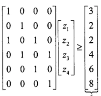
Any set of columns which 'covers' all bays with non-zero work-loads will suffice. Figure 2-1 shows columns of the initial basis used for a ship with 2 bays, 2 QCs allocated

(33)

1 0 0 0 3 0 1 0 0 z 2 1 0 1 0 z2 2 0 1 0 1 z3 4 0 0 1 0 [z4_ 6 0 0 0 1 8 fi

Figure 2-1. Example of an initial feasible column pool for a ship with parameters H= 6, C= 2 and r= 1 and clearance of 1. Note the feasibility of the columns in terms of the clearance constraints, i.e. at least 1 'empty' row always separates 2 active rows.

The pseudo-code of the procedure for generating the initial column pool is as follows:

set craneposition = 1

set numCols = -1

set config[numCols,1..H] = 0

repeat

numCols = numCols + 1

Increase size of config by 1 column Re-set rows of new column to '0'

fork= 1..C-1 do

config[numCols,craneposition+k(r+1)] = 1 end for

if craneposition + k (r + 1) = H then

break out of repeat loop end if

end repeat

config is an open array which can be dynamically re-sized at runtime. It stores the

'0-1' set-covering matrix of the RMP which has numCols number of columns. The index

craneposition marks the bay position of the first QC in the current column, while the

expression craneposition + k (r + 1) indicates the bay position of the last QC.

(34)

repeat

Solve the RMP model

if RMP is feasible then

bc = Basis information from RMP

dual[j] = Dual variable associated with rowj of set-covering constraint in RMP Import dual[j] into PP

Solve PP model

if objective value of PP < 10-5 then

xU] = Feasible QC position 'pattern' with minimum reduced cost

numCol = numCols + 1

Increase size of config by 1 column

configlnumColj] = xU]

Reset RMP model.

Set initial basis of RMP with bc Import new column pool, config else

break out of repeat loop

end if else

break out of repeat loop end if

end repeat

A simplex-based algorithm is used to solve the RMP LP. To reduce the computational

work of repeatedly solving the RMP, the basis from the optimal set of columns from previous iterations of the RMP is used as the initial basis for solving the RMP in the next

iteration. The basis information is stored as bc in the pseudo-code.

Restricted Master Problem (RMP)

The purpose of the RMP is to (1) provide dual variables for the PP, and to (2) determine if the current set of QC position-assignment 'patterns' provide an optimal LP

(35)

(RMP): Minimize z, (2.22) jElI Subject to I z, f4, Vj (2.23) iel jEi z 0, Vi (2.24)

z,, U, Vi' e {P I Ceiling constraints} (2.25)

z < L, Vi' e {P I Floor constraints} (2.26)

The following is a description of notations in the RMP:

I Set of feasible QC position-assignment 'patterns' in the column pool

P Set of branching constraints in the constraint pool of this problem node

zi Number of times QC position-assignment 'pattern' i is used

fi

Work-load in bayj

The cost of including each column is '1' since the makespan is incremented by 1 when a column is used. The objective function (2.22) minimizes the total number of columns needed to meet work-load requirements. (2.23) depicts the set-covering constraints. Constraint (2.24) enforces only the non-negativity of zi, but allows columns to be used multiple times. (2.25) and (2.26) are all the branching constraints associated with the current problem node, and its effect is to discard regions of the feasible space that included fractional variables obtained in previous nodes of the search tree.

Pricing Problem (PP)

The role of PP is to provide a column that prices out profitably or to prove that none exist. The optimal dual variables associated with constraint (2.23), p, from the RMP are imported into PP.

(36)

(PP): H MinimizeX 1- L p x (2.27) j=I Subject to H Lx, =C (2.28) j=1 min{j+r,H} C

(I-x

Xj I x,, j=1.H - I (2.29a) I=j+l C

(I-

xj

)

j I x,, j= 2..H (2.29b) l=max{1,J-r} x e{0,l} (2.30)

The decision variable, xj, is '1' if a QC is positioned at bay

j

and '0' otherwise. All other notations have similar meanings as the single-ship model. The objective function (2.27) arises from the calculation of the reduced cost of a non-basic column, indexed by i, in an LP: c, - (c B-1

)A,,

_{where ci is the cost of a non-basic column i ('1' in this case),}

(c

B-' ) is equivalent to p (the optimal dual variables associated with constraint (2.23) in

the RMP), and Ai is the non-basic column vector in i represented by xj's in the PP.

Constraint (2.28) states that all QCs must be positioned at a particular bay, therefore there are a total of C 'active' rows. (2.29) enforces QC clearance constraints similar to that of the single-ship model. QC ordering constraints (such as in (2.5) and (2.6)) are not necessary since QCs will be assigned in order of their numbering (in the k index) from the top to bottom of the column.

Column Generation at every node of branch-and-bound-tree

The LP relaxation solved by the column generation technique does not necessarily produce integer solutions, and applying a standard branch-and-bound procedure to the RMP with its existing columns does not guarantee optimality. There may be columns outside the current pool which may have negative reduced cost after branching in subsequent nodes occurs. Therefore, the branch-and-bound procedure must be modified

(37)

so that the column generation procedure is used at every node of the search tree to generate a lower bound.

2.3.3 Branching and Pruning

Branching

A valid branching scheme partitions the solution space in such a way that the current fractional optimal solution of a node is excluded, integer solutions remain intact, and finiteness of the algorithm is ensured [21]. The use of standard variable branching often creates problems along a branch where a particular variable has been set to '0'; in future iterations of PP, columns that were previously excluded may be re-generated causing cycling in the branch-and-bound algorithm. However in this case it would occur infrequently because the decision variables of the RMP, z's, are not binary. The standard variable branching rules will not force the fractional column out of the basis, hence the branched variables will have a reduced cost of zero (being basic in the LP) and automatically be excluded from being inserted into future column pools (refer to Step 7 in §2.3.1).

It is common to make important branching decisions at the top of the branch-and-bound tree. Because all columns have equal cost, in deciding on which fractional column-variable in the LP solution to branch on for every node in the tree, it suffices to select the first fractional column found.

Pruning

Since the costs of all the columns are integral, it is possible to discard nodes which have optimal LP values that are greater than an integer away from the upper bound, i.e.

Y > Yb,,t -1 instead of yk > Ybe, . This allows us to more easily disregard previously

partitioned regions of feasible space in searching for the optimal solution, thus significantly speeding up the branch-and-bound procedure.

(38)

The output of a successful run of the branch-and-price algorithm is Zbes,, the number

of times each feasible QC position-assignment 'pattern' is used. From Zbes,, we can use

RMP column pool data to form up values of x's, a decision variable of the original single-ship model, for each time period. Next, QCs are assumed to be working where they are positioned at all time periods. This is allowed through (2.8). We then arbitrarily re-set some 5's back to '0' so that the work requirement constraint (2.7) is met exactly (as opposed to being exceeded).

The following is the pseudo-code for the re-arrangement of data from Zbes, to x's:

for i = 1..numCols do set c = 1 if Zbes,' = 1 then forj= 1..H if config[numColsj]= 1 then xj,(i) = 1 c=c+ 1 end if end for end if end for

The following is the pseudo-code for the extraction of S 's from x's:

forall j, k, t do

8k(t) = Xjk(t)

end for

Initialize wastage[ 1..H] forj= 1..H do

Calculate amount that exceeded work requirement constraints for bayj Store amount in wastagelj]

for p = L..wastage[j], k = L..C do

if 31k(P)= 1 then J(p)= 0 end if

end for

(39)

2.4 Computational Results 2.4.1 Test Problems

A data set with 12 different problem instances was created. The problem instances are arranged in order of increasing ship bay numbers, each with varying work-loads, number of QCs allocated and clearance requirements. The main objective of using this data set is to validate the accuracy of the exact model and the proposed algorithms in producing QC position- and work-assignments that adhere to all the constraints. The secondary purpose is to compare the computational performance and quality of solution of the heuristic and branch-and-price methods against that of the exact model solved with CPLEX. Table 2-1 summarizes the various parameters of each problem instance, and provides the total number of constraints and decisions variables of the aggregated and 'disaggregated' forms of the exact model.

Table 2-1. Description of the first data set of test problems

Problem No. of No. of Aggregated Aggregated

No. H C r T constraints* variables* fo st N o .

No of const. No. of var.

SSl-1 10 2 1 61 8184 2501 5378 2501 SSl-2 10 3 1 61 15687 3721 9343 3721 SSI-3 10 4 1 61 25508 4941 14406 4941 SSI-4 10 5 1 61 37647 6161 20567 6161 SS1-5 10 2 3 61 8184 2501 5378 2501 SS2-1 20 3 3 106 55882 12826 33198 12826 SS2-2 20 4 4 106 90968 17066 51536 17066 SS2-3 20 3 5 106 55882 12826 33198 12826 SS3-1 30 3 8 143 114001 25883 67669 25883 SS4-1 40 2 8 198 109732 31878 0 0 SS4-2 40 3 8 198 211306 47718 0 0 SS5-1 50 3 8 249 0 0 0 0

* Disaggregated form of the single-ship model 0 Unknown - takes too long to execute model

A second data set is also created which contains problem instances with vessel sizes, work-loads and other parameters that are typically encountered in the operations of any major container terminal. The main purpose is of using this data set is to ensure that the proposed solution approaches can handle realistic industry conditions. Table 2-2 describes the parameters of this practical data set.

(40)

Table 2-2. Description of a second data set of practical test problems

Problem H C T No. of No. of

No. constraints* variables*

SSP-1 25 2 8 519 178561 52419

SSP-2 30 3 8 839 0 0

SSP-3 40 4 8 1385 0 0

* Disaggregated form of the single-ship model 0 Unknown - takes too long to execute model

2.4.2 Results and Analysis

First data set

All computational tests performed for this thesis were carried out using a Pentium-IV 1.6 GHz PC running OPL Studio in the UNIX environment. 4 different experiments were carried out on all problem instances in the first data set; the aggregated and disaggregated form of the exact model, the heuristic and branch-and-price solution approaches were run. The optimized makespan and computation time results of tests are tabulated in Table 2-3.

Table 2-3. Output and computational performance of the exact model and proposed solution approaches on first data set Exact Exact Heuristic Br-n-Pr.

Problem Exact Heuristic Br-n-Pr. runtime runtime runtime runtime (s)

No. makespan makespan makespan (s) (s) (s) / No. BnB

iterations SS1-1 31 31 31 0.8769 1.118 0.091 0.062/13 SS1-2 21 21 21 0.9829 1.251 0.083 0.111 /9 SS1-3 16 16 16 1.103 1.416 0.084 0.062/7 SS1-4 14 14 14 1.029 1.516 0.096 0.000/1 SS1-5 31 31 31 1.134 1.157 0.011 0.016/3 SS2-1 36 36 36 0.843 21.21 0.318 0.780/15 SS2-2 38 40 38 11.58 16.47 0.504 0.000/1 SS2-3 36 36 36 9.677 19.23 0.367 0.281 /4 SS3-1 56 56 56 6.542 ~ 120 1.047 0.000/1 SS4-1 99 99 99 25.89 0 1.838 2.706/9 SS4-2 66 70 66 368.7 0 1.826 18.84/43 SS5-1 0 86 83 0 0 2.998 102.3 / 99

0 Unknown - takes too long to execute model

CPLEX is able to solve the exact model within a reasonable time for problem instances up to 40 bays which has over 200,000 constraints and 50,000 decision variables. In contrast, for the aggregated form of the exact model, a solution was obtained in reasonable time only for problem instances of up to 30 bays. This validates the 'LP-tightness' of the strengthened model. Tests with the heuristic approach show that computational time does not exceed 3 seconds for all problem instances, a drastic